Approach to failure in porous granular materials under compression

Abstract

We investigate the approach to catastrophic failure in a model porous granular material undergoing uniaxial compression. A discrete element computational model is used to simulate both the micro-structure of the material and the complex dynamics and feedbacks involved in local fracturing and the production of crackling noise. Under strain-controlled loading micro-cracks initially nucleate in an uncorrelated way all over the sample. As loading proceeds the damage localizes into a narrow damage band inclined at 30-45 degrees to the load direction. Inside the damage band the material is crushed into a poorly-sorted mixture of mainly fine powder hosting some larger fragments. The mass probability density distribution of particles in the damage zone is a power law of exponent 2.1, similar to a value of 1.87 inferred from observations of the length distribution of wear products (gouge) in natural and laboratory faults. Dynamic bursts of radiated energy, analogous to acoustic emissions observed in laboratory experiments on porous sedimentary rocks, are identified as correlated trails or cascades of local ruptures that emerge from the stress redistribution process. As the system approaches macroscopic failure consecutive bursts become progressively more correlated. Their size distribution is also a power law, with an equivalent Gutenberg-Richter ‘b-value’ of 1.22 averaged over the whole test, ranging from 3 down to 0.5 at the time of failure, all similar to those observed in laboratory tests on granular sandstone samples. The formation of the damage band itself is marked by a decrease in the average distance between consecutive bursts and an emergent power law correlation integral of event locations with a correlation dimension of 2.55, also similar to those observed in the laboratory (between 2.75 and 2.25).

I Introduction

The compressive failure of porous sedimentary rocks is important in a range of applications in geophysics and engineering. They are used as building materials, and their failure mechanisms control the nature and timing of natural or induced hazards such as landslides and earthquakes in such materials sammonds_role_1992 ; ojala_2004 ; Heap201171 ; main_fault_2000 ; ROG:ROG1468 . In these and other cohesive granular materials failure occurs by the intermittent nucleation, propagation and coalescence of micro-cracks that generate acoustic emissions, one of the main sources of information about the microscopic dynamics of such failure processes lockner_nature_1991 ; lockner_1993 ; sammonds_role_1992 . Laboratory experiments have revealed that both the spatial structure of damage and the statistical and dynamical features of the time series of the corresponding acoustic events undergo a complex evolution when approaching macroscopic failure sammonds_role_1992 ; ROG:ROG1468 ; schorlemmer_variations_2005 . Quantitative understanding of this evolution process is indispensible to design forecasting strategies for imminent catastrophic failure ROG:ROG1468 . Triaxial loading experiments on Earth materials, well representing field conditions, showed that the beginning of the loading process is dominated by random nucleation of micro-cracks. However, in the vicinity of failure correlations dominate, i.e. damage was found to localize in narrow bands which gradually broaden sammonds_role_1992 ; ojala_2004 ; Heap201171 ; main_fault_2000 ; ROG:ROG1468 . The integrated statistics of the energy of acoustic emissions, accumulating all the events up to failure, is characterized by a power-law distribution $p(E)\sim E^{-B-1}$ where the exponent $B$ shows some degree of robustness with respect to material properties main_fault_2000 ; ROG:ROG1468 . However, in narrow time/strain windows a systematic decrease of the exponent $B$ was observed as failure is approached sammonds_role_1992 . These temporal changes have been suggested as possible diagnostic signatures of imminent catastrophic failure ROG:ROG1468 ; amitrano_2012_epjst .

The statistics of breaking bursts are usually investigated in the framework of stochastic lattice models, which are based on regular lattices of springs alava_statistical_2006 , beams timar_crackling_2011 , fibers pradhan_failure_2010 , or fuses alava_statistical_2006 ; alava_role_2008 . They have the advantage of allowing for a straightforward identification of breaking avalanches. However, they imply strong simplifications of the micro-structure of materials and on the dynamics of local breakings. Furthermore, they are typically capable of handling only tensile loading conditions. Stochastic lattice models have all reproduced the integrated power law statistics of burst size and revealed interesting effects of the amount of disorder alava_statistical_2006 ; alava_role_2008 ; hidalgo_universality_2008 ; PhysRevE.87.042816 ; hidalgo_avalanche_2009-1 , friction girard_failure_2010 ; amitrano_2012_epjst , and range of load redistribution on the value of the exponent PhysRevE.87.042816 ; raischel_local_2006 . As an alternative, the discrete element modeling (DEM) approach provides a more realistic treatment especially for cohesive granular materials which are inherently discrete cundall_discrete_1979 ; kun_study_1996 ; daddetta_application_2002 ; potyondy_bonded-particle_2004 ; hentz_discrete_2004 ; ergenzinger_discrete_2010 . In the framework of DEM both the micro-structure of the material and the dynamics of fracture can be better captured. Hence, it has successfully reproduced the spatial structure of damage under several loading conditions cundall_discrete_1979 ; kun_study_1996 ; daddetta_application_2002 ; potyondy_bonded-particle_2004 ; hentz_discrete_2004 ; ergenzinger_discrete_2010 ; carmona_fragmentation_2008 ; timar_new_2010 .

Recently, we have introduced a method in DEMs to investigate crackling noise generated by cascades of micro-fractures similar to sources of acoustic emission in experiments ourpaperinprl . Crackling bursts are identified as correlated trails of breaking particle contacts which made it possible to decompose the process of damage accumulation into a time series of bursts. By simulating uniaxial compression of cylindrical samples of sedimentary rocks we have shown that our DEM reproduces all qualitative features of the integrated statistics of the time series of acoustic events ourpaperinprl . Here we apply our model to investigate how the system approaches macroscopic failure by analyzing both the spatial structure of damage and the variation of the power law statistics of burst sizes in the approach to failure. A connection of the two is established by investigating the spatial correlation of consecutive bursts.

II Discrete element model of geomaterials

We briefly summarize the main steps of the construction of our discrete element model (DEM) which captures the essential ingredients of both the heterogeneous micro-structure of sedimentary rocks and the dynamics of the breaking process. The model has been used in Ref. ourpaperinprl to investigate the integrated statistics of crackling avalanches, i.e. the average properties in periods both up to and beyond the peak stress, respectively. Here we will examine the temporal evolution of the microstructural and mechanical properties in the approach to failure in more detail.

II.1 Heterogeneous micro-structure

In order to represent the structure of sedimentary rocks in a discrete element framework we sedimented spherical shaped particles in a cylindrical container of diameter $D_{0}$ and height $H_{0}$. During the sedimentation process particles fall one-by-one at random lateral position on the top of the growing particle layer and dissipate their kinetic energy by colliding with other particles and also with the wall of the container. The radius of particles $R$ is randomly generated according to a probability density $p(R)$. Figure 1$(a)$ illustrates the procedure of sample generation where the color code represents the particle size. The origin of the coordinate system is in the middle of the bottom plate of the cylinder and the $z$ axis is aligned with the symmetry axis.

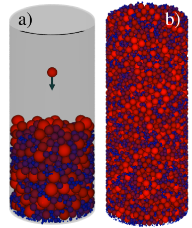
Figure 1: (Color online) $(a)$ Preparation of the sample by sedimenting spherical particles with radius $R$ sampled from a probability distribution $p(R)$. The color code corresponds to the radius of the particles such that the smallest particles are dark blue while the biggest ones have light red color. $(b)$ A complete cylindrical sample of $20000$ particles used in the simulations of the fracture process.

Molecular dynamics simulations were carried in order to generate the ballistic motion of particles of mass $m_{i}$ ($i=1,\ldots,N$) under the action of the gravitational force $\vec{F}_{i}^{g}=m_{i}\vec{g}$, where $\vec{g}$ is the gravitational acceleration. The particles fall with zero initial speed and find their equilibrium position in the random packing through a sequence of collisions. In the simulation we apply a soft particle contact model, i.e. particles overlap when they are pressed against each other which then gives rise to a repulsive force between them. Two particles $i$ and $j$ with radii $R_{i}$, $R_{j}$ and position vectors $\vec{r}_{i}$, $\vec{r}_{j}$ are in contact during their motion when the overlap distance $\xi=R_{i}+R_{j}-r_{ij}$ is positive. Here $r_{ij}$ denotes the distance of the particles $r_{ij}=|\vec{r}_{ij}|$ with $\vec{r}_{ij}=\vec{r}_{i}-\vec{r}_{j}$ pointing from particle $j$ to $i$. The interaction of the particles is described by the Hertz contact law including also viscoelastic dissipation poschel_grandyn_2005 : the contact force $\vec{F}^{c}_{ij}$ exerted by particle $j$ on $i$ is expressed in terms of the overlap distance $\xi$ as

$$\vec{F}^{c}_{ij}=-k^{p}_{ij}(\xi^{3/2}+A\sqrt{\xi}\dot{\xi})\vec{n}_{ij}.$$ (1)

The contact stiffness $k^{p}_{ij}$ depends on the material and geometrical properties of particles as $k^{p}_{ij}=2E_{p}\sqrt{R_{eff}}/3(1-\nu_{p}^{2})$, where $1/R_{eff}=1/R_{i}+1/R_{j}$, furthermore, $E_{p}$ and $\nu_{p}$ denote the Young modulus and Poisson ratio of particles’ material. The unit vector $\vec{n}_{ij}=\vec{r}_{ij}/|\vec{r}_{ij}|$ characterizes the orientation of the contact. In the force law Eq. (1) dissipation of the kinetic energy is ensured by the rate $\dot{\xi}$ dependent term, where the parameter $A$ captures the viscoelastic properties of the material. For simplicity, during the sedimentation process no tangential component of the contact force was considered. In order to generate samples with the required overall geometrical shape, bouncing particles interact with the container wall, as well. The force exerted by the wall on particle $i$ has the form

$$\vec{F}^{w}_{i}=-k^{w}_{i}(R_{i}+|\vec{r}_{i}^{r}|-D_{0}/2)\vec{r}_{i}^{r}/|\vec{r}_{i}^{r}|,$$ (2)

where $\vec{r}_{i}^{r}$ denotes the radial component of the position vector $\vec{r}_{i}$ so that $\vec{F}^{w}_{i}$ points towards the symmetry axis of the cylinder. The time evolution of sedimentation was generated by numerically solving the equation of motion of single particles

$$m_{i}\ddot{\vec{r}}_{i} = \sum_{j}\vec{F}_{ij}^{c}+\vec{F}^{w}_{i}+\vec{F}^{g}_{i},$$ (3)

where the sum over $j$ in the first term of the right hand side runs over all contacts of particle $i$. Eq. (3) is solved for each particle independently assuming all other particle positions to be frozen. In the simulations a 3$rd$ order Predictor-Corrector scheme was used for the numerical solution of Eq. (3) which ensures stability and high precision allen_computer_1984 .

The single-particle sedimentation technique has several advantages for the preparation of random particle packings: the bouncing particle can solely interact with the top layer in the container, hence, those particles which are located inside the sediment can be considered fixed, and hence, they are not considered in contact searching. Since these particle positions are not updated the simulation time linearly scales with the particle number. After the energy of the sedimenting particle droped below a small threshold value the motion of the particle was stopped. In such a configuration the particle has typically small overlaps with the surrounding ones due to the action of gravity. In order to ensure a stress free initial packing we slightly displaced the sedimented particle along the direction of the sum of contact forces until all overlaps were removed without changing the radius of the particle. The efficiency of the sedimentation techniques made it possible to generate packings of $10^{6}$ particles with about 6 hours CPU time on a single core of an Intel Xeon (6 cores) processor. The disadvantage of the technique is that the size distribution of particles $p(R)$ cannot be arbitrarily broad. Very large particles may prevent sedimenting particles to fill holes around them which may create an unphysical void structure. In the opposite limit, very small particles have a high chance to bounce inside the holes between the larger ones sedimenting to the bottom of the container. This way small particles would accumulate at the bottom, while the very large ones would stay at the top of the packing creating an unphysical micro-structure.

The radius of particles $R$ was sampled from a log-normal distribution

$$p(R)\sim\exp{\left[-\frac{(\ln R-\ln\overline{R})^{2}}{2\sigma_{R}^{2}}\right]},$$ (4)

which gives a reasonable description of the statistics of particle sizes for various types of earth materials in the range of large particles (see e.g. the particle mass distribution prior to faulting in Figure 7 of Ref. Mair200025 ). To avoid size segregation of particles during sedimentation we set the range of radius $R_{min}\leq R\leq R_{max}$ such that the ratio $R_{max}/R_{min}=20$ is fixed. Then $\overline{R}$ is chosen as $\overline{R}=5R_{min}$ to have the maximum of $p(R)$ nearly in the middle of the $[\log R_{min},\log R_{max}]$ interval. In the model the smallest particle radius $R_{min}$ is used as characteristic length scale in terms of which all other lengths are expressed. The diameter $D_{0}$ and height $H_{0}$ of the cylinder were chosen to be $D_{0}=438.57R_{min}$ and $H_{0}=1008.71R_{min}$, which yields an aspect ratio $H_{0}/D_{0}\approx 2.3$ as in the experiments of Ref. Mair200025 . With this geometrical setup the number of particles used in the simulations fluctuates in a narrow interval around 20000. The final cylindrical sample with random heterogeneous micro-structure is illustrated in Fig. 1$(b)$.

Figure 2 presents the results of the analysis of the packing structure of the sample. In Fig. 2$(a)$ the size distribution of particles obtained numerically follows perfectly the analytic log-normal form. In order to test the homogeneity of the packing we determined the average particle radius $\left<R\right>$ as a function of the $z$ coordinate measured from the bottom of the container.

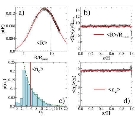
Figure 2: (Color online) Analysis of the structure of the sediment. $(a)$ The probability distribution of the particle radius in the cylindrical sample. The numerically measured distribution (symbols) has a very good agreement with the analytic curve (continuous line). $(b)$ The average radius $\left<R\right>$ of particles as a function of height $z$ inside the cylinder. The value of $\left<R\right>$ is nearly constant and it is equal to the sample average. $(c)$ Probability distribution of the contact number $n_{c}$ of particles. For $n_{c}\geq 3$ the distribution can be well described by an exponential form (green dashed line). $(d)$ The average contact number $\left<n_{c}\right>$ proved to be independent of the height along the cylinder axis.

Fig. 2$(b)$ shows that the average size is constant $\left<R\right>/R_{min}\approx 8.9$ along the cylinder axis and it is equal to the value obtained by averaging over the complete sample. Another important characteristic of the micro-structure is the number of contacts $n_{c}$ of the particles. Fig. 2$(c)$ demonstrates that the histogram of contact numbers $p(n_{c})$ can be well described by an exponential form for $n_{c}\geq 3$. A small fraction of zero contacts occurs due to some very fine particles $R\approx R_{min}$ which sediment to the bottom of the container and do not touch any other particles. Contact numbers $n_{c}=1,2,3$ typically occur along the surface of the sample while bulk particles are characterized by higher values of $n_{c}$. The exponential form of $p(n_{c})$ and the value of the average contact number $\left<n_{c}\right>\approx 5.8$ are in a reasonable agreement with measurements on Earth materials Mair200025 ; turcotte_fractals_1997 . Fig. 2$(d)$ shows that the average contact number $\left<n_{c}\right>$ does not depend on the position $z$ along the axis of the cylinder and is equal to the sample average of contact numbers. The good quality of the tests in Fig. 2$(b)$ and $(d)$ implies a high degree of homogeneity of the sample with a uniformly-random heterogeneous micro-structure.

II.2 Cohesive granular material with breakable contacts

In order to capture the cohesive interaction between the particles, first we carry out a Delaunay tetrahedrization with the position of particles in three-dimensions. Cementation between grains is represented such that the particles are coupled by beam elements along the edges of tetrahedrons. Physical properties of the beams are determined by the underlying random micro-structure of the particle packing: the equilibrium length $l_{ij}^{0}$ of the beam between particles $i$ and $j$ is the distance of the particle centers in the initial configuration $l_{ij}^{0}=|\vec{r}_{i}^{0}-\vec{r}_{j}^{0}|$, while the beam cross-section $S_{ij}$ is determined by the particle radii as $1/S_{ij}=1/(R_{i}^{2}\pi)+1/(R_{j}^{2}\pi)$. It follows that the heterogeneous micro-structure of the particle packing gives rise to randomness of the beam geometry which then shows up in the values of the physical quantities, e.g. stiffness and moduli of beams, as well.

The beam dynamics we implemented is based on Euler-Bernoulli beams as described in Refs. poschel_grandyn_2005 ; carmona_fragmentation_2008 ; PhysRevE.86.016113 as the three-dimensional generalization of the approach of Refs. kun_study_1996 ; daddetta_application_2002 . For the quantitative characterization of the deformation of beams a local coordinate system is attached to each particle at the beam ends. As the particles undergo translational and rotational motion the beams suffer elongation, compression, shear, and torsion resulting in forces and torques. The axial force $\vec{F}^{b}_{ij}$ exerted by the beam connecting particles $i$ and $j$ on particle $i$ is expressed in terms of the beam elongation $\Delta l_{ij}=r_{ij}-l_{ij}^{0}$ in the form

$$\vec{F}^{b}_{ij}=-k^{b}_{ij}\Delta l_{ij}\vec{n}_{ij}.$$ (5)

The beam stiffness $k^{b}_{ij}$ depends on the Young modulus $E_{b}$ and on the geometrical features of the beam as $k^{b}_{ij}=E_{b}S_{ij}/l_{ij}^{0}$. A dissipative component of the force is also added to Eq. (5) similar to the one used in the packing generation. The flexural forces and torques can be determined by tracing the change of the orientation of beam ends with respect to the body fixed coordinate system $\vec{e}_{x}^{b},\vec{e}_{y}^{b},\vec{e}_{z}^{b}$ of the particles, where $\vec{e}_{x}^{b}$ is aligned with the beam orientation poschel_grandyn_2005 . In a simple case when both beam ends rotated around the $\vec{e}^{b}_{z}$ axis of the body fixed system by angles $\Theta_{i}^{z}$ and $\Theta_{j}^{z}$ the resulting force and torque acting on particle $i$ can be cast into the form poschel_grandyn_2005

$$\vec{Q}^{z,b}_{i} = 3E_{b}I_{ij}\frac{\Theta_{i}^{z}+\Theta_{j}^{z}}{(l_{ij}^{0})^{2}}\vec{e}_{y}^{b},$$ (6)

$$\vec{M}^{z,b}_{i} = E_{b}I_{ij}\frac{\Theta_{i}^{z}+\Theta_{j}^{z}}{l_{ij}^{0}}\vec{e}_{z}^{b}+\left(\vec{Q}^{z,b}_{i}\times|\vec{r}_{ij}|\vec{e}_{x}^{b}\right),$$ (7)

where $I_{ij}$ denotes the beam’s moment of inertia. Torsion arises due to the relative rotation around the $\vec{e}_{x}^{b}$ axis which gives rise to the moment

$$\vec{M}^{x,b}_{i}=G_{ij}I^{t}_{ij}\frac{\Theta_{i}^{x}-\Theta_{j}^{x}}{l_{ij}^{0}}\vec{e}_{x}^{b}.$$ (8)

Here $G_{ij}$ is the shear modulus of the beam, while $I^{t}_{ij}$ denotes the torsional moment of inertia calculated with respect to the beam axis. Beam forces and torques must be transformed to the global coordinate system of the particle packing where the equation of motion is solved numerically for the translational and rotation degrees of freedom allen_computer_1984 . The same 3rd order Predictor-Corrector solver is used for the simulations as for the generation of the initial particle packing including quoternions for the representation of rotations allen_computer_1984 .

In order to capture crack formation in the model, beams break when they get overstressed during the evolution of the system. The breaking of a beam is mainly caused by stretching and bending, hence, we implemented a von-Mises type breaking criterion widely used in the literature kun_study_1996 ; daddetta_application_2002 ; carmona_fragmentation_2008

$$\left(\frac{\varepsilon_{ij}}{\varepsilon_{th}}\right)^{2}+\frac{max(|\Theta_{i}|,|\Theta_{j}|)}{\Theta_{th}}>1.$$ (9)

Here the axial strain $\varepsilon_{ij}$ of the beam is determined as $\varepsilon_{ij}=\Delta l_{ij}/l_{ij}^{0}$, while $\Theta_{i}$ and $\Theta_{j}$ are the generalized bending angles of the two beam ends. The first and second terms of Eq. (9) represent the contributions of stretching and bending deformations, respectively. The value of the breaking thresholds $\varepsilon_{th}$ and $\Theta_{th}$ control the relative importance of the two breaking modes such that increasing a breaking threshold decreases the contribution of the corresponding breaking mode. In the beam dynamics shear and bending are coupled so that the bending breaking mode in Eq. (9) mainly captures the shearing of the particle contacts. In the model there is only structural disorder present, i.e. the breaking thresholds $\varepsilon_{th}$ and $\Theta_{th}$ are set to the same constant values for all the beams: $\varepsilon_{th}=0.003$ and $\Theta_{th}=2^{\rm o}$. The breaking criterion Eq. (9) is evaluated in each iteration step for elongated beams and those ones which fulfill the condition are removed from the simulations. As a result of subsequent beam breaking cracks form in the sample.

Those particles which are not connected by beams, either because they have never been connected or their beam has broken, interact via Hertz contacts as described in section IIA for the packing generation poschel_grandyn_2005 . At this stage of modelling, particles themselves do not fragment, and only the connecting beams can be broken. For the material parameters of beams and particles such as Young modulus, Poisson ratio, and damping constants the same values are used as in Refs. carmona_fragmentation_2008 ; PhysRevE.86.016113 .

III Strain controlled uniaxial loading

We carried out computer simulations of the breaking process of cylindrical specimens of sedimentary rocks under uniaxial loading conditions. Strain controlled loading was performed in such a way that the top two particle layers on the top and bottom of the sample (a thickness of $2R_{max}$ each) were clamped rigidly to each other. Such clamping simulates strong coupling between the platen attached to the loading piston in a real experiment and the rock sample. Alternatively a low friction ’shim’ is sometimes used between the two as an alternate protocol to allow lateral movement of the upper and lower layer of the sample. The clamping has the effect of promoting a shear band to develop between two otherwise largely intact fragments, rather than producing a vertical tensile crack or a pervasively shattered sample. The bottom layer was fixed while the one on the top was moving downward at a constant speed $v_{0}$ which yields a constant strain rate $\dot{\varepsilon}$. The value of $\dot{\varepsilon}$ was set as $\dot{\varepsilon}\Delta t=1.8\cdot 10^{-7}$, where $\Delta t$ is the time step used to integrate the equation of motion. This is a very common laboratory experimental protocol, where the constant velocity is known as the piston stroke rate. The loading condition is illustrated by the inset of Fig. 3. The side wall of the cylinder is completely free, no confining pressure was applied.

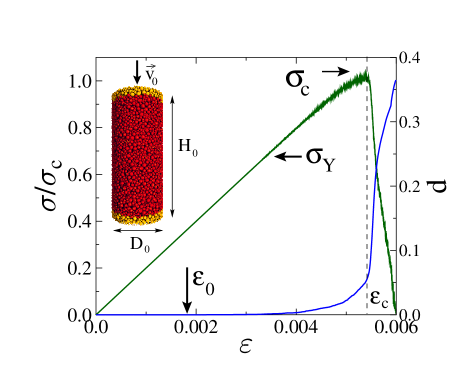
Figure 3: (Color online) Constitutive behavior $\sigma(\varepsilon)$ of a single sample (left axis) together with the accumulated damage $d(\varepsilon)$ (right axis). The large arrow and the vertical dashed line indicate the onset of beam breaking $\varepsilon_{0}$ and the position of the maximum stress $\sigma_{c}$ of the constitutive curve at $\varepsilon_{c}$, respectively. The constitutive curve is presented in a dimensionless form by rescaling the stress with its critical value $\sigma_{c}$. The inset illustrates the loading condition such that the bottom and top layers, highlighted by gold (light) color, are clamped. The top layer moves downward with velocity $v_{0}$ while the bottom is fixed. The visual yield point (discernible departure from linearity) is marked as $\sigma_{Y}$.

The macroscopic axial strain $\varepsilon$ of the sample was obtained as

$$\varepsilon=\Delta H/H_{0},$$ (10)

where $\Delta H$ is the displacement of the top layer (see inset of Fig. 3). In order to characterize the mechanical response of the sample we measure the force $\vec{F}^{t}$ acting on the top layer, which is needed to maintain the deformation $\varepsilon$. The axial stress $\sigma$ is determined as

$$\sigma=F^{t}_{y}/(\pi D_{0}^{2}/4),$$ (11)

where $F^{t}_{y}$ denotes the vertical component of the total force $\vec{F}^{t}$. The constitutive curve $\sigma(\varepsilon)$ of the system is presented in Fig. 3 together with the cumulative damage $d(\varepsilon)$ defined as the fraction of broken beams.

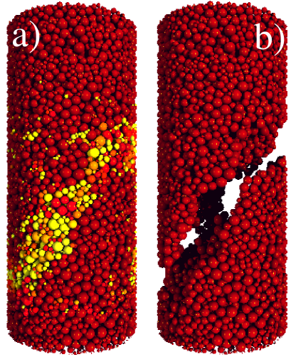
Figure 4: (Color online) $(a)$ Re-assembled sample in the final state of the simulation. Particles are placed back to their original location in the cylinder and they are colored according to the size of the fragment they originally belonged to. Hence, the two big residues are dark red, single particles have yellow color, while other colors indicate fragment sizes between the two limits. The damage band can clearly be observed on the surface of the cylindrical sample. $(b)$ To have a better view on the damage band, we only present the two big pieces of the specimen without the small sized fragments. The width and the orientation of the damage band can be better inferred from this representation.

The system has a highly brittle response: for small deformations linearly elastic behavior is obtained, stronger non-linearity of $\sigma(\varepsilon)$ is only observed in the vicinity of its maximum. The position $\varepsilon_{c}$ and value $\sigma_{c}$ of the maximum stress characterize the ultimate strength of the sample. Deviations from linear elasticity in the stress-strain curve are associated with the onset of damage due to beam breaking, indicated by the large vertical arrow on Fig. 3. However, there is a large delay before the non-linearity becomes obvious. This means that the ‘yield point’ commonly identified by the onset of discernible non-linearity in the stress-strain curve ($\sigma_{Y}$ in Fig. 3), is likely to be an overestimate, and that linearity cannot be taken as diagnostic evidence of elastic behaviour. The fluctuations in stress also become more obvious and grow after $\sigma_{Y}$, as systematically-larger bursts occur in the approach to peak stress. For a real laboratory test with a finite detection threshold for acoustic emission magnitude set by the ambient noise level, this early onset of damage would not be discernible. Similarly the stress strain curves are usually much smoother in real laboratory tests, even beyond the peak stress (e.g. similar curves in sammonds_role_1992 ; ojala_2004 ; Heap201171 ; Mair200025 ). This could be due, in part at least, to other forms of silent damage not modelled here, e.g. by environmentally-assisted, quasi-static stress corrosion sabine_PhysRevE.88.032802 ; danku_PhysRevLett.111.084302 . The damage continues to increase well into the period of dynamic stress drop. The simulation stops when the force acting on the top layer drops down to zero. The average CPU time needed to complete the compression simulation of a single sample of 20000 particles is about 5 hours on a single core of an Intel Xeon (6 cores) processor.

IV Formation of a damage band

During the loading process the weakest contacts break first. Due to the structural disorder of the sample, these breaking events give rise to micro-cracks randomly scattered all over the sample. Simulations revealed that as loading proceeds, damage localizes to a narrow spatial region where gradually a high fraction of beams break and a macroscopic crack emerges spanning the entire cross section of the sample. Figure 4 presents a representative example of the final breaking scenario of the sample. To have a clear view on the localized damage, the sample is reassembled in such a way that the particles are placed back to their original position and they are colored according to the size of the fragment they belong to. By fragments here we mean both individual particles whose beams are all broken, or clusters of two or more particles still connected by at least one beam. Figure 4$(a)$ shows the complete cylindrical sample, while in Fig. 4$(b)$ only the two big intact fragments or ’residues’ are highlighted. One can clearly observe the geometrical shape of the damage band which has a well defined orientation. The damage band comprises a large number of small sized fragments, i.e. individual particles and small fragments composed of a few particles. The quantitative analysis of $740$ samples from the different model runs revealed that the angle of the deformation band with respect to the load direction falls always between $30$ and $45$ degrees. This is similar to the angle measured in real experiments, implying a coefficient of internal friction between 0 and 0.7. In nature real faults are typically aligned with an angle of 30 degrees or so to the maximum principal stress paterson_book_1978 , although much lower coefficients of internal friction can be inferred in materials such as unconsolidated water-saturated clay.

The damage band gradually evolves and its final width reaches some $5-8$ average particle diameters. The high concentration of damage implies that the majority of beams are broken inside the band, however, not all of them are. Inside the deformation band spherical particles connected by the surviving intact beams form fragments which are embedded into the background of single particles (fine powder in the model). These fragments emerge as the width of the band increases by gradually crushing the major pieces along the sheared faces. We determined the mass distribution $p(m)$ of fragments averaging over 600 simulations. In Figure 5 three regimes of the fragment mass distribution can be distinguished:

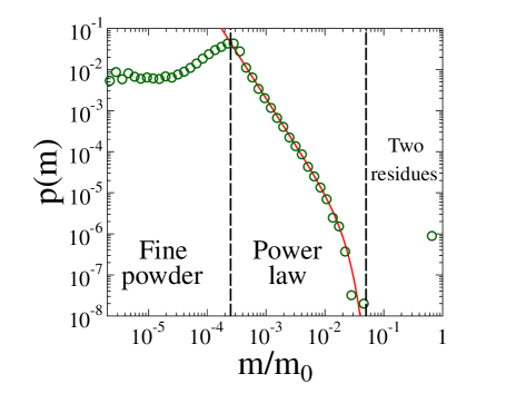
Figure 5: (Color online) Mass distribution of fragments in the final state of the simulations. Three regimes can be distinguished: the two big residues illustrated in Fig. 4$(b)$ give rise to the single peak at about a few tenths of the total sample mass $m_{0}$. A large fraction of fragments forms the fine powder which comprises single particles and very small fragments of a few particles. In the medium range the fragments have a power law distribution with a stretched exponential cutoff. The red line represents the fit obtained with Eq. (12).

The two big residues give rise to the peak at about a few tens of the total mass of the sample $m_{0}$. The majority of fragments form the fine powder on the left of the figure. These fragments comprise a single particle or a few particles up to 3-4, hence, their mass distribution is mainly determined by the original size distribution of the sedimented spherical particles. The most remarkable result is that in the intermediate range the fragments have a power law mass distribution over nearly two orders of magnitude. The numerical results were fitted by the functional form

$$p(m)\sim m^{-\tau}\exp{\left[-(m/m^{*})^{\mu}\right]},$$ (12)

where the cutoff has a stretched exponential form. A best fit in Fig. 5 was obtained with the parameter values $\tau=2.1$, $\mu=2.0$, and $m^{*}/m_{0}=0.015$. A power law distribution of fragment sizes is also typically observed in fault wear products (gouge) in natural and laboratory faults sammis_pag_1987 ; Biegel1989827 ; turcotte_factals_1986 ; steacy_automaton_1991 ; turcotte_fractals_1997 . Several mechanism-based theoretical models have been proposed where the power law size distribution is the direct consequence of the scale-invariance built into the breaking mechanism steacy_automaton_1991 ; turcotte_fractals_1997 . In our DEM the gradual compression of the specimen naturally leads to the emergence of a power law distribution in the intermediate mass range. This may imply that after the localization of damage the subsequent broadening of the deformation band by gradually crushing the surrounding material involves some degree of self similarity. This broadening of the shear band and relatively uniform geometric properties of its contents has also been observed in laboratory experiments on natural sandstones Mair200025 and has been validated independently by modeling and measurement of the evolution of fluid permeability across the band main_fault_2000 . In real laboratory and experimental faults of the frequency-length distribution for particles of fault gouge measured by a laser particle size analyser is $N(l)\sim l^{-D}$, with an exponent $D$ around $2.6$ turcotte_fractals_1997 ; sammis_pag_1987 ; Biegel1989827 ; turcotte_factals_1986 ; steacy_automaton_1991 . The probability-density distribution exponent for length is then $3.6$. For spherical particles of constant density, as here, the volume $V\sim m\sim l^{3}$ so $p(m)=p(l)dl/dm\sim m^{-(1+D)/3}m^{1/3-1}\sim m^{-\tau}$, where $\tau=1+D/3$. If $D=2.6$ then $\tau=1.87$, compared to $2.1$ in our simulations. The remaining discrepancy is likely due to the angularity (non-sphericity) of real fault gouge turcotte_fractals_1997 , when mass will not necessarily scale with the cube of linear dimension, to differences in density for the different minerals involved, and perhaps to the fact that individual particles cannot be crushed in the model.

V Crackling noise during fracture

In spite of the relatively smooth macroscopic response of the system presented in Fig. 3, at the micro-level the breaking of beams evolves in an intermittent way. The structural heterogeneity of the material has an important effect on the beginning of the breaking process which is dominated by the uncorrelated nucleation of micro-cracks. As the strain controlled loading proceeds consecutive beam breakings become correlated: the stress released by broken beams gets redistributed in the surroundings which can induce additional breakings and in turn can trigger an entire avalanche of local breaking events. These correlated trails of local beam breakings or ‘bursts’ can be considered analogous to acoustic emissions generated by the nucleating and propagating cracks in laboratory experiments lockner_1993 ; carpinteri_criticality_2009 ; sammonds_role_1992 .

In our DEM simulations the breaking criterion Eq. (9) is evaluated in each iteration step of the equation of motion of the system and those beams which fulfill the condition get broken. As loading proceeds, we record the breaking time $t_{i}^{b}$ of each beam $i=1,\ldots,N_{b}$, where $N_{b}$ is the total number of broken beams. In order to quantify the temporal correlation of local breaking events and the jerky cracking process induced by the subsequent load redistribution, we introduce a correlation time $t_{c}$: if two consecutive beam breakings occur within the correlation time $|t_{i+1}^{b}-t_{i}^{b}|<t_{c}$ they are considered to belong to the same burst. The value of $t_{c}$ was set to $t_{c}=25\Delta t$, which is approximately the time needed for the elastic waves to pass the radius of the sample $D_{0}/2$. The concept of bursts defined as correlated trails of elementary events has also been used recently to study intermittent human activity based on telecommunication data kaski_kertesz_2012 .

The size of a burst $\Delta$ is defined as the number of beams breaking in the correlated sequence. Since beams represent particle contacts, the size $\Delta$ is related to the total rupture area created by the burst. Based on the above definition further useful quantities can be introduced to characterize the bursting activity accompanying the breaking process: The time of occurrence $t$ of a burst of size $\Delta$ is the arithmetic average of the time of the first and last beam breakings in the burst

$$t=(t_{\Delta}^{b}+t_{1}^{b})/2.$$ (13)

The burst duration $T$ is the difference of the time of the first and last beam breaking in the burst

$$T=t^{b}_{\Delta}-t^{b}_{1}.$$ (14)

The elastic energy $E_{j}^{b}$ stored in the deformation of beams gets released during the breaking event. The total energy $E$ released by a burst can be determined as the sum of beam energies

$$E=\sum_{j=1}^{\Delta_{i}}E_{j}^{b}.$$ (15)

The waiting time $t_{w}$ between two consecutive bursts of size $\Delta_{i}$ and $\Delta_{i+1}$ is the difference of the time of the first beam breaking of the second burst and the time of the last breaking event of the first one

$$t_{w}=t_{1}^{b(\Delta_{i+1})}-t^{b(\Delta_{i})}_{\Delta_{i}}.$$ (16)

We have seen in the previous section that the damage has an emergent, highly non-trivial spatial structure in the sample. Consequently, the spatial positioning of bursts provides also valuable information on the evolution of the fracture process. The spatial position $\vec{r}$ of a burst can be characterized by calculating the center of mass position of broken beams

$$\vec{r}=\frac{\sum_{j=1}^{\Delta}\vec{r}_{j}^{b}}{\Delta},$$ (17)

where $\vec{r}_{j}^{b}$ is the position of beam $j$ broken in the avalanche.

Figure 6 demonstrates the size of bursts $\Delta$ as a function of strain $\varepsilon$ of their appearance together with its moving average. For comparison the constitutive curve $\sigma(\varepsilon)$ of the system is also presented.

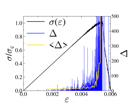
Figure 6: (Color online) Time series of burst size $\Delta$ obtained from a single model run as a function of the strain of their appearance together with the corresponding constitutive curve. The burst size $\Delta$ has strong fluctuations and on the average it increases when the maximum of $\sigma(\varepsilon)$ is approached. The moving average of $\Delta$ was calculated over 50 consecutive events.

In spite of the smooth curve of the accumulated damage $d(\varepsilon)$ in Fig. 3 the size of bursts $\Delta$ exhibits strong fluctuations while its average increases as the maximum of the constitutive curve $\sigma(\varepsilon)$ is approached. At the beginning of the breaking process only small bursts of a few breaking beams appear, however, as loading proceeds the triggering of longer avalanches becomes more probable. Strong bursting activity with complex structure of the event series emerges after the value of $\sigma$ exceeds approximately the two third of the peak stress $\sigma_{c}$. The maximum of the axis of $\Delta$ in Fig. 6 is set to 500 to be able to see the details of small sized events as well. The maximum burst size in the example is $\Delta_{max}=23417$ which was reached slightly after the peak of $\sigma(\varepsilon)$ followed by a few additional large avalanches with size $\sim 1000$ connected beam breakings. Such large sized events with long duration are the consequence of the formation of the damage band where long breaking sequences emerge due to intense fragmentation of the sample in the damage band. With the present value of the correlation time $t_{c}$ the total number of bursts we identify during the fracture process of a single sample is about 2000.

Recently, we have carried out a detailed analysis of the statistics of the size, energy, and duration of bursts, furthermore, of the waiting times between consecutive events ourpaperinprl . In this reference we considered averages integrated over the whole test before and after catastrophic failure, respectively. We showed that all quantities are power law distributed with an exponential cutoff. Careful testing of the burst identification revealed that varying the value of the correlation time $t_{c}$ only affects the cutoff. The functional form and the exponents of the distributions remained robust until $t_{c}$ falls close to the time needed for the elastic wave to pass the specimen. Single burst quantities proved to be correlated, i.e. bursts of larger size typically release a higher amount of energy and have a longer duration. These correlations are quantified by the power law dependence of the average energy and duration on the burst size ourpaperinprl . In the following we focus on the space-time variation of the crackling activity in order to understand how the slowly driven system approaches macroscopic failure.

VI Approach to failure

The beginning of the fracture process is dominated by the structural disorder of the material resulting in random nucleation of small cracks comprising only a few broken beams all over the sample. However, the subsequent stress redistribution around cracks gives rise to correlations between failure events which becomes more and more relevant as the system approaches the maximum of the constitutive curve.

VI.1 Event size statistics

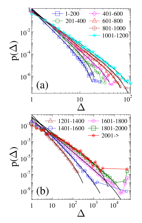
Figure 7: (Color online) Size distribution of bursts $p(\Delta)$ calculated in windows of 200 consecutive events in the time series without overlap. The thick continuous lines represent fits with Eq. (18).

Accumulating all the events up to failure, we have shown ourpaperinprl that the size distribution $p(\Delta)$ of bursts can be well described by the functional form

$$p(\Delta)\sim\Delta^{-\xi}\exp{\left[-\left(\Delta/\Delta^{*}\right)^{c}\right]}.$$ (18)

The value of the exponent $\xi$ was obtained numerically as $\xi=2.22$. In order to investigate if the exponent $\xi$ of the size distribution $p(\Delta)$ of bursts depends on when bursts were generated during the loading process the following analysis was carried out: we evaluated the size distribution $p(\Delta)$ in windows of 200 consecutive events without any overlap. Since the total number of bursts falls between 1800 and 2200 for each sample, 11 event windows could be analyzed which were averaged over 600 samples. In Figure 7 the results for the first 6 and the last 5 windows are presented separately to have a more clear view of the details. In the consecutive windows the average size of bursts increases, however, the functional form of the distribution remains nearly the same as that given by Eq. (18). Careful analysis of the data showed that rescaling the distributions by some powers of the corresponding average burst size along the horizontal and vertical axis no data collapse can be achieved. The result implies that the change of $p(\Delta)$ in Fig. 7 cannot be explained by the changing cutoff, but the exponent $\xi$ depends on the position of the event window in the time series. In Fig. 8 we present the exponent $\xi$ obtained by maximum likelihood fitting with Eq. (18) as a function of the average value of the strain where bursts occurred in a given event window.

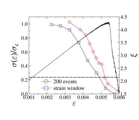
Figure 8: (Color online) The exponent $\xi$ of the burst size distribution evaluated for windows of 200 consecutive events and for equidistant bins of strain during the loading process. The dashed horizontal line represents the value of $\xi$ obtained by taking into account all the events. For clarity, we also show a representative example of the constitutive curve.

The most remarkable feature of the results is that the value of the exponent $\xi$ spans a broad interval monotonically decreasing from $\xi=4.3$ down to $\xi=1.6$ for events emerging beyond the peak of the constitutive curve. The smaller value of $\xi$ indicates that approaching the maximum of $\sigma(\varepsilon)$ the relative frequency of large events increases in the windows. This is clearly visible in Fig. 7.

The average strain of events can be slightly misleading especially for windows at the beginning of the breaking process, since here the strain of events may span a broad range with an uneven distribution. In order to avoid this problem, we also analyzed the size distribution of events in equally sized strain bins $\Delta\varepsilon=0.0005$. The functional form of the distributions on Fig. 9$(a)$ is the same as before and can be well described with a power law followed by an exponential cutoff as in Eq. (18). The value of the exponent $\xi$ obtained by fitting with Eq. (18) is also plotted in Fig. 8 at the middle points of the strain windows. In both cases the exponent spans practically the same range and have a similar dependence on the position of the measurement along the loading process. In Fig. 8 the horizontal dashed line indicates the value of the average burst size exponent $\xi=2.22$ obtained when all events are considered in the statistics. Comparing the three exponents one can conclude that the asymptotics of the distribution when all events are considered is dominated by the strongly non-linear regime of the constitutive curve before reaching the maximum.

Before comparing these results with those of laboratory tests it is necessary to discuss the way the acoustic emissions are measured, and how they scale with energy and source size. Typically the frequency-size distribution for natural earthquakes and acoustic emissions is characterised by the Gutenberg-Richter law for small and intermediate sized events: $\log(N)=a-bm$, where $a$ and $b$ are empirical constants, $N$ is an incremental frequency, and the magnitude $m$ is determined from the common logarithm of the peak amplitude of the radiated wave, corrected for attenuation with distance to the source location, so that $1$ magnitude unit is equivalent to $20dB$ in acoustics. From a simple dislocation model for the source, the relationship between magnitude and energy is $\log E=c+dm$, where $d=3/2$ if energy scales with source dimension (area) $\Delta$ as $\sim\Delta^{\nu_{E}}$, with $\nu_{E}=3/2$ (see e.g. Ref. turcotte_fractals_1997 ). We have previously shown $\nu_{E}=1.15$ (Ref. ourpaperinprl ) in our simulations rather than $3/2$. The difference is likely because the cascades of broken bonds are not necessarily planar objects, as assumed in the simple dislocation theory. From Eq. (18) the equivalent relation for the power law part is recovered in the form of the Gutenberg-Richter law if $\xi=b+1$. From this the typical value of $b$ in Figure 8 is $1.22$, ranging from $3$ or so at the start of the experiment down to $0.5$ at or near catastrophic failure. The average is very close to the typical value $b=1$ for natural earthquakes turcotte_fractals_1997 , and for the average in a typical laboratory test, such as the results of Ref. sammonds_role_1992 , where the ‘b-value’ ranges from around $1.7$ down to $0.7$. The laboratory tests have a more restricted range because they typically record only the largest events, and many smaller events which would otherwise contribute to the high value of $b$ early in the test are missing. Quantitatively our results then quite closely reproduce the monotonic decrease in $b$ observed in the ‘dry’ test on the porous sandstone sample in Ref. sammonds_role_1992 (their Figure $1(a)$), previously modelled in a more conceptual way by simplified cellular automaton models restricted to two dimensions main_fault_2000 ; Henderson1992905 . At this stage of modelling there is no coupling with a pore fluid phase, so it is not yet possible to reproduce the more complex fluctuations in $b$ associated with changes in effective stress as the pore pressure is introduced and varied in Ref. sammonds_role_1992 .

VI.2 Spatial statistics

By locating acoustic emissions and slowing down the failure process lockner_nature_1991 demonstrated that damage localization typically occurs near (sometimes a little before) the peak stress. Here a similar behavior is seen in the simulation results. In Fig. 9$(b)$ the spatial position of bursts with size $\Delta>5$ are presented in a single sample. Small events are scattered all over the sample, however, the large ones which occur in the vicinity of the peak load $\sigma_{c}$ are localized to a limited volume.

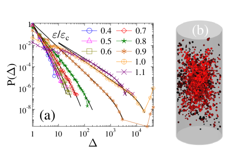
Figure 9: (Color online) $(a)$ The size distribution of bursts evaluated in equally sized strain bins $\Delta\varepsilon=0.0005$. The functional form of the curves can again be described by Eq. (18). The legend indicates the middle point of the strain bin divided by the critical strain $\varepsilon_{c}$. $(b)$ Spatial position of bursts in a single sample. Single bursts are represented by spheres with a diameter proportional to the size of the event. For clarity, only events with size $\Delta>5$ are shown. The color code illustrates the time sequence of events such that dark and light colors stand for early and late bursts, respectively.

In order to quantify how this localization develops, we calculated the average distance $\left<\Delta r_{i,i+1}\right>$ of consecutive bursts as a function of strain $\varepsilon$

$$\left<\Delta r_{i,i+1}\right>=\sqrt{\left<(\vec{r}_{i+1}-\vec{r}_{i})^{2}\right>},$$ (19)

where $\vec{r}_{i}$ and $\vec{r}_{i+1}$ are the center of mass positions of two consecutive bursts. In Figure 10$(b)$ the value of $\left<\Delta r_{i,i+1}\right>$ is normalized by the initial diameter $D_{0}$ of the cylindrical sample. At the beginning of the fracture process the average distance is practically equal to the half of the sample diameter which is the consequence of the absence of correlations. In this regime bursts are randomly scattered without any apparent correlation. The vertical dashed line marks the strain value where the average distance between burst locations starts to decrease rapidly - a clear signature of the emerging correlation. For comparison in Fig. 10$(a)$ we also present the constitutive curve together with the average size of bursts $\left<\Delta\right>$. The figure shows that in the uncorrelated regime bursts are relatively small $\Delta<10$, while the onset of the correlated burst regime is also accompanied by the sudden increase of the average burst size. The average waiting time $\left<t_{w}\right>$ monotonically decreases in Fig. 10$(b)$ with increasing strain showing the acceleration of cracking.

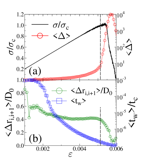
Figure 10: (Color online) $(a)$ average size of bursts $\left<\Delta\right>$ as a function of strain $\varepsilon$ together with the constitutive curve $\sigma(\varepsilon)$. $(b)$ Average waiting time between consecutive events $\left<t_{w}\right>$ and the average distance between bursts normalized by the diameter of the base circle of the cylinder as function of strain.

To obtain a more detailed description on how the spatial correlation of bursts evolves we determined the correlation integral $C(r)$ for windows of $n=200$ consecutive events similar to the b-value analysis of the size distribution of events in the previous section. The value of $C(r)$ was determined by counting the number of pairs of bursts $N(<r)$ which are separated by a distance less than $r$

$$C(r)=\frac{N(<r)}{N_{p}},$$ (20)

which was normalized by the total number of pairs $N_{p}=n(n-1)/2$ of the $n$ events of the window. In Figure 11 the distance of bursts have a lower and upper cutoff which are determined by the size of the particles and by the size of the sample, respectively. At high distances $C(r)$ converges to $1$ due to normalization. At the beginning of the fracture process $C(r)$ only saturates when $r$ spans the sample $r\approx 50\left<R\right>$ since the $n$ bursts are scattered over the complete volume. However, in the vicinity of the peak load $\sigma_{c}$, i.e. for the last 4 event windows, a power law behavior of $C(r)$ emerges

$$C(r)\sim r^{D_{2}},$$ (21)

where the correlation dimension is $D_{2}=2.55$.

This value of the correlation dimension, and the fact that the slope decreases systematically as failure approaches, compares well with the results obtained from laboratory tests on Oshima Granite GJI:GJI369 who found $D_{2}$ to be $2.75$, $2.66$ and $2.25$ for the primary, secondary and tertiary creep phases in a constant load (creep) test.

VII Conclusions

We presented a discrete element investigation of the fracture of sedimentary rocks under uniaxial compression focusing on how the system approaches macroscopic failure. The problem has a high relevance to understand the emergence of catastrophic failure in cohesive granular materials, including the failure of building materials and natural or induced events such as landslides or earthquakes occurring in sedimentary rocks, where compressive failure plays a crucial role. To generate the heterogeneous micro-structure of porous rocks, spherical particles are sedimented in a cylindrical container with a log-normal size distribution. The repulsive interaction of particles is captured by Hertz contacts, while cohesion is provided by beam elements representing the cementitious coupling of particles. Breaking of beams is induced by stretching and shearing combined in a physical breaking rule. Strain controlled uniaxial loading is realized by clamping the two opposite ends of the sample one of which was slowly moved at a constant velocity.

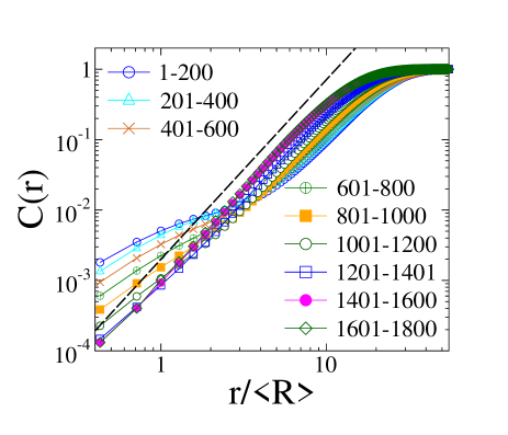
Figure 11: (Color online) Correlation integral $C(r)$ for windows of $n=200$ consecutive events. The straight line represents a power law of exponent $2.55$.

Since clamping of the sample ends promotes shear failure, damage strongly concentrated in a band. Inside the damaged band the material is mainly heavily fragmented into a fine powder of single particles or clusters of at most a few still-connected particles, however it also contains larger fragments with a power law mass distribution. The results are in a good qualitative agreement with the size distribution of fault wear products both in natural and laboratory faults turcotte_factals_1986 ; turcotte_fractals_1997 ; steacy_automaton_1991 . The power law behavior imply that the gradual cracking of the sample as the damage band broadens involves some degree of self-similarity. The value of the exponent $\tau=2.1$ is higher than the one found in DEM simulations of the impact induced dynamic breakup of heterogeneous materials in three dimensions $\tau=1.8-1.9$ carmona_fragmentation_2008 ; timar_new_2010 ; PhysRevE.86.016113 . It indicates that slow crushing gives rise to a lower frequency of large fragments since the major fraction of the body is comprised by two nearly intact residues.

Simulations revealed that the process of damage accumulation is not smooth, instead it is composed of cascades of microscopic breakings triggered by the subsequent load redistribution after local failure events. Such intermittent bursts of breakings are directly analogous to sources of acoustic emissions in real experiments. Here we focused on how the statistics of burst sizes and the correlation of the spatial location of bursts evolve as the system approaches macroscopic failure. Considering non-overlapping windows of 200 consecutive events we showed that the size of bursts is power law distributed with an exponent $\xi$ which decreases to $\xi\approx 1.6$ towards failure in a way that is quantitatively very similar to that seen in laboratory tests on sandstone samples. This so-called b-value anomaly has been observed both in laboratory experiments sammonds_role_1992 ; hatton_1993 ; ojala_2003 and in field measurements on earthquakes, however, most of the simpler modeling approaches applied to date have failed to reproduce this behavior of the avalanche statistics. For the fiber bundle model it was pointed out analytically in the mean field limit that gradually restricting the data evaluation to the close proximity of the failure point the size distribution of breaking avalanches exhibits a crossover from the exponent 5/2 to a lower value 3/2 pradhan_crossover_2005-1 . Later on computer simulations in the limit of localized load sharing yielded the same crossover behavior raischel_local_2006 . However, the nature of this crossover is different from the one responsible for the b-value anomaly: in FBMs the exponent of the avalanche size distribution is always 3/2 whenever events are considered in a narrow enough window irrespective of the stress level. An apparent crossover of $p(\Delta)$ was reported in a lattice model of the compressive failure of heterogeneous materials amitrano_rupture_2006 ; amitrano_2012_epjst . However, it was shown that rescaling the distributions with powers of the average burst size data collapse can be achieved, which clearly shows that the exponent is constant.

Our simulations revealed that the beginning of the failure process is dominated by the quenched disorder of the material so that small sized bursts randomly pop up all over the sample. In the vicinity of macroscopic failure spatial correlations emerge: the average distance of consecutive bursts sets to a rapid decrease and the correlation integral of events of non-overlapping windows develops a broad power law regime.

- (1) P. R. Sammonds, P. G. Meredith, and I. G. Main, Nature 359, 228 (1992)
- (2) I. O. Ojala, I. G. Main, and B. T. Ngwenya, Geophys. Res. Lett. 31, L24617 (2004)
- (3) M. Heap, P. Baud, P. Meredith, S. Vinciguerra, A. Bell, and I. Main, Earth and Planetary Science Letters 307, 71 (2011)
- (4) I. G. Main, O. Kwon, B. T. Ngwenya, and S. C. Elphick, Geology 28, 1131 (2000)
- (5) I. Main, Reviews of Geophysics 34, 433 (1996)
- (6) D. A. Lockner, J. D. Byerlee, V. Kuksenko, A. Ponomarev, and A. Sidorin, Nature 350, 39 (1991)
- (7) D. Lockner, Int. J. Rock Mech. Min. Sci. & Geomech. Abstr. 30, 883 (1993)
- (8) D. Schorlemmer, S. Wiemer, and M. Wyss, Nature 437, 539 (2005)
- (9) D. Amitrano, Eur. Phys. J. Special Topics 205, 199 (2012)
- (10) M. Alava, P. K. Nukala, and S. Zapperi, Adv. in Phys. 55, 349–476 (2006)
- (11) G. Timár and F. Kun, Phys. Rev. E 83, 046115 (2011)
- (12) S. Pradhan, A. Hansen, and B. K. Chakrabarti, Rev. Mod. Phys. 82, 499 (2010)
- (13) M. J. Alava, P. K. V. V. Nukala, and S. Zapperi, Phys. Rev. Lett. 100, 055502 (2008)
- (14) R. C. Hidalgo, K. Kovács, I. Pagonabarraga, and F. Kun, Europhys. Lett. 81, 54005 (2008)
- (15) K. Kovács, R. C. Hidalgo, I. Pagonabarraga, and F. Kun, Phys. Rev. E 87, 042816 (2013)
- (16) R. C. Hidalgo, F. Kun, K. Kovács, and I. Pagonabarraga, Physical Review E 80, 051108 (2009)
- (17) L. Girard, D. Amitrano, and J. Weiss, J. Stat. Mech., P01013(2010)
- (18) F. Raischel, F. Kun, and H. J. Herrmann, Phys. Rev. E 74, 035104 (2006)
- (19) P. A. Cundall and O. D. L. Strack, Géotechnique 29, 47–65 (1979)
- (20) F. Kun and H. J. Herrmann, Comp. Meth. Appl. Mech. Eng. 138, 3 (1996)
- (21) G. A. D’Addetta, F. Kun, and E. Ramm, Granular Matter 4, 77 (2002)
- (22) D. Potyondy and P. Cundall, Int. J. Rock Mech. Min. Sci. 41, 1329 (2004)
- (23) S. Hentz, F. V. Donzé, and L. Daudeville, Computers & Structures 82, 2509 (2004)
- (24) C. Ergenzinger, R. Seifried, and P. Eberhard, Granular Matter 13, 341 (2010)
- (25) H. A. Carmona, F. K. Wittel, F. Kun, and H. J. Herrmann, Phys. Rev. E 77, 051302 (2008)
- (26) G. Timár, J. Blömer, F. Kun, and H. J. Herrmann, Phys. Rev. Lett. 104, 095502 (2010)
- (27) F. Kun, I. Varga, S. Lennartz-Sassinek, and I. G. Main, submitted(2013)
- (28) T. Pöschel and T. Schwager, Computational Granular Dynamics (Springer, Berlin, 2005)
- (29) Computer Simulation of Liquids, edited by M. P. Allen and D. J. Tildesley (Oxford University Press, Oxford, 1984)
- (30) K. Mair, I. Main, and S. Elphick, J. Struct. Geol. 22, 25 (2000)
- (31) D. L. Turcotte, Fractals and chaos in geology and geophysics (Cambridge University Press, 1997)
- (32) G. Timár, F. Kun, H. A. Carmona, and H. J. Herrmann, Phys. Rev. E 86, 016113 (2012)
- (33) S. Lennartz-Sassinek, I. G. Main, Z. Danku, and F. Kun, Phys. Rev. E 88, 032802 (2013)
- (34) Z. Danku and F. Kun, Phys. Rev. Lett. 111, 084302 (2013)
- (35) M. S. Paterson and T.-F. Wong, Experimental rock deformation: the brittle field (Springer, Berlin, 1978)
- (36) C. Sammis, G. King, and R. Biegel, Pure Appl. Geophys. 125, 777 (1987)
- (37) R. L. Biegel, C. G. Sammis, and J. H. Dieterich, Journal of Structural Geology 11, 827 (1989)
- (38) D. L. Turcotte, J. of Geophys. Res. 91, 1921 (1986)
- (39) S. Steacy and C. Sammis, Nature 353, 250 (1991)
- (40) A. Carpinteri, G. Lacidogna, and S. Puzzi, Chaos, Solitons & Fractals 41, 843 (2009)
- (41) M. Karsai, K. Kaski, A.-L. Barabási, and J. Kertész, Scientific Reports 2, 397 (2012)
- (42) J. Henderson, I. Main, P. Meredith, and P. Sammonds, Journal of Structural Geology 14, 905 (1992)
- (43) T. Hirata, T. Satoh, and K. Ito, Geophysical Journal of the Royal Astronomical Society 90, 369 (1987)
- (44) C. G. Hatton, I. G. Main, and P. G. Meredith, J. Struct. Geol. 15, 1485 (1993)
- (45) I. Ojala, B. T. Ngwenya, I. G. Main, and S. C. Elphick, J. Geophys. Res. 108 (B5), 2268 (2003)
- (46) S. Pradhan, A. Hansen, and P. C. Hemmer, Phys. Rev. Lett. 95, 125501 (2005)
- (47) D. Amitrano, Int. J. Fract. 139, 369 (2006)