HATS-4b: A Dense Hot-Jupiter Transiting a Super Metal-Rich G star

Abstract

We report the discovery by the HATSouth survey of HATS-4b, an extrasolar planet transiting a V=$13.46$ mag G star. HATS-4b has a period of $P\approx 2.5167$ d, mass of $M_{p}\approx 1.32$ $M_{\rm Jup}$, radius of $R_{p}\approx 1.02$ $R_{\rm Jup}$ and density of $\rho_{p}=1.55\pm 0.16$ $\rm g\,cm^{-3}$$\approx 1.24\rho_{\rm Jup}$. The host star has a mass of $1.00$ $M_{\sun}$, a radius of $0.92$ $R_{\sun}$ and a very high metallicity $\rm[Fe/H]$$=0.43\pm 0.08$. HATS-4b is among the densest known planets with masses between 1–2 $M_{\rm J}$ and is thus likely to have a significant content of heavy elements of the order of 75 $M_{\earth}$. In this paper we present the data reduction, radial velocity measurement and stellar classification techniques adopted by the HATSouth survey for the CORALIE spectrograph. We also detail a technique to estimate simultaneously $v\sin{i}$ and macroturbulence using high resolution spectra.

1. Introduction

Planets that, from our vantage point, eclipse their host star as they orbit are termed transiting exoplanets (TEPs). Thanks to this fortuitous orientation of their orbits they allow us to measure a range of physical quantities that are not accessible for non-transiting systems. TEPs allow characterization of their atmospheres through the techniques of emission and transmission spectroscopy, the measurement of the projected angle between the stellar and orbital spins through the Rossiter-McLaughlin effect, the measurement of the ratio of planetary to stellar size $R_{p}/R_{\star}$ and, combined with radial velocities (RVs), a measurement of the true mass without ambiguities arising form the unknown inclination. Due to their being amenable to a more comprehensive physical characterization, TEPs have had a large impact on our rapidly evolving theories of planet formation and evolution.

One of the most basic quantities one can measure for a transiting planet is its bulk density. Coupled with models, the bulk density allows insights into the planetary composition, illustrated in a straightforward way by the fact that increasing the mass fraction of heavy elements increases the bulk density. The sample of confirmed transiting gas giants shows a large range in bulk densities. Part of this diversity is due to a population of planets with inflated radii, a phenomenon which is empirically found to appear above an orbit-averaged stellar irradiation level of $\langle F\rangle\sim 2\times 10^{8}$ erg s^-1 cm^-2 (Demory & Seager, 2011) and whose cause is not yet understood. The diversity in bulk density persists for planets with lower irradiation (e.g., Miller & Fortney, 2011), implying a large range in inferred core masses ($M_{\mathrm{C}}$) ranging from planets consistent with having negligible cores (e.g., HAT-P-18b; Hartman et al., 2011a) up to much denser planets with core masses substantially bigger than those for the giants in our Solar System (e.g., HD149026 with $M_{\mathrm{C}}\approx 67$  $M_{\earth}$; Sato et al., 2005). The core masses, and more generally the heavy element content of giants as compared to their host stars, are very informative in the context of models of planet formation, and the extreme values observed for some systems can prove to be a challenge.

A correlation between the metallicity of the stars and the heavy element content of their planets was reported early on by assuming a mechanism to produce the inflated radii dependent on the incident flux (Guillot et al., 2006; Burrows et al., 2007). More recently Miller & Fortney (2011) determined the heavy element masses for giant planets for a sample with lower irradiation levels in order to circumvent the uncertainties imposed by the unknown heating or contraction-stalling mechanism that operates at high irradiation. They find that giant planets around metal-rich stars have higher levels of heavy elements, with a minimum level $\sim$ 10–15 $M_{\earth}$ in heavy elements for stars with [Fe/H] $\lesssim$ 0. The scatter around this relation is high, and further understanding of the heavy element content of exoplanets necessitates more systems, particularly at extremes in stellar metallicity to probe the most extreme environments. Moreover, recent studies based on a larger sample size suggest that the correlation may not hold at all (e.g., Zhou et al., 2014a). In this work we present a system with extreme stellar metallicity discovered by the HATSouth survey: HATS-4b, a Jupiter radius planet of mass $1.32$  $M_{\rm J}$ orbiting a super metal-rich star.

The layout of the paper is as follows. In Section 2 we report the detection of the photometric signal and the follow-up spectroscopic and photometric observations of HATS-4. In Section 3 we describe the analysis of the data, beginning with the determination of the stellar parameters, continuing with a discussion of the methods used to rule out non-planetary, false positive scenarios which could mimic the photometric and spectroscopic observations, and finishing with a description of our global modeling of the photometry and RVs. Our findings are discussed in Section 4.

2. Observations

2.1. Photometric detection

Table 1 Summary of photometric observations

Facility	Date(s)	Number of Images	Cadence (s)	Filter
HS-1	2009 Dec–2011 Apr	12007	299	Sloan $r$
HS-2	2009 Sep–2010 Sep	10709	294	Sloan $r$
HS-3	2009 Dec–2011 Feb	2268	300	Sloan $r$
HS-4	2009 Sep–2010 Sep	5331	293	Sloan $r$
HS-5	2010 Jan–2011 May	2708	293	Sloan $r$
HS-6	2010 Apr–2010 Sep	98	295	Sloan $r$
FTS 2.0 m/Spectral	2012 Oct 20	107	82	Sloan $i$
Perth 0.6 m/Andor	2012 Nov 09	122	131	Sloan $r$
Swope 1.0 m/Site3	2012 Dec 30	20	154	Sloan $i$
PEST 0.3 m	2013 Jan 21	125	130	$R_{C}$

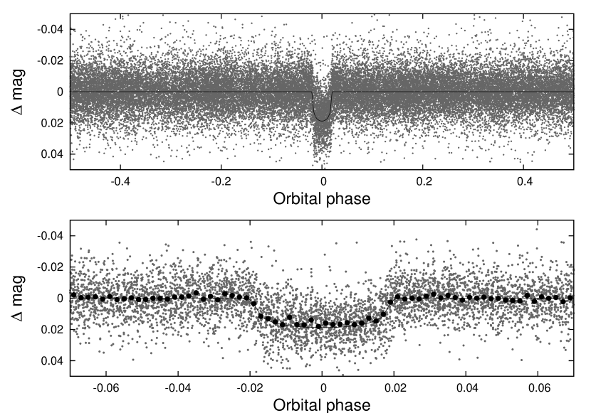
Figure 1.— Unbinned instrumental $r$-band light curve of HATS-4 folded with the period $P=2.5167286$ days resulting from the global fit described in Section 3. The solid line shows the best-fit transit model (see Section 3). In the lower panel we zoom-in on the transit; the dark filled points here show the light curve binned in phase using a bin-size of 0.002.

HATS-4b was first identified as a transiting exoplanet candidate using a light curve constructed with 33,121 photometric measurements of its host star HATS-4 (also known as 2MASS 06162689-2232487; $\alpha=06^{\mathrm{h}}16^{\mathrm{m}}26.90{\mathrm{s}}$, $\delta=-22{\arcdeg}32{\arcmin}48.8{\arcsec}$; J2000; V=$13.459\pm 0.017$mag; APASS DR5, Henden et al., 2009). The photometric measurements were obtained with the full set of six HS units of the HATSouth project, a global network of fully automated telescopes located at Las Campanas Observatory (LCO) in Chile, at the location of the High Energy Spectroscopic Survey (HESS) in Namibia, and at Siding Spring Observatory (SSO) in Australia. A detailed description of HATSouth can be found in Bakos et al. (2013). Each of the HATSouth units consist of four 0.18 m f/2.8 Takahasi astrographs, each coupled with an Apogee U16M Alta 4k$\times$4k CCD camera. Observations of 4 minutes are taken through a Sloan $r$ filter, and covered the period between Sep 2009 and May 2011. The first six entries in Table 1 summarize the HATSouth discovery observations, and the differential photometry data are presented in Table 2.3. The large number of 33,121 photometric datapoints acquired for HATS-4 is remarkable, and this was possible due to the fact this star was located at the intersection of two adjacent fields which were monitored simultaneously by each of the two units at each site. The majority of the datapoints were collected at the LCO stations HS-1 and HS-2, and very few observations were taken by the HS-6 unit in Australia as its cameras were being serviced for a large fraction of the time the relevant fields were being followed.

The photometric and candidate identification procedures adopted by HATSouth are described in Bakos et al. (2013) and Penev et al. (2013). Briefly, photometry is performed via aperture photometry, and the resulting light curves are detrended using external parameter decorrelation (EPD) and trend filtering algorithm (TFA, for a description of these procedures see the Appendix in Bakos et al., 2010 and references therein). The resulting light curves are searched for transits using the Box-fitting Least Squares (BLS) algorithm (Kovács et al., 2002). The HATS-4b discovery light curve is shown in Figure 1, folded with a period of $P=2.5167286$ days. The transit evident in this light curve triggered a follow-up process to confirm its planetary nature that we describe below.

2.2. Spectroscopy

The process of spectroscopic confirmation for HATSouth candidates is divided into steps of reconnaissance and high precision RV measurements with high resolution spectrographs. Table 2 summarizes all the follow-up spectroscopic observations which we obtained for HATS-4. The relative RVs and bisector span measurements are presented in Table 2.2. In the reconnaissance step, which utilizes spectrographs with a wide range in resolutions, we are able to exclude most stellar binary false positives. We obtained low and medium resolution reconnaissance observations of HATS-4 with the Wide Field Spectrograph WiFeS (Dopita et al., 2007) mounted on the ANU 2.3m telescope at SSO. A flux calibrated spectrum at $R\equiv\lambda/\Delta\lambda=3000$ provided an initial spectral classification for HATS-4, confirming it was a dwarf and excluding false positive scenarios that involve giants. Multiple-epoch observations at a higher resolution $R=7000$ allowed us to rule out variations in RV with amplitudes $>1$ $\rm km\,s^{-1}$ which would indicate the system is an eclipsing binary. Details of WiFeS and the data reduction and analysis procedures adopted for stellar parameter and RV measurement in the HATSouth survey have been presented in Bayliss et al. (2013).

After HATS-4b had passed the reconnaissance with WiFeS it was scheduled to be observed on higher resolution facilities capable of delivering high precision RVs. For HATS-4b, we obtained a total of 57 spectra with four such spectrographs as summarized in Table 2. We now briefly describe the observations and data reduction procedures adopted for each of these spectrographs.

Twenty-four observations were obtained with the Planet Finder Spectrograph (PFS Crane et al., 2010) mounted on the Magellan II (Clay) telescope at LCO. We obtained two I₂-free templates on the night of Dec 28 2012 UT with a slit width of 0$\farcs$3, while the remaining observations were taken through an I₂ cell and a slit width of 0$\farcs$5 on the nights of Dec 28-31 2012. A large number of exposures with PFS were taken in-transit with the aim of measuring the Rossiter-McLaughlin (R-M) effect (see § 3.2). Exposures were read out using $2\times 2$ binning on the CCD in order to increase the signal-to-noise ratio (S/N), which was typically $\approx$ 70 per resolution element for the I₂-free templates and in the range 30–90 for the spectra taken through I₂. Reduction of the PFS data was carried out using a custom pipeline and the RVs were measured using the procedures described in Butler et al. (1996).

We also observed HATS-4 with the High Dispersion Spectrograph (HDS, Noguchi et al., 2002) mounted on the Subaru telescope on the nights Sep 19-22 2012, obtaining three I₂-free templates and eight spectra taken through an I₂ cell. We used the KV370 filter with a 0$\farcs$6$\times$2″slit, resulting in a resolution $R=60,000$ and wavelength coverage 3500–6200 Å. Exposures were read out using $2\times 1$ binning on the CCD in order to increase the S/N, which was typically $\approx$ 130 per resolution element for both the I₂-free templates and the ones taken through I₂. RVs were measured using the procedure detailed in Sato et al. (2002, 2012) which are in turn based on the method of Butler et al. (1996). Bisector span measurements were measured following Bakos et al. (2007).

Finally, observations were also obtained with the FEROS spectrograph (Kaufer & Pasquini, 1998) mounted on the ESO/MPG 2.2m telescope and with the CORALIE spectrograph (Queloz et al., 2001a) mounted on the Euler 1.2m telescope in La Silla. Descriptions of the data reduction procedures for these spectrographs have been detailed in papers reporting previous HATSouth discoveries (Penev et al., 2013; Mohler-Fischer et al., 2013). The CORALIE procedures were only briefly described in Penev et al. (2013). In the Appendix we describe in more detail reduction and RV measurement procedures which we have developed and applied in the context of HATSouth follow-up for CORALIE.

HATS-4 is a metal-rich dwarf with low rotation, allowing in principle very high precision RVs to be measured, but its relative faint magnitude limits the precision that can be obtained in a single measurement, especially for the spectrographs mounted on smaller telescopes.

Table 2 Summary of spectroscopic observations

Telescope/Instrument	Date Range	Number of Observations	Resolution	Observing Mode
ANU 2.3 m/WiFeS	2012 May 8	1	3000	RECON spectral class.
ANU 2.3 m/WiFeS	2012 May 10–12	3	7000	RECON RVs
ESO/MPG 2.2 m/FEROS	2012 Aug 6	1	48000	ThAr/HPRV
Euler 1.2 m/CORALIE	2012 Aug 21–25	3	60000	ThAr/HPRV
Subaru 8.2 m/HDS	2012 Sep 19–22	8	60000	I2/HPRV
Subaru 8.2 m/HDS	2012 Sep 20	3	60000	I2-free template
Euler 1.2 m/CORALIE	2012 Nov 6–11	6	60000	ThAr/HPRV
Magellan 6.5 m/PFS	2012 Dec 28	3	127000	I2-free template
Magellan 6.5 m/PFS	2012 Dec 28–31	21	76000	I2/HPRV
ESO/MPG 2.2 m/FEROS	2012 Dec 29–31	6	48000	ThAr/HPRV
ESO/MPG 2.2 m/FEROS	2013 Jan 22–27	4	48000	ThAr/HPRV
ESO/MPG 2.2 m/FEROS	2013 Feb 24, 26	2	48000	ThAr/HPRV

Figure 2.— Top panel: High-precision RV measurements for HATS-4 from CORALIE (dark filled circles), Subaru/HDS (open triangles), FEROS (Xs) and PFS (gray-scale filled squares), together with our best-fit model. Zero phase corresponds to the time of mid-transit. The center-of-mass velocity has been subtracted. Second panel: Velocity $O\!-\!C$ residuals from the best-fit model. The error bars for each instrument have been inflated such that $\chi^{2}$ per degree of freedom is unity. Third panel: Bisector spans (BS), with the mean value subtracted. Note the different vertical scales of the panels.

Table 3 Relative radial velocities and bisector span measurements of HATS-4.

BJD	RV	$\sigma_{\rm RV}$	BS	$\sigma_{\rm BS}$	Phase	Instrument
(2 454 000$+$)	($\rm m\,s^{-1}$)	($\rm m\,s^{-1}$)	($\rm m\,s^{-1}$)
$2145.92503$	$-25.66$	$103.00$	$-80.0$	$17.0$	$0.136$	FEROS
$2160.89156$	$-172.31$	$52.00$	$86.0$	$26.0$	$0.083$	Coralie
$2161.92195$	$-116.31$	$64.00$	$-47.0$	$32.0$	$0.492$	Coralie
$2164.90865$	$244.69$	$52.00$	$2.0$	$26.0$	$0.679$	Coralie
$2190.11092$	$172.54$	$8.05$	$0.5$	$47.4$	$0.693$	HDS
$2190.12564$	$175.03$	$7.41$	$0.0$	$31.1$	$0.699$	HDS
$2191.09557\tablenotemark{c}$	$\cdots$	$\cdots$	$23.9$	$28.3$	$0.084$	HDS
$2191.11040\tablenotemark{c}$	$\cdots$	$\cdots$	$3.7$	$19.1$	$0.090$	HDS
$2191.12511\tablenotemark{c}$	$\cdots$	$\cdots$	$9.6$	$15.4$	$0.096$	HDS
$2192.08553$	$-12.54$	$7.67$	$13.7$	$49.6$	$0.477$	HDS
$2192.10026$	$-2.29$	$8.80$	$-20.6$	$63.1$	$0.483$	HDS
$2192.11498$	$-8.90$	$8.29$	$36.6$	$29.1$	$0.489$	HDS
$2193.07700$	$135.58$	$9.52$	$-35.1$	$48.0$	$0.871$	HDS
$2193.09173$	$138.86$	$7.95$	$-30.5$	$50.9$	$0.877$	HDS
$2193.10646$	$125.48$	$6.77$	$-1.8$	$16.2$	$0.883$	HDS
$2237.74591$	$111.69$	$44.00$	$-28.0$	$22.0$	$0.620$	Coralie
$2238.86723$	$-100.31$	$48.00$	$47.0$	$24.0$	$0.066$	Coralie
$2239.79009$	$-62.31$	$44.00$	$-15.0$	$22.0$	$0.432$	Coralie
$2240.85420$	$167.69$	$63.00$	$85.0$	$32.0$	$0.855$	Coralie
$2241.77140$	$-67.31$	$57.00$	$-19.0$	$29.0$	$0.220$	Coralie
$2242.79877$	$140.69$	$47.00$	$-31.0$	$24.0$	$0.628$	Coralie
$2289.66456$	$-190.08$	$2.94$	$\cdots$	$\cdots$	$0.250$	PFS
$2289.68524$	$-206.68$	$3.77$	$\cdots$	$\cdots$	$0.258$	PFS
$2290.57647$	$259.34$	$100.00$	$20.0$	$17.0$	$0.612$	FEROS
$2290.71043$	$327.34$	$120.00$	$94.0$	$20.0$	$0.665$	FEROS
$2290.81055$	$187.02$	$3.31$	$\cdots$	$\cdots$	$0.705$	PFS
$2290.83195$	$205.78$	$3.74$	$\cdots$	$\cdots$	$0.713$	PFS
$2291.53588$	$14.35$	$5.55$	$\cdots$	$\cdots$	$0.993$	PFS
$2291.54701$	$-5.57$	$6.39$	$\cdots$	$\cdots$	$0.998$	PFS
$2291.55792$	$8.57$	$5.24$	$\cdots$	$\cdots$	$0.002$	PFS
$2291.56891$	$-3.16$	$5.16$	$\cdots$	$\cdots$	$0.006$	PFS
$2291.57843$	$46.34$	$96.00$	$15.0$	$17.0$	$0.010$	FEROS
$2291.58011$	$5.48$	$4.81$	$\cdots$	$\cdots$	$0.011$	PFS
$2291.58849$	$-35.90$	$10.38$	$\cdots$	$\cdots$	$0.014$	PFS
$2291.60172$	$-17.41$	$4.37$	$\cdots$	$\cdots$	$0.019$	PFS
$2291.61378$	$-26.72$	$4.99$	$\cdots$	$\cdots$	$0.024$	PFS
$2291.62559$	$-27.07$	$4.40$	$\cdots$	$\cdots$	$0.029$	PFS
$2291.63700$	$-44.46$	$4.43$	$\cdots$	$\cdots$	$0.033$	PFS
$2291.64813$	$-39.03$	$5.12$	$\cdots$	$\cdots$	$0.038$	PFS
$2291.65109$	$20.34$	$93.00$	$48.0$	$16.0$	$0.039$	FEROS
$2291.65909$	$-52.96$	$4.28$	$\cdots$	$\cdots$	$0.042$	PFS
$2291.67013$	$-54.64$	$4.28$	$\cdots$	$\cdots$	$0.047$	PFS
$2291.68108$	$-46.23$	$5.55$	$\cdots$	$\cdots$	$0.051$	PFS
$2291.69219$	$-66.57$	$4.47$	$\cdots$	$\cdots$	$0.055$	PFS
$2292.56735$	$-57.66$	$100.00$	$-9.0$	$17.0$	$0.403$	FEROS
$2292.61509$	$-103.30$	$3.33$	$\cdots$	$\cdots$	$0.422$	PFS
$2292.63646$	$-96.78$	$3.76$	$\cdots$	$\cdots$	$0.430$	PFS
$2292.86458$	$153.34$	$121.00$	$33.0$	$20.0$	$0.521$	FEROS
$2314.72311$	$-198.66$	$62.00$	$-9.0$	$12.0$	$0.206$	FEROS
$2315.70746$	$64.34$	$66.00$	$-11.0$	$12.0$	$0.598$	FEROS
$2318.72346$	$118.34$	$61.00$	$-20.0$	$12.0$	$0.796$	FEROS
$2319.66753$	$-206.66$	$62.00$	$-23.0$	$12.0$	$0.171$	FEROS
$2347.60681$	$-194.66$	$58.00$	$-30.0$	$11.0$	$0.272$	FEROS
$2349.55979$	$-107.66$	$58.00$	$-19.0$	$11.0$	$0.048$	FEROS

[-1.5ex]

2.3. Photometric follow-up observations

High precision photometric follow-up of HATS-4, necessary to determine precise values of the orbital parameters and the planetary radius, was performed using four facilities: the Spectral camera on the 2m Faulkes Telescope South (FTS) at SSO, the SITe3 camera on the Swope 1m telescope at LCO, the 0.3 m Perth Exoplanet Survey Telescope (PEST) and the Andor camera on the Perth 0.6m telescope. We observed three partial and one full transit, the light curves are shown in Figure 3 and the differential photometry for the light curves is presented in Table 2.3.

Details of the instruments, observation strategy, reduction and photometric procedures for Spectral/FTS, SITe3/Swope and PEST can be found in Bayliss et al. (2013), Penev et al. (2013), and Zhou et al. (2014b), respectively. This is the first time we present data from the Perth 0.6 m: on 2012 November 9 we monitored the transit of HATS-4 with the Andor iKon-L CCD camera coupled to the 0.6 m Perth-Lowell Automated Telescope at Perth Observatory, Australia. We used an $r$-band filter and exposure times of 100 s. Standard bias, dark, and flat-field corrections were performed using the Perth-Lowell Automated Telescope automated reduction pipeline. Aperture photometry was performed following the methods described in Bakos et al. (2010) with modifications appropriate for this facility.

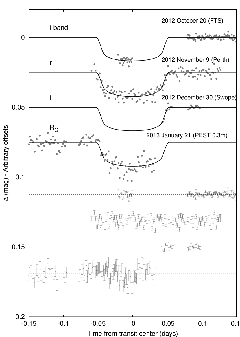
Figure 3.— Unbinned instrumental Sloan $r$- and $i$-band, and Cousins $R_{C}$ transit light curves of HATS-4. The dates and instruments used for each event are indicated. The light curves have been detrended using the EPD process. Curves after the first are shifted for clarity. Our best fit is shown by the solid lines. Residuals from the fits are displayed at the bottom, in the same order as the top curves.

Table 4Differential photometry of HATS-4

Note. — This table is available in a machine-readable form in the online journal. A portion is shown here for guidance regarding its form and content.

3. Analysis

3.1. Stellar Parameter Estimation and Global Modeling of the Data

The stellar parameters for HATS-4b were estimated using the Stellar Parameter Classification (SPC) procedure (Buchhave et al., 2012) using the I₂-free templates obtained with PFS. The initial values of the stellar parameters obtained with SPC were $T_{\rm eff\star}$$=5403\pm 50$ K, $\log{g}$$=4.46\pm 0.1$, $\rm[Fe/H]$$=0.43\pm 0.08$ and $v\sin{i}$$=1.5\pm 0.5$ $\rm km\,s^{-1}$.

Joint global modeling of the available photometry and RV data was performed following the procedure described in detail in Bakos et al. (2010). Light curves were modeled using the expressions provided in Mandel & Agol (2002) together with EPD and TFA to account for systematic variations due to external parameters and common trends of the ensemble of stars in a given set of observations. The RV data was modeled with a Keplerian orbit following the formalism of Pál (2009). The best fit parameters are first estimated via a maximization of the likelihood using a downhill simplex algorithm. This is followed by a Monte Carlo Markov Chain (MCMC) analysis to estimate the posterior distribution of the parameters.

Following Sozzetti et al. (2007) we use the values of $T_{\rm eff\star}$ and $\rm[Fe/H]$ obtained from SPC together with the stellar mean density $\rho_{\star}$ inferred from the transit to constrain mass, radius, age and luminosity of HATS-4 using the Yonsei-Yale (YY) stellar evolution models (Yi et al., 2001). In each step of the MCMC run as part of the global modeling, the current sample values for $T_{\rm eff\star}$, $\rho_{\star}$ and $\rm[Fe/H]$ are used to interpolate from the YY isochrones values for mass, radius, age and luminosity, building thus posterior distributions for them and derived quantities such as $\log{g}$. This process usually results in a more precise value of $\log{g}$ than that inferred from spectroscopy alone, and this new estimate for $\log{g}$ can be fixed in a new spectroscopic analysis to infer new values of $T_{\rm eff\star}$, $\rm[Fe/H]$ and $v\sin{i}$. The new values obtained are also used to update the limb darkening parameters (taken from Claret, 2004) which are needed to model the light curves and are dependent on stellar parameters. This process is iterated until the isochrone-revised $\log{g}$ value is consistent within $1\sigma$ with the input estimate. In the case of HATS-4 the isochrone-revised value of $\log{g}$ was consistent with the original SPC value quoted above and therefore no iterations were necessary.

The stellar parameter estimates, along with 1$\sigma$ uncertainties resulting from the process described above, are listed in Table 5. The inferred location of the star in a diagram of $a/R_{\star}$ versus $T_{\rm eff\star}$ is shown in Figure 6. Finally, the global modeling estimates of the geometric parameters relating to the light curves and the derived physical parameters for HATS-4b are listed in Table 6. We find that the planet has a mass of $M_{p}\approx 1.32$ $M_{\rm J}$, and radius of $R_{p}\approx 1.02$ $R_{\rm J}$, which results in a planet that is not inflated and has a density of $\rho_{p}=1.55\pm 0.16$ $\rm g\,cm^{-3}$. Note that we allow the eccentricity to vary in the fit so as to allow our uncertainty on this parameter to be propagated, but we find the eccentricity to be consistent with that of a circular orbit.

One of the most remarkable properties of HATS-4 is its high value of $\rm[Fe/H]$=$0.43\pm 0.08$. Of all the planet hosting stars listed in exoplanets.org as of January 2014, only four stars have $\rm[Fe/H]$$>0.43$ dex, placing HATS-4 among the 1% most metal-rich planet hosting stars. To illustrate the high $\rm[Fe/H]$ of HATS-4, we show in Figure 4 a portion of the PFS spectrum of HATS-4 with a few unsaturated metallic lines and overlay PHOENIX models (Husser et al., 2013) for values of $\rm[Fe/H]{}=0.0,0.5$ keeping the other stellar parameters fixed to those listed in Table 5. The figure clearly shows that high metal enrichment values are needed to account for the very deep lines present in the spectrum.

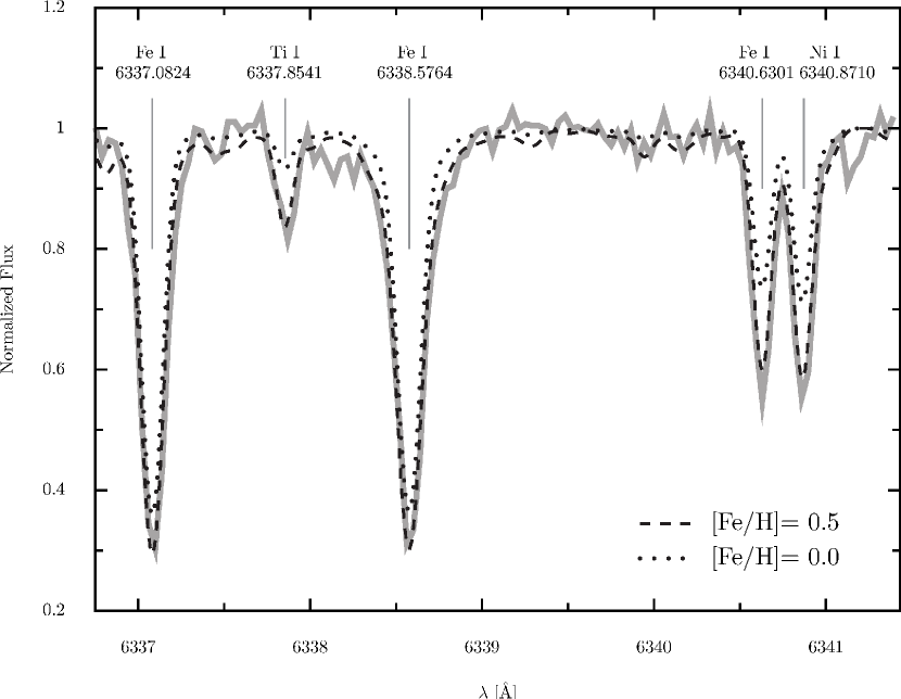
Figure 4.— Portion of an I₂-free spectrum of HATS-4 taken with PFS and containing a few metallic lines identified in the figure along with their rest-frame vacuum wavelength values. The thick gray line connects the datapoints, while the dashed and dotted lines show PHOENIX models for values of $\rm[Fe/H]$$=0.0,0.5$ as indicated, and with the rest of the stellar parameters fixed to the values listed in Table 5. It is clear that the very deep lines require a high $\rm[Fe/H]$.

3.2. Estimation of $v\sin{i}$ and Macroturbulence

An initial analysis of the FEROS spectra suggested that $v\sin{i}$ was $5\pm 2$ $\rm km\,s^{-1}$, and based on this information we scheduled observations with PFS through a well-placed transit event to measure the Rossiter-McLaughlin effect. For a slowly rotating G star like HATS-4 it is critical to distinguish between rotational broadening (parametrized by $v\sin i$) and broadening due to turbulence (parametrized by macroturbulence $\zeta$) when modeling the spectra. Here we describe our procedure for simultaneously measuring both of these parameters from the PFS data.

Both rotation and turbulence are large-scale motions on the surface of the star, with the latter being generated by circulation and convective cells that fill the surface. They result in a Doppler shift of the radiation that emerges from the photosphere producing a broadening of the spectral lines. For F and earlier type stars, the rotational velocity is the principal source of line broadening. On the other hand, for late-type stars like HATS-4, both velocity phenomena are generally of similar magnitude (Gray, 2005). For these stars getting some hold on macroturbulence is necessary because it broadens the lines in a comparable way to rotation, but the R-M effect due to microturbulence is much smaller (Albrecht et al., 2012; Boué et al., 2013). Any line broadening incorrectly attributed to rotation can thus adversely effect the inferences on the relative alignment of stellar and orbital spins.

Disentangling the value of $v\sin{i}$ from $\zeta$ using the width of the lines is a degenerate problem. At the velocity broadening expected for late-type dwarfs (few km s^-1), the line profile is usually dominated by the instrumental profile, and in addition it depends on the atmospheric parameters of the star. The macroturbulence velocity profile is very peaked while the rotational profile is much more shallow, and if one is able to observe lines at very high resolution and S/N, a Fourier analysis of single lines can separate both effects (Gray, 2005), a methodology that has been applied for bright stars. For fainter systems like HATS-4 this becomes prohibitive, but one can exploit the many lines simultaneously available in our spectra to constrain separately $v\sin{i}$ and $\zeta$.

The approach we followed is to select a large number of isolated, unblended and unsaturated metal lines based on a PHOENIX synthetic spectrum (Husser et al., 2013) with stellar parameters corresponding to those measured with SPC. Then this set of lines for the grid of synthetic models are convolved by the effects of $v\sin{i}$ and $\zeta$ for a grid of values which in our case was given by $\{0.1,0.2,0.3,\ldots,7.8,7.9,8.0\}$ km s^-1 for both quantities. The convolved models were generated following the radial-tangential anisotropic macroturbulence model which assumes that a certain fraction of the stellar material moves tangential to its surface and the rest of the material moves along the stellar radius (Gray, 2005). We assumed that both fractions are equal. To compute the convolved line profile, a numerical disk integration was performed at each wavelength including the macroturbulence Doppler shift at each point on the disk and also the shift due to the stellar rotation. We also include a linear limb darkening law in the disk integration procedure using the coefficients of Claret & Bloemen (2011), performing a linear interpolation to obtain the value at each wavelength.

Once we have the grid of convolved models, we compute the quantity $X^{2}=\sum_{k=1}^{K}\sum_{i}[m_{i}(v\sin{i},\zeta)-d_{i}]^{2}$, where $m_{i}(v\sin{i},\zeta)$ is the convolved model and $d_{i}$ is the observed spectrum. The index $k$ runs over the set of chosen lines while $i$ runs over the pixels belonging to each of the $K$ lines. The pair of $(\hat{v\sin{i}},\hat{\zeta})$ values producing the lowest value of $X^{2}$ is taken to be our estimates. Based on the fact that $\zeta$ and $v\sin{i}$ only change the shape of the spectral lines we normalize each line (both for the data and the models) by its total absorbed flux, in order to reduce the effect of systematic mismatches between data and models. Effectively, we are thus fitting for the line shape and not its strength. This normalization also minimizes the effect of errors in the measured $\log{g}$ and $\rm[Fe/H]$ because in the case of non-saturated metal lines, changes in these parameters mainly affect their strength but not their shape or width. To estimate the uncertainties on $v\sin{i}$ and $\zeta$, we applied a bootstrap over the chosen metallic lines. That is, we selected a set of lines with replacement from our list and re-run the fit obtaining a sample of bootstrap estimates $\{v\sin{i}_{J},\zeta_{J}\}_{J=1}^{B}$ where $B$ is the number of bootstrap replications. From the bootstrap sample we can estimate the parameter uncertainties by taking their dispersion.

We applied this method to the two I₂-free templates acquired with PFS (see § 2.2). We chose 145 lines in the range between 5200–6500 Å and due to the $2\times 2$ binning used in the observations we can sample each line with $\approx$ 10 pixels. To get the instrumental response we used the calibration ThAr spectra taken with the same slit we used in the observations. First we computed a global spectral profile median combining all the normalized emission lines of the ThAr spectrum. This global profile was very well fitted by a Gaussian. We then fitted Gaussians to each emission line to trace the instrumental response across our spectral range. A clear trend was identified in each echelle order whereby the spectral resolution increases from blue to red. This trend was accounted for by fitting to each order the width of the ThAr lines as a linear function of wavelength. We note that in observations of stellar objects the slit is illuminated by the seeing profile, while in a ThAr frame the slit is fully illuminated, leading in general to different profiles for emission lines in the ThAr frames and stellar objects in science observations. Given that the slit width we used is small compared to the full-width at half-maximum of the seeing profiles during our observations, using the ThAr frames to estimate the instrumental response is an adequate approximation.

Our method yielded values of $v\sin{i}$$=0.7\pm 0.5$ km s^-1 and $\zeta=1.3\pm 0.4$ km s^-1 for HATS-4. To test the sensitivity of our results on the assumed $T_{\rm eff\star}$, we repeated the procedure but with a synthetic model with values of $T_{\rm eff\star}$ $\pm 1\sigma$ from the SPC values, obtaining results fully consistent with the ones we quote. As a validation procedure we measured $v\sin{i}$ and $\zeta$ for $\tau$ Ceti following the same procedure as for HATS-4. The stellar parameters for $\tau$ Ceti were taken from Maldonado et al. (2012). We measured $v\sin{i}$$=0.5\pm 0.4$ km s^-1 and $\zeta=2.3\pm 0.1$ km s^-1. The $v\sin{i}$ value is in agreement with current studies which point towards $\tau$ Ceti having a rotation axis close to perpendicular to the sky and the value for $\zeta$ is in good agreement with the expected value for the spectral type of $\tau$ Ceti (Gray, 2005). We note that the total broadening by $v\sin{i}$ and $\zeta$ for HATS-4 is consistent with the value of $v\sin{i}$ estimated by SPC.

In Figure 5 we show the RVs during transit measured using PFS on the night of Dec 30 2012 (UT). Along with the data, we show the expected behavior of the RVs without considering the Rossiter-McLaughlin (R-M) effect, and the expected behavior assuming the system was aligned and $v\sin{i}$ had the value of 5 $\rm km\,s^{-1}$ initially estimated from the FEROS data. The R-M effect was calculated for RVs measured with an I₂ cell using the ARoME library (Boué et al., 2013). It is clear that with $v\sin{i}$$=5$ $\rm km\,s^{-1}$ the precision afforded by PFS would have allowed us to measure the relative projected angle between the stellar and orbital spins, but with the actual value of $v\sin{i}$$=0.5\pm 0.4$ $\rm km\,s^{-1}$ the R-M effect is barely noticeable and thus no constraints are possible.

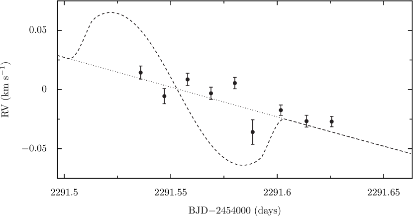
Figure 5.— Relative radial velocity (RV) measurements of HATS-4 performed during transit using PFS. The dotted line shows the unperturbed orbit using the best fit orbital parameters determined in this work without considering the RVs shown. The dashed line illustrates what the Rossiter-McLaughlin effect would look like if the system was aligned and had $v\sin{i}=5$ $\rm km\,s^{-1}$.

3.3. Excluding blend scenarios

To rule out the possibility that HATS-4 is a blended stellar eclipsing binary system we conducted a blend analysis as described in Hartman et al. (2011b). This analysis attempts to model the available light curves, photometry calibrated to an absolute scale, and spectroscopically determined stellar atmospheric parameters, using combinations of stars with parameters constrained to lie on the Girardi et al. (2000) evolutionary tracks. We find that the data are best described by a planet transiting a star. Moreover, the only non-planetary blend models that cannot be rejected with greater than $5\sigma$ confidence, based on the photometry alone, would have easily been rejected as double-lined spectroscopic binary systems, or would have exhibited very large ($\sim 1$ $\rm km\,s^{-1}$) RV and/or bisector-span variations. Such large bisector-span variations can be ruled out based on the Subaru/HDS measurements which show an RMS scatter of only $\sim 22$ $\rm m\,s^{-1}$.

Figure 6.— Model isochrones from Yi et al. (2001) for the measured metallicity of HATS-4, $\rm[Fe/H]$= $0.43$, and ages of 0.2 Gyr, and 1 to 13 Gyr in 1 Gyr increments (left to right). The adopted values of $T_{\rm eff\star}$ and $a/R_{\star}$ are shown together with their 1$\sigma$ and 2$\sigma$ confidence ellipsoids.

Table 5 Stellar parameters for HATS-4

Parameter	Value	Source
Spectroscopic properties
$T_{\rm eff\star}$ (K)	$5403\pm 50$	SPC
$\rm[Fe/H]$	$0.43\pm 0.08$	SPC
$v\sin{i}$ ($\rm km\,s^{-1}$)	$0.7\pm 0.5$	This work
$\zeta$ ($\rm km\,s^{-1}$)	$1.3\pm 0.4$	This work
Photometric properties
$V$ (mag)	$13.459\pm 0.017$	APASS
$B$ (mag)	$14.267\pm 0.020$	APASS
$J$ (mag)	$12.032\pm 0.022$	2MASS
$H$ (mag)	$11.697\pm 0.025$	2MASS
$K_{s}$ (mag)	$11.612\pm 0.021$	2MASS
Derived properties
$M_{\star}$ ($M_{\sun}$)	$1.001\pm 0.020$	YY+$a/R_{\star}$+SPC
$R_{\star}$ ($R_{\sun}$)	$0.925\pm 0.022$	YY+$a/R_{\star}$+SPC
$\log{g_{\star}}$ (cgs)	$4.51\pm 0.02$	YY+$a/R_{\star}$+SPC
$L_{\star}$ ($L_{\sun}$)	$0.65\pm 0.05$	YY+$a/R_{\star}$+SPC
$M_{V}$ (mag)	$5.38\pm 0.09$	YY+$a/R_{\star}$+SPC
$M_{K}$ (mag,ESO)	$3.54\pm 0.06$	YY+$a/R_{\star}$+SPC
Age (Gyr)	$2.1\pm 1.6$	YY+$a/R_{\star}$+SPC
Distance (pc)	$420\pm 12$	YY+$a/R_{\star}$+SPC

Table 6Orbital and planetary parameters

Parameter	Value
Light curve parameters
$P$ (days)	$2.516729\pm 0.000002$
$T_{c}$ (${\rm BJD}$)	$2455808.34095\pm 0.00036$
$T_{14}$ (days)	$0.1053\pm 0.0009$
$T_{12}=T_{34}$ (days)	$0.0112\pm 0.0006$
$a/R_{\star}$	$8.43_{-0.22}^{+0.17}$
$\zeta/R_{\star}$	$21.26\pm 0.15$
$R_{p}/R_{\star}$	$0.1132\pm 0.0029$
$b\equiv a\cos i/R_{\star}$	$0.217_{-0.093}^{+0.074}$
$i$ (deg)	$88.5\pm 0.6$
Limb-darkening coefficients
$a_{r}$ (linear term)	$0.4675$
$b_{r}$ (quadratic term)	$0.2624$
$a_{R}$	$0.4356$
$b_{R}$	$0.2718$
$a_{i}$	$0.3518$
$b_{i}$	$0.2930$
RV parameters
$K$ ($\rm m\,s^{-1}$)	$197.5\pm 3.2$
$\sqrt{e}\cos\omega$	$0.029\pm 0.039$
$\sqrt{e}\sin\omega$	$-0.097\pm 0.085$
$e\cos\omega$	$0.003\pm 0.005$
$e\sin\omega$	$-0.010_{-0.022}^{+0.010}$
$e$	$0.013\pm 0.016$
$\omega$	$275\pm 98$
CORALIE RV jitter ($\rm m\,s^{-1}$)	$29.0$
HDS RV jitter ($\rm m\,s^{-1}$)	$8.4$
FEROS RV jitter ($\rm m\,s^{-1}$)	$0.0$
PFS RV jitter ($\rm m\,s^{-1}$)	$5.8$
Planetary parameters
$M_{p}$ ($M_{\rm J}$)	$1.323\pm 0.028$
$R_{p}$ ($R_{\rm J}$)	$1.020\pm 0.037$
$C(M_{p},R_{p})$	$0.07$
$\rho_{p}$ ($\rm g\,cm^{-3}$)	$1.55\pm 0.16$
$\log g_{p}$ (cgs)	$3.50\pm 0.03$
$a$ (AU)	$0.0362\pm 0.0002$
$T_{\rm eq}$ (K)	$1315\pm 21$
$\Theta$	$0.094\pm 0.004$
$\langle F\rangle$ ($10^{8}$$\rm erg\,s^{-1}\,cm^{-2}$)	$6.74\pm 0.44$

4. Discussion

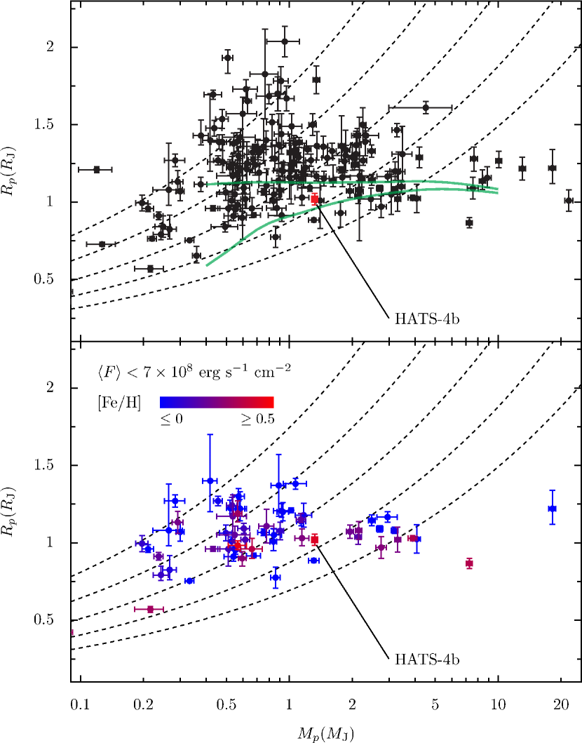
Figure 7.— Top panel: Mass-radius diagram for a large sample of known TEPs (black circles). HATS-4b is indicated by the red square. Overlaid as thick green lines are Fortney et al. (2007) isochrones interpolated to the solar equivalent semi-major axis of HATS-4b for an age of 4.5 Gyr and core masses of 0 (upper) and 100 (lower) $M_{\earth}$. We also overlay isodensity lines for $\rho_{p}=\{0.25,0.5,1,2,4\}$ gr cm^-3 (dashed curves). Data taken from exoplanets.org on Jan 9 2014, adding HATS-3b (Bayliss et al., 2013) and HATS-5b (Zhou et al., 2014a). Bottom panel: Same as top panel but restricted to planets with incoming flux per unit surface area (averaged over the orbit) $\langle F\rangle<7\times 10^{8}$ $\rm erg\,s^{-1}\,cm^{-2}$. The color of the points encodes metallicity, going from blue for $\rm[Fe/H]{}\leq 0$ to red for $\rm[Fe/H]\geq 0.5$ as indicated in the figure.

We have presented in this work the discovery of HATS-4b by the HATSouth survey, which combines data from three stations around the globe with close to optimal longitude separations in order to detect transits. For HATS-4b all of the six HATSouth units contributed to the observations due to it being located in the overlap of two fields that were monitored by the network, resulting in a substantial 33,212 photometric measurements.

The most remarkable properties of the HATS-4 system are the high metallicity of its star and the modest radius of HATS-4b given its mass of $M_{p}\approx 1.32$ $M_{\rm J}$, or equivalently its high density for its mass. The metallicity of HATS-4 makes it more metal rich than $>$99% of all planet hosting stars known to date. We show in the top panel of Figure 7 how HATS-4b compares to all other known TEPs on a mass-radius diagram, while the lower panel shows only planets with irradiation levels $\lesssim$ that of HATS-4b, i.e. $\langle F\rangle<7\times 10^{8}$ $\rm erg\,s^{-1}\,cm^{-2}$. It is immediately clear that HATS-4b is among the most compact known exoplanets in the $\approx$ 1–2 Jupiter mass range, even when restricted to systems that have modest irradiation levels. A straightforward inference from this fact is that HATS-4b is likely to have a significant amount of heavy elements. A comparison with the models of Fortney et al. (2007) suggests a core mass of $\approx$ 75 $M_{\earth}$. Its irradiation level of $\langle F\rangle=6.74\pm 0.44$ $10^{8}$ $\rm erg\,s^{-1}\,cm^{-2}$ is near the level below which planets are found to be not inflated, and thus the uncertainties introduced by any model assumptions as to the relation between the incident flux and the mechanism that produces inflated radii are expected to be minor. While the uncertainties in the models do not allow us to make firm conclusions as to the precise value of the core mass, or indeed if there is a core at all as the heavy elements could be fully mixed in an envelope, the conclusion that HATS-4b is likely to have a significant content of heavy elements can be obtained just by its position close to the lower envelope in the mass-radius diagram of the population of Jupiter mass planets with modest irradiation levels.

The significant heavy element content of HATS-4b may be related to the high metallicity of the host ($\rm[Fe/H]$$=0.43\pm 0.08$). Miller & Fortney (2011) found that for transiting planets with low irradiation levels, systems around stars with high stellar metallicity tend to have a higher mass of heavy elements. The trend presented in Miller & Fortney (2011) has a large scatter though. In the bottom panel of Figure 7 the redder points represent more metal-rich systems. Although none of the redder points appear close to the upper envelope of the distribution, the most compact systems are not exclusively the most metal-rich ones. The heavy element content of a planet probably depends on many factors, including where in the protoplanetary disk it formed, when it formed relative to the disk lifetime, and its detailed migration history, for example if significant migration happened while the disk is still present. Such factors could give rise to a large scatter in any correlation between planet and host star metal fractions. There also appear to be strong exceptions that call into question the existence of a very definite correlation between heavy element content and $\rm[Fe/H]$, such as the very compact CoRoT-13b (Cabrera et al., 2010), which has a host star with $\rm[Fe/H]$ $\approx 0$ and a heavy element content $\approx 200$ $M_{\earth}$. Even though its irradiation level is higher than those of the sample considered by Miller & Fortney (2011), a higher irradiation should result, if anything, in an inflated radius. CoRoT-13 does have a large overabundance of Li (+1.45 dex), so it may be that detailed abundances of host stars are more relevant than overall metallicity when considering correlations with the heavy element content of planets. The tenuousness of the correlation of heavy element content with $\rm[Fe/H]$ is illustrated by the recent analysis of Zhou et al. (2014a) that fitted for linear dependencies of hot Jupiter radii on both planetary equilibrium temperature and $\rm[Fe/H]$, finding that there is no statistically significant correlation with $\rm[Fe/H]$ as would be expected if higher $\rm[Fe/H]$ led tightly to higher heavy element content. As transiting surveys such as HATSouth uncover more systems residing in stars of extreme iron element content such as HATS-4b we will be able to assess with ever more confidence the role of stellar metallicity in determining the heavy element content of exoplanets.

Appendix A Adopted Data Reduction and Analysis Procedures for CORALIE

The CORALIE instrument is a fibre-fed echelle spectrograph mounted on the 1.2m Euler Swiss Telescope at the ESO La Silla Observatory (Queloz et al., 2001a). The resolving power of CORALIE is now $R\approx 60000$ after a refurbishment of the instrument performed in 2007. The full width at half-maximum of an unresolved spectral line is sampled by $\approx$ 3 pixels of the 2k$\times$2k CCD detector. The spectrograph contains two fibers, an object fiber that during science observations is illuminated by the target and a comparison fiber that is simultaneously illuminated either by a wavelength reference lamp to measure instrumental velocity drifts, or by the sky. The echelle grating divides the object spectrum in 71 useful orders which are distributed over the whole CCD, giving spectral coverage of $\approx$ 3000 Å in a single exposure. Only the 48 bluest

The CORALIE reduction procedure adopted by HATSouth observations was briefly described in Penev et al. (2013). Here we describe the pipeline in more detail. The core of the pipeline was written in Python, while some computationally intensive tasks were written in C. The pipeline was developed following a four step structure, which can be identified as: pre-processing, extraction, wavelength calibration, and post-processing. In the following paragraphs we describe each step separately.

A.1. Pre-Proccessing

The pipeline starts with the classification of the different image frames present in a directory according to the FITS header information. The different frames our CORALIE pipeline uses are bias, quartz (fiber flats), ThAr frames (object or comparison fiber illuminated by the wavelength reference lamp) and science frames (in our case, with the object fiber illuminated by a star and the comparison fiber by the wavelength reference lamp). Once the classification is done, master bias and flat frames are constructed by median combining biases and fiber flats. The master bias is used to subtract the bias structure while the master flats are used to trace all echelle orders for both the object and comparison fibres. The latter step relies on order finding and tracing algorithms, which we now describe.

The order finding algorithm starts by median filtering the central column of the master flat with a 45-pixel window. Then, a robust mean and standard-deviation of this baseline-subtracted column is obtained and an order is considered as detected if a given pixel and two consecutive ones have a signal of more than 5 standard deviations from the mean. The positions of these consecutive pixels are saved and then their signals are cross-correlated with a Gaussian in order to find robust pixel positions for the center of the profile of each order at the central column. The process is repeated for adjacent columns, and the centers for each order are finally fitted with a fourth degree polynomial to determine the trace for each order.

A.2. Extraction

Once orders have been traced using the master flat frames we proceed to extract the flux of the science and ThAr frames. For the latter we perform a simple extraction, i.e. just summing the flux in an a region $\pm 3$ pixels around the trace. The same is true of the comparison fiber of the science frames which is illuminated by the ThAr lamp. For the object fiber in the science frames we perform optimal extraction for distorted spectra as presented in Marsh (1989).

A.3. Wavelength Calibration

Wavelength calibration is computed based on the emission lines of the spectrum of a Thorium-Argon (ThAr) lamp. The pipeline only identifies lines contained in the line list presented in Lovis & Pepe (2007). Reference files are created once for every echelle order. In these reference files each line is associated with an approximate pixel position along the trace. The pipeline then fits Gaussians around these zones after determining an offset in pixel space between the positions in the reference file and the lines of a given echelle order in the frame under processing via cross-correlation. The Gaussian means give precise pixel positions of the lines, allowing us to determine the relation between wavelength, pixel and echelle order for each emission line. In the case of blended lines, multiple Gaussians are fitted. An individual wavelength solution is first computed for each echelle order and ThAr lines that deviate significantly from the fit are rejected iteratively until the RMS is below 75 $\rm m\,s^{-1}$. Then a global wavelength solution in the form of an expansion of the grating equation (see §2.6 in Baranne et al., 1996) using Chebyshev polynomials is fitted and more lines are iteratively rejected until the RMS of the global solution is below 100 $\rm m\,s^{-1}$. Our global wavelength solution takes the following form

$$\lambda(x,m)=\frac{1}{m}\sum_{i=0}^{3}\sum_{j=0}^{4}a_{ij}c^{i}(m)c^{j}(x)$$ (A1)

where $x$ and $m$ refers to pixel value and echelle order number respectively, $c^{n}$ denotes the Chebyshev polynomial of order $n$, and $a_{ij}$ are the coefficients that are fitted for to obtain the wavelength solution. The echelle order numbers in CORALIE range from $m_{i}=89$ (reddest) to $m_{f}=159$ (bluest).

Wavelength solutions are first computed for object and comparison fibers of all ThAr calibration frames and each science frame is associated to the closest ThAr frame in time. Then, the pipeline determines the instrumental velocity shift $\delta v$ between the science frame and the associated ThAr frame by fitting a velocity-shifted version of the wavelength solution of the comparison fiber of the associated ThAr frame to the comparison fiber of the science frame. Finally, the object fiber wavelength solution of the associated ThAr frame is applied to the science object fiber shifted by the instrumental velocity shift $\delta v$ computed with the comparison fibers. In general, the instrumental shifts are smaller than 10 $\rm m\,s^{-1}$ on timescales of $\sim$ 1 hour.

A.4. Post-Processing

After obtaining the wavelength calibrated spectrum of a star, the pipeline determines the barycentric correction and applies it to the wavelength solution using routines from the Jet Propulsion Laboratory ephemerides (JPLephem) package. We then apply a fast and robust stellar parameter determination to each stellar spectrum. In order to estimate the stellar parameters ($T_{\rm eff\star}$, $\log{g}$, $\rm[Fe/H]$, $v\sin{i}$) we cross-correlate the observed spectrum against a grid of synthetic spectra of late type stars from Coelho et al. (2005) convolved to the resolution of CORALIE and a set of $v\sin{i}$ values given by $\{0,2.5,5,7.5,10,15,\ldots,45,50\}$ $\rm km\,s^{-1}$. First a set of atmospheric parameters is determined as a starting point by ignoring any rotation and searching for the model that produces the highest cross-correlation using only the Mg triplet region. We use a coarse grid of models for this initial step ($\Delta T_{\rm eff\star}=1000$ K, $\Delta\log{g}=1.0$, $\Delta\rm[Fe/H]=1.0$). A new cross-correlation function (CCF) between the observed spectrum and the model with the starting point parameters is then computed using a wider spectral region (4800 Å– 6200 Å). From this CCF we estimate RV and $v\sin{i}$ values using the peak position and width of the CCF, respectively. New $T_{\rm eff\star}$, $\log{g}$ and $\rm[Fe/H]$ values are then estimated by fixing $v\sin{i}$ to the closest value present in our grid and searching for the set of parameters that gives the highest cross-correlation, and the new CCF is used to estimate new values of RV and $v\sin{i}$. This procedure is continued until convergence on stellar parameters is reached. For high S/N spectra, uncertainties of this procedure are typically 200 K in $T_{\rm eff\star}$, 0.3 dex in $\log{g}$, 0.2 dex in $\rm[Fe/H]$ and 2 $\rm km\,s^{-1}$ in $v\sin{i}$. These uncertainties were estimated from observations of stars with known stellar parameters from the literature. Results of our stellar parameter estimation procedure are obtained in about 2 minutes using a standard laptop Fast and robust atmospheric parameters are estimated in order to make efficient use of the available observing time because in this way some false positives or troublesome systems, such as fast rotators and giants, can be identified on the fly during the follow-up process.

The radial velocity of the spectrum is computed using the cross-correlation technique against a binary mask (Baranne et al., 1996) which depends on the spectral type. The available masks are for G2, K5 and M5, and are the same ones used by the HARPS (Mayor et al., 2003) data reduction system but with the transparent regions made wider given that the resolution of CORALIE is $\approx$ 0.5 times that of HARPS. If a target is being observed for the first time, first a query to the SIMBAD database is made to see if the spectral type is known and otherwise our estimate of $T_{\rm eff\star}$ is used to assign the mask to calculate the radial velocity. Future observations of the same target will use always this same mask to compute the radial velocity. The CCF is computed for each echelle order and then a weighted sum is applied to get the final CCF. Weights are given by the mean S/N on the continuum for each echelle order. A simple Gaussian is fitted to the CCF, and the mean is taken as the RV of the spectrum. The pipeline also infers the presence of moonlight contamination in the CCF. If there is a secondary peak on the CCF due to the moon, the pipeline computes the position and width of this peak and fits for the intensity to correct the RV determination. Bisector spans are also measured using the CCF peak as described in Queloz et al. (2001b). Uncertainties on RV and bisector span are determined from the width of the CCF and the mean S/N close to the Mg triplet zone using empirical scaling relations (as in, e.g., Queloz, 1995) whose parameters are determined using Monte Carlo simulations where Gaussian noise is artificially added to high S/N spectra. The exact equations used to estimate the errors are

$$\sigma_{\rm RV}=b+\frac{a(1.6+0.2\sigma_{\rm ccf})}{{\rm SN}_{5130}}$$ (A2)

$$\sigma_{\rm BS}=\frac{d}{{\rm SN}_{5130}}+c$$ (A3)

where $a,b,c,d$ are the coefficients obtained via the Monte Carlo simulations and depend on the applied mask, ${\rm SN}_{5130}$ is the continuum S/N at 5130 Å and $\sigma_{\rm ccf}$ is the dispersion of the Gaussian fit to the CCF. For illustration, the values of the coefficients for the G2 mask are $a=0.06544,b=0.00146,c=0.00181$ and $d=0.24416$. If the estimated uncertainty $\sigma_{\rm RV}<9\,\rm m\,s^{-1}$ we assign it a value of 9 $\rm m\,s^{-1}$ given that the long-term radial velocity precision we achieve is $\approx$ 9 $\rm m\,s^{-1}$ over a timescale of several years. We determined this value by monitoring 3 radial velocity standard stars (HD72673, HD157347, HD32147) starting around 2010. Figure 8 shows the radial velocity time series for all the CORALIE measurements we have taken of the standards, whose spectra have ${\rm SN}_{5130}$ in the range $\sim$ 50–150.

Figure 8.— Radial velocity $v_{r}$ time series for the 3 RV standard stars we have monitored with CORALIE. In each panel we show the name of the standard and the root mean square deviation around the mean RV ($\langle v_{r}\rangle$). We conclude from these data that our long-term stability is $\approx$ 9 $\rm m\,s^{-1}$.

References

- Albrecht et al. (2012) Albrecht, S., Winn, J. N., Johnson, J. A., et al. 2012, ApJ, 757, 18
- Bakos et al. (2007) Bakos, G. Á., Kovács, G., Torres, G., et al. 2007, ApJ, 670, 826
- Bakos et al. (2010) Bakos, G. Á., Torres, G., Pál, A., et al. 2010, ApJ, 710, 1724
- Bakos et al. (2013) Bakos, G. Á., Csubry, Z., Penev, K., et al. 2013, PASP, 125, 154
- Baranne et al. (1996) Baranne, A., Queloz, D., Mayor, M., et al. 1996, A&AS, 119, 373
- Bayliss et al. (2013) Bayliss, D., Zhou, G., Penev, K., et al. 2013, AJ, 146, 113
- Boué et al. (2013) Boué, G., Montalto, M., Boisse, I., Oshagh, M., & Santos, N. C. 2013, A&A, 550, A53
- Buchhave et al. (2012) Buchhave, L. A., Latham, D. W., Johansen, A., et al. 2012, Nature, 486, 375
- Burrows et al. (2007) Burrows, A., Hubeny, I., Budaj, J., & Hubbard, W. B. 2007, ApJ, 661, 502
- Butler et al. (1996) Butler, R. P., Marcy, G. W., Williams, E., et al. 1996, PASP, 108, 500
- Cabrera et al. (2010) Cabrera, J., Bruntt, H., Ollivier, M., et al. 2010, A&A, 522, A110
- Claret (2004) Claret, A. 2004, A&A, 428, 1001
- Claret & Bloemen (2011) Claret, A., & Bloemen, S. 2011, A&A, 529, A75
- Coelho et al. (2005) Coelho, P., Barbuy, B., Meléndez, J., Schiavon, R. P., & Castilho, B. V. 2005, A&A, 443, 735
- Crane et al. (2010) Crane, J. D., Shectman, S. A., Butler, R. P., et al. 2010, in Society of Photo-Optical Instrumentation Engineers (SPIE) Conference Series, Vol. 7735, Society of Photo-Optical Instrumentation Engineers (SPIE) Conference Series
- Demory & Seager (2011) Demory, B.-O., & Seager, S. 2011, ApJS, 197, 12
- Dopita et al. (2007) Dopita, M., Hart, J., McGregor, P., et al. 2007, Ap&SS, 310, 255
- Fortney et al. (2007) Fortney, J. J., Marley, M. S., & Barnes, J. W. 2007, ApJ, 659, 1661
- Girardi et al. (2000) Girardi, L., Bressan, A., Bertelli, G., & Chiosi, C. 2000, A&AS, 141, 371
- Gray (2005) Gray, D. F. 2005, The Observation and Analysis of Stellar Photospheres
- Guillot et al. (2006) Guillot, T., Santos, N. C., Pont, F., et al. 2006, A&A, 453, L21
- Hansen & Barman (2007) Hansen, B. M. S., & Barman, T. 2007, ApJ, 671, 861
- Hartman et al. (2011a) Hartman, J. D., Bakos, G. Á., Sato, B., et al. 2011a, ApJ, 726, 52
- Hartman et al. (2011b) Hartman, J. D., Bakos, G. Á., Torres, G., et al. 2011b, ApJ, 742, 59
- Henden et al. (2009) Henden, A. A., Welch, D. L., Terrell, D., & Levine, S. E. 2009, in American Astronomical Society Meeting Abstracts, Vol. 214, American Astronomical Society Meeting Abstracts #214, #407.02
- Husser et al. (2013) Husser, T.-O., Wende-von Berg, S., Dreizler, S., et al. 2013, A&A, 553, A6
- Kaufer & Pasquini (1998) Kaufer, A., & Pasquini, L. 1998, in Society of Photo-Optical Instrumentation Engineers (SPIE) Conference Series, Vol. 3355, Optical Astronomical Instrumentation, ed. S. D’Odorico, 844–854
- Kovács et al. (2002) Kovács, G., Zucker, S., & Mazeh, T. 2002, A&A, 391, 369
- Lovis & Pepe (2007) Lovis, C., & Pepe, F. 2007, A&A, 468, 1115
- Maldonado et al. (2012) Maldonado, J., Eiroa, C., Villaver, E., Montesinos, B., & Mora, A. 2012, A&A, 541, A40
- Mandel & Agol (2002) Mandel, K., & Agol, E. 2002, ApJ, 580, L171
- Marsh (1989) Marsh, T. R. 1989, PASP, 101, 1032
- Mayor et al. (2003) Mayor, M., Pepe, F., Queloz, D., et al. 2003, The Messenger, 114, 20
- Miller & Fortney (2011) Miller, N., & Fortney, J. J. 2011, ApJ, 736, L29
- Mohler-Fischer et al. (2013) Mohler-Fischer, M., Mancini, L., Hartman, J. D., et al. 2013, A&A, 558, A55
- Noguchi et al. (2002) Noguchi, K., Aoki, W., Kawanomoto, S., et al. 2002, PASJ, 54, 855
- Pál (2009) Pál, A. 2009, MNRAS, 396, 1737
- Penev et al. (2013) Penev, K., Bakos, G. Á., Bayliss, D., et al. 2013, AJ, 145, 5
- Queloz (1995) Queloz, D. 1995, in IAU Symposium, Vol. 167, New Developments in Array Technology and Applications, ed. A. G. D. Philip, K. Janes, & A. R. Upgren, 221
- Queloz et al. (2001a) Queloz, D., Mayor, M., Udry, S., et al. 2001a, The Messenger, 105, 1
- Queloz et al. (2001b) Queloz, D., Henry, G. W., Sivan, J. P., et al. 2001b, A&A, 379, 279
- Sato et al. (2002) Sato, B., Kambe, E., Takeda, Y., Izumiura, H., & Ando, H. 2002, PASJ, 54, 873
- Sato et al. (2005) Sato, B., Fischer, D. A., Henry, G. W., et al. 2005, ApJ, 633, 465
- Sato et al. (2012) Sato, B., Hartman, J. D., Bakos, G. Á., et al. 2012, PASJ, 64, 97
- Sozzetti et al. (2007) Sozzetti, A., Torres, G., Charbonneau, D., et al. 2007, ApJ, 664, 1190
- Yi et al. (2001) Yi, S., Demarque, P., Kim, Y.-C., et al. 2001, ApJS, 136, 417
- Zhou et al. (2014a) Zhou, G., Bayliss, D., Penev, K., et al. 2014a, ArXiv e-prints arXiv:1401.1582Z
- Zhou et al. (2014b) Zhou, G., Bayliss, D., Hartman, J. D., et al. 2014b, MNRAS, 437, 2831