The ”True” Widom Line for a Square-Well System

Abstract

In the present paper we propose the van der Waals-like model, which allows a purely analytical study of fluid properties including the equation of state, phase behavior and supercritical fluctuations. We take a square-well system as an example and calculate its liquid - gas transition line and supercritical fluctuations. Employing this model allows us to calculate not only the thermodynamic response functions (isothermal compressibility $\beta_{T}$, isobaric heat capacity $C_{P}$, density fluctuations $\zeta_{T}$, and thermal expansion coefficient $\alpha_{T}$), but also the correlation length in the fluid $\xi$. It is shown that the bunch of extrema widens rapidly upon departure from the critical point. It seems that the Widom line defined in this way cannot be considered as a real boundary that divides the supercritical region into the gaslike and liquidlike regions. As it has been shown recently, the new dynamic line on the phase diagram in the supercritical region, namely the Frenkel line, can be used for this purpose.

In recent years, a growing attention has been given to the investigation of properties of supercritical liquids. This interest is mainly due to the fact, that supercritical fluids are widely used in industrial processes. Their behavior away from the critical point is therefore an important practical question because it might affect their applicability in the considered technological process appl_supp . Theoretical aspects of the physics of supercritical fluid are of particular interest as well.

The liquid-gas phase equilibrium curve in the $P-T$ plane ends at the critical point. At pressures and temperatures above the critical ones ($P>P_{c}$ and $T>T_{c}$), the properties of a substance in the isotherms and isobars vary continuously, and it is commonly said that the substance is in its supercritical fluid state, when there is no difference between liquid and gas. From the physical point of view, the $P,T$ region near the critical point, where anomalous behavior of the majority of characteristics is observed (the so-called critical behavior) is of prime interest stanley_book . The correlation length of thermodynamic fluctuations diverges at the critical point stanley_book . One can also observe a critical behavior of the thermodynamic response functions, which are defined as second derivatives of the corresponding thermodynamic potentials; such as the compressibility coefficient $\beta_{T}$, thermal expansion coefficient $\alpha_{P}$, and heat capacity $C_{P}$. These quantities pass through their maxima during pressure or temperature variations and diverge as the critical point is approached. Near the critical point, the positions of the maxima of these values in the $T,P$-plane are close to each other. The same is true for the density fluctuations, the speed of sound, thermal conductivity, etc. Therefore, in the supercritical region, there is the whole set of the lines of extrema of various thermodynamic parameters. The lines of the maxima for different response functions asymptotically approach one another as the critical point is approached, because all response functions can be expressed in terms of the correlation length. This asymptotic line is sometimes called the ”Widom line” and is often regarded as an extension of the coexistence line into the ”one-phase region” pnas2005 . The Widom lines for the gas-liquid and liquid-liquid phase transitions have been investigated extensively pnas2005 ; poole ; fr_st ; mcm_st ; bryk1 ; bryk2 ; jpcb ; br_jcp ; br_ufn ; gallo_jcp ; riem ; may .

Because of the lack of a theoretical method for constructing the Widom line, based on the extremum of the correlation length, the locus of extrema of the constant-pressure specific heat $C_{P}$ was often used as an estimation for the Widom line. In Refs. jpcb ; br_ufn , using the computer simulations, the locus of extrema (ridges) for the heat capacity, thermal expansion coefficient, compressibility, and density fluctuations for model particle systems with Lennard-Jones (LJ) potential in the supercritical region have been obtained. It was found that the ridges for different thermodynamic values virtually merge into a single Widom line at $T<1.1T_{c}$ and $P<1.5P_{c}$ and become almost completely smeared at $T<2.5T_{c}$ and $P<10P_{c}$, where $T_{c}$ and $P_{c}$ are the critical temperature and pressure. The analytical expressions for the extrema of the heat capacity, thermal expansion coefficient, compressibility, density fluctuation, and sound velocity in the supercritical region were obtained in Refs. br_jcp ; br_ufn in the framework of the van der Waals (vdW) model. It was found that the ridges for different thermodynamic values virtually merge into a single Widom line only at $T<1.07T_{c},P<1.25P_{c}$ and become smeared at $T<2T_{c},P<5P_{c}$. However, in both of the studies, the estimation of the Widom line is unsatisfactory because it is a priori unclear how far from the critical point the lines of extrema of response functions follow the exact Widom line, determined by the maximum of the correlation length.

Recently it was proposed to construct the Widom line by using the approach based on Riemannian geometry riem . Previously it was supposed that there is a relation between the Riemannian thermodynamic scalar curvature $R$ of the thermodynamic metric and the volume of the correlation length $\xi$, i.e., $|R|\propto\xi^{3}$ riem2 . Consequently, the locus of the maximum of $|R|$ describes the locus of the Widom line. In Ref. riem this approach was applied to a van der Waals (vdW) fluid, while in may it was used for constructing the Widom line for the LJ fluid.

It is of great interest to develop a simple vdW-like model which can represent a liquid-gas transition and the Widom line, and can be solved analytically. In this case it would be possible to analyze the relation between the”true” Widom line, determined from the correlation function, and the lines of extrema of response functions.

We define the model using the approximation for the direct correlation function book of the hard-core system, suggested by Lovett lovett (see also RT1 ; RT2 ; TMF ):

$$c(r)=\left\{\begin{array}[]{ll}c_{HS}(r),&r\leq d\\ -\frac{\phi(r)}{k_{B}T},&r>d\end{array}\right.,$$ (1)

where $c_{HS}(r)$ is the hard spheres direct correlation function and $\phi(r)$ is the attractive part of the potential. This should be a good approximation when $-\frac{\phi(r)}{k_{B}T}$ is small. The approximation, though rough, is similar in spirit to the mean spherical model approximation which has been found to be a good approximation in many cases book . Such an approximation formulated directly in terms of $c(r)$ is particularly convenient for the formulation of the Widom line, as it will be shown below. This approximation is especcially convenient for direct calculation of the correlation length in the fluid $\xi$.

Although the method we use is a general tool for liquids, we consider the so-called square well (SW) system as more specific. One can easily generalize the results to other systems. The square well system is a system of particles interacting via the following potential:

$$\Phi(r)=\left\{\begin{array}[]{lll}\infty,&r\leq d\\ -\varepsilon,&d<r\leq\sigma\\ 0,&r>\sigma\end{array}\right..$$ (2)

Although this system is not very realistic, it can serve as a generic example of a simple liquid. Below we consider the SW system with $\sigma=1.35d$. In this case, Eq. (1) has the form:

$$c(r)=\left\{\begin{array}[]{lll}c_{HS}(r),&r\leq d\\ \frac{\varepsilon}{k_{B}T},&d<r\leq\sigma\\ 0,&r>\sigma\end{array}\right.$$ (3)

We use the Percus-Yevick approximation book for $c_{HS}$:

$$c_{HS}(r)=-\lambda_{1}-\pi\rho\lambda_{2}r-\frac{\pi}{12}\rho\lambda_{1}r^{3},$$ (4)

where

$$\lambda_{1}=\frac{(1+2\eta)^{2}}{(1-\eta)^{4}}$$

and

$$\lambda_{2}=\frac{-d^{2}(1+1/2\eta)^{2}}{(1-\eta)^{4}}.$$

$\eta$ is the packing fraction $\eta=\frac{\pi}{6}\rho d^{3}$.

The direct correlation function can be used to obtain the isothermal compressibility:

$$\frac{1}{k_{B}T}\left(\frac{\partial P}{\partial\rho}\right)_{T}=1-\rho\int d\textbf{r}c(r).$$ (5)

Taking into account, that the system is isotropic, and using Eq. (4), one obtains:

$$\frac{1}{k_{B}T}\left(\frac{\partial P}{\partial\rho}\right)_{T}=\lambda_{1}-\frac{8\varepsilon}{k_{B}T}\eta\Delta,$$ (6)

where $\Delta=(\sigma^{3}-d^{3})/d^{3}$.

The integration of Eq. (6) gives the equation of state (EoS) for the SW system:

$$\tilde{P}=\tilde{T}\cdot\frac{\eta+\eta^{2}+\eta^{3}}{(1-\eta)^{3}}-4\Delta\eta^{2},$$ (7)

where $\tilde{P}=P\cdot\frac{\pi d^{3}}{6\varepsilon}$ and $\tilde{T}=k_{B}T/\varepsilon$. Further in the paper we will use only these scaled units, omitting the tilde mark.

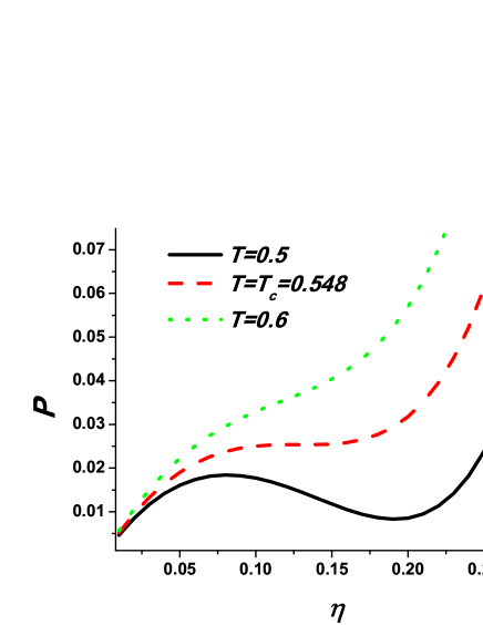
Figure 1: (Color online) Three isotherms for SW system: below the critical temperature $T_{c}$, at $T=T_{c}$ and above $T_{c}$.

Fig. 1 shows three isotherms for the SW system: below the critical temperature $T_{c}$, at $T=T_{c}$ and above $T_{c}$. The critical point can be determined from the following conditions:

$$\frac{\partial P}{\partial\eta}=T\cdot\frac{(1+2\eta)^{2}}{(1-\eta)^{4}}-8\Delta\eta$$ (8)

and

$$\frac{\partial^{2}P}{\partial\eta^{2}}=T\cdot\frac{8+20\eta+8\eta^{2}}{(1-\eta)^{5}}-8\Delta.$$ (9)

Rewriting these equations in the following form

$$T(1+4\eta+4\eta^{2})=8\Delta\eta(1-\eta)^{4}$$

$$T(8+20\eta+8\eta^{2})=8\Delta(1-\eta)^{5},$$ (10)

we obtain the following equation for the critical packing fraction:

$$1-5\eta-20\eta^{2}-12\eta^{3}=0.$$ (11)

From this equation one can get the critical packing fraction $\eta_{c}=0.12867...$. It is important to emphasize that in approximation (3) the critical density is fully determined by the hard core diameter $d$ and does not depend on the well width $\sigma$.

For the critical temperature one obtains:

$$T_{c}=\frac{8\Delta\eta_{c}(1-\eta_{c})^{4}}{(1+2\eta_{c})^{2}}.$$ (12)

Using the value for the critical packing fraction obtained above one can write $T_{c}=0.375312\Delta$. For the system with $\sigma=1.35d$, which we study here, $T_{c}=0.548$.

The liquid - gas (LG) transition line can be obtained by the Maxwell construction. Figs. 4 ((a) and (b)) show the LG curve in the $\eta-T$ and $P-T$ planes.

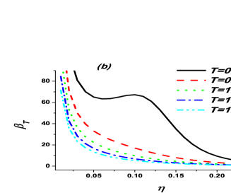
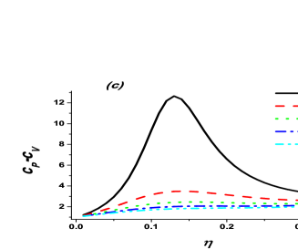
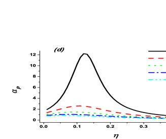
Figure 2: (Color online) (a) Density fluctuations $\zeta_{T}$, (b) isothermal compressibility $\beta_{T}$, (c) heat capacity $c_{P}$, and (d) isobaric thermal expansion coefficient $\alpha_{P}$ along several isotherms.

It is well known that close to the critical point, many thermodynamic functions have maxima. Here we calculate the locations of maxima of different thermodynamic functions in the framework of the method employed. The real advantage of this method is that it allows us to calculate the correlation length $\xi$, i.e. we are able to compare all the definitions of the Widom line in framework of the purely analytical study of the same system.

Isothermal density fluctuations are defined as $\zeta_{T}=T\left(\frac{\partial\rho}{\partial P}\right)_{T}$. From the equations given above one obtains:

$$\zeta_{T}=T\frac{\partial\eta}{\partial P}=\frac{T(1-\eta)^{4}}{T(1+2\eta)^{2}-8\Delta\eta(1-\eta)^{4}}.$$ (13)

Fig. 2 (a) shows the density fluctuations along several isotherms. The $\zeta_{T}$ maxima along isotherms are determined from the following equation:

$$T=\frac{2\Delta(1-\eta)^{5}}{2+5\eta+2\eta^{2}}.$$ (14)

The isothermal compressibility is defined as $\beta_{T}=-\frac{1}{V}\left(\frac{\partial V}{\partial P}\right)_{T}$. Rewriting it in terms of $\eta$, one obtains:

$$\beta_{T}=\frac{1}{\eta}\left(\frac{\partial\eta}{\partial P}\right)_{T}=\frac{1}{\eta}\frac{(1-\eta)^{4}}{T(1+2\eta)^{2}-8\Delta\eta(1-\eta)^{4}}.$$ (15)

Fig. 2 (b) shows the compressibilities $\beta_{T}$ along several isotherms. The corresponding maxima are obtained from the equation:

$$T=\frac{16\Delta\eta(1-\eta)^{5}}{1+11\eta+20\eta^{2}+4\eta^{3}}.$$ (16)

The heat capacity $C_{P}$ can be calculated from the formula:

$$C_{P}-C_{V}=-T\frac{\left(\frac{\partial P}{\partial T}\right)^{2}_{V}}{\left(\frac{\partial P}{\partial V}\right)_{T}}.$$ (17)

In terms of $\eta$ this formula is

$$C_{P}-C_{V}=\frac{T(1+\eta+\eta^{2})^{2}}{(1-\eta)^{2}(T(1+2\eta)^{2}-8\Delta\eta(1-\eta)^{4})}.$$ (18)

Some examples of the heat capacities along isotherms are shown in Fig. 2 (c). The corresponding maxima can be calculated from the equation:

$$T=\frac{4\Delta(1-\eta)^{4}(-1+8\eta+8\eta^{2}+3\eta^{3})}{3\eta(2+5\eta+2\eta^{2})}.$$ (19)

Taking into account that, as in the case of the vdW model stanley_book , $C_{V}$ above the critical point is equal to the ideal gas value, Eq. (19) corresponds to the line of the supercritical maxima of $C_{P}$. However, in contrast to the vdW model, where the line of $C_{P}$ maxima is located along the critical isochore br_jcp , in this model the supercritical behavior of $C_{P}$ (see Fig. 3) is similar to that in the case of the LJ fluid jpcb ; may .

The isobaric thermal expansion coefficient is $\alpha_{P}=-\frac{1}{V}\left(\frac{\partial V}{\partial T}\right)_{P}$. Using the EoS (7), one obtains

$$\alpha_{P}=\frac{1}{\eta}\left(\frac{\partial\eta}{\partial T}\right)_{P}=\frac{(1+\eta+\eta^{2})(1-\eta)}{T(1+2\eta)^{2}-8\Delta\eta(1-\eta)^{4}}.$$ (20)

Some examples of the $\alpha_{P}$ behavior along isotherms are shown in Fig. 2 (d). The corresponding isothermal maxima are given by the equation

$$T=\frac{-8\Delta(1-\eta)^{4}(-1+4\eta+4\eta^{2}+2\eta^{3})}{4+8\eta+3\eta^{2}+8\eta^{3}+4\eta^{4}}.$$ (21)

The correlation length can be calculated in the following way book :

$$\xi^{2}=\frac{R^{2}}{1-\rho\tilde{C}_{0}(T)},$$ (22)

where

$$R^{2}=\frac{\rho}{6}\int c(r)r^{2}d\textbf{r},$$ (23)

and

$$\tilde{C}_{0}(T)=\int c(r)d\textbf{r}.$$ (24)

Using the formulas for the direct correlation function book , one can write:

$$1-\rho\tilde{C}_{0}(T)=\lambda_{1}-\frac{8\eta\Delta}{T}.$$ (25)

Substituting this equation into the one for $R^{2}$, one obtains:

$$R^{2}=\frac{\eta d^{2}}{20}\left[\frac{-16+11\eta-4\eta^{2}}{(1-\eta)^{4}}+\frac{16\Delta^{\prime}}{T}\right],$$ (26)

where $\Delta^{\prime}=(\sigma^{5}-d^{5})/d^{5}$.

Finally, for the correlation length one obtains:

$$\tilde{\xi}^{2}=\frac{\xi^{2}}{d^{2}}=\frac{1}{20}\frac{T(-16\eta+11\eta^{2}-4\eta^{3})+16\eta\Delta^{\prime}(1-\eta)^{4}}{T(1+2\eta)^{2}-8\Delta\eta(1-\eta)^{4}}.$$ (27)

Examples of the correlation length along several isotherms are given in Fig. 3. The maxima of the correlation length can be calculated as the solutions of the following equation:

$$4\Delta\eta^{2}(1-\eta)^{3}(-53+25\eta-8\eta^{2})+$$ (28)

$$+ 8\Delta^{\prime}(1-\eta)^{3}(-1+5\eta+20\eta^{2}+12\eta^{3})+$$

$$+ \ T(8-11\eta-48\eta^{2}+16\eta^{3}+8\eta^{4})=0.$$

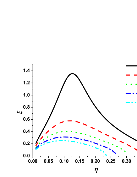
Figure 3: (Color online) Correlation length $\xi$ along several isotherms.

Fig. 4(a) shows the LG curve and the points of maxima of all the quantities described above. One can see, that the curves of maxima of different thermodynamic functions quickly diverge, and even rather close to the critical point, one cannot consider the location of the maxima as a single curve. They actually represent a bunch of curves in the $\eta-T$ plane.

In particular, one can see that the correlation length maxima are located between the $\alpha_{P}$ and $C_{P}$ maxima, and even the qualitative behavior of the maxima of correlation length is opposite to that of the heat capacity in the $\eta-T$ plane.

In Fig. 4(b), the behaviors of maxima of the isothermal compressibility $\beta_{T}$, isobaric heat capacity $C_{P}$, density fluctuations $\zeta_{T}$, thermal expansion coefficient $\alpha_{T}$, and correlation length $\xi$ at constant temperature are shown in the $P-T$ plane. One can see again, that the bunch of ridges merges into a single line in the very vicinity of the critical point and widens rapidly upon departure from the critical point. If the Widom line is defined with the help of the correlation function $\xi$, then the Widom line will not follow the slope of any response function extrema, except in the very close vicinity of the critical point.

It is interesting to note that the sequence of the $\xi$, $\beta_{T}$, $C_{P}$, $\zeta_{T}$, and $\alpha_{T}$ extrema in Fig. 4 is the same as the corresponding sequence for the vdW and LJ fluids jpcb ; br_jcp ; may . It seems that the similar behavior of the correlation length maxima line in our model and the corresponding lines obtained in may may be considered as an evidence of the universality of a particular location of the ”true” Widom line.

It seems that the Widom line defined in this way cannot be used as a single boundary that separates the supercritical region into the gaslike and liquidlike regions. For this purpose, a new dynamic line on the phase diagram in the supercritical region, namely the Frenkel line has been proposed recently br_ufn ; br_jl ; br_pre ; br_jcp1 ; br_prl . The intersection of this line corresponds to radical changes of system properties. Liquids in this region exist in two qualitatively different states: ”rigid” and ”nonrigid” liquids. The rigid to nonrigid transition corresponds to the condition $\tau\approx\tau_{0}$, where $\tau$ is the liquid relaxation time and $\tau_{0}$ is the minimal period of transverse quasiharmonic waves. This condition defines a new dynamic crossover line on the phase diagram and corresponds to the loss of shear stiffness of a liquid at all available frequencies and, consequently, to qualitative changes in many properties of the liquid. In contrast to the Widom line that exists only near the critical point, the new dynamic line is universal. It separates two liquid states at arbitrarily high pressure and temperature and exists in systems where the liquid-gas transition and the critical point are absent altogether. The location of the line can be rigorously and quantitatively established on the basis of the velocity autocorrelation function and mean-square displacements. It was also shown that the positive sound dispersion disappears in the vicinity of the Frenkel line bryk2 ; br_jl ; br_pre ; br_jcp1 ; br_prl .

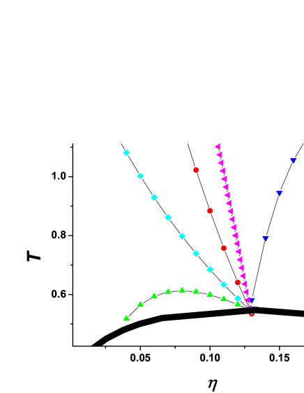
Figure 4: (Color online) Location of maxima of different thermodynamic quantities close to the LG curve (a) in the $\eta-T$ and (b) $P-T$ planes.

In conclusion, in the present paper we propose the van der Waals-like model which allows a purely analytical study of fluid properties including the equation of state, phase behavior and supercritical fluctuations. We take a square-well system as an example and calculate its liquid - gas transition line and supercritical fluctuations. Employing this model allows us to calculate the correlation length in the fluid $\xi$, isothermal compressibility $\beta_{T}$, the isobaric heat capacity $C_{P}$, density fluctuations $\zeta_{T}$, and thermal expansion coefficient $\alpha_{T}$. It is shown that, in accordance with our recent results obtained for Lennard-Jones and van der Waals liquids jpcb ; br_jcp , the bunch of extrema merges into a single line in the very close vicinity of the critical point and widens rapidly upon departure from the critical point. If the ”true” Widom line is defined with the aid of the correlation function $\xi$, one can see that the Widom line does not follow the slope of any response function extrema except those located in the very close vicinity of the critical point. It seems that the Widom line defined in this way cannot be used as the boundary that separates the supercritical region into the gaslike and liquidlike regions. As it has been shown recently, a new dynamic line on the phase diagram in the supercritical region, namely the Frenkel line, can be used for this purpose br_ufn ; br_jl ; br_pre ; br_jcp1 ; br_prl .

- (1) Kiran E., Debenedetti P. G., Peters J., Eds. Supercritical Fluids. Fundamentals and Applications (NATO Science Series E: Applied Sciences 366, Kluwer: Boston, 2000).
- (2) Stanley H. E., Introduction to Phase Transitions and Critical Phenomena (Oxford University Press: Oxford, U.K., 1971).
- (3) Xu L., Kumar P., Buldyrev S. V., Chen S.-H., Poole P. H., Sciortino F., and Stanley H. E., Proc. Natl. Acad. Sci. U.S.A. 2005, 102,16558.
- (4) Poole P. H., Becker S. R., Sciortino F., and Starr F. W., J. Phys. Chem. B 2011, 115, 14176 .
- (5) Franzese G. and Stanley H. E., J. Phys.: Condens. Matter 2007,19, 205126 .
- (6) McMillan P. F. and Stanley E. H., Nat. Phys. 2010, 6, 479 .
- (7) Simeoni G. G., Bryk T., Gorelli F. A., Krisch M., Ruocco G., Santoro M., and Scopigno T., Nat. Phys. 2010, 6, 503.
- (8) Gorelli F. A., Bryk T., Krisch M., Ruocco G., Santoro M., and Scopigno T., Sci. Rep. 2013, 3, 1203.
- (9) Brazhkin V. V., Fomin Yu. D., Lyapin A. G., Ryzhov V. N., and Tsiok E. N., J. Phys. Chem. B 2011, 115, 14112.
- (10) Brazhkin V. V. and Ryzhov V. N., J. Chem. Phys. 2011, 135, 084503.
- (11) Brazhkin V.V., Lyapin A. G., Ryzhov V. N., Trachenko K., Fomin Yu. D., and Tsiok E. N., Usp. Fiz. Nauk 2012, 182, 1137 [Sov. Phys. Usp. 2012, 55, 1061].
- (12) Gallo P., Corradini D., and Rovere M., J. Chem. Phys. 2013, 139, 204503.
- (13) Ruppeiner G., Sahay A., Sarkar T., and Sengupta G., Phys. Rev. E 2012, 86, 052103.
- (14) May H.-O. and Mausbach P., Phys. Rev. E 2012, 85, 031201.
- (15) Ruppeiner G., Rev. Mod. Phys. 1995, 67, 605; 1996, 68, 313(E).
- (16) Hansen J. P., McDonald I. R., Theory of simple liquids (Academic Press, 1986).
- (17) Lovett R., J. Chem. Phys. 1977, 66, 1225.
- (18) Ryzhov V. N. and Tareyeva E. E., Physica A 2002, 314, 396.
- (19) Ryzhov V. N. and Tareyeva E. E., Theor. Math. Phys. 2002, 130, 101 (DOI: 10.1023/A:1013884616321).
- (20) Ryzhov V. N., Tareyeva E. E., and Fomin Yu. D., Theor. Math. Phys. 2011, 167, 645.
- (21) Brazhkin V. V., Fomin Yu. D., Lyapin A. G., Ryzhov V. N., and Trachenko K., Pis ma Zh. Eksp. Teor. Fiz. 2012, 95, 179 [JETP Lett. 2012, 95, 164].
- (22) Brazhkin V. V., Fomin Yu. D., Lyapin A. G., Ryzhov V. N., and Trachenko K., Phys. Rev. E 2012, 85, 031203.
- (23) Bolmatov Dima, Brazhkin V. V., Fomin Yu. D., Ryzhov V. N., and Trachenko K., J. Chem. Phys. 2013, 139, 234501.
- (24) Brazhkin V. V., Fomin Yu. D., Lyapin A. G., Ryzhov V. N., Tsiok E. N., and Trachenko Kostya, Phys. Rev. Lett. 2013, 111, 145901.