Order of wetting transitions in electrolyte solutions
Ingrid Ibagon
ingrid@is.mpg.deMarkus Bier
bier@is.mpg.deS. Dietrich
Max-Planck-Institut für Intelligente Systeme,
Heisenbergstr. 3,
70569 Stuttgart,
Germany and
IV. Institut für Theoretische Physik,
Universität Stuttgart,
Pfaffenwaldring 57,
70569 Stuttgart,
Germany
Abstract
For wetting films in dilute electrolyte solutions close to charged walls we present analytic
expressions for their effective interface potentials. The analysis
of these expressions renders the conditions under which corresponding wetting transitions
can be first- or second-order. Within mean field theory we consider two models, one with short- and
one
with long-ranged solvent-solvent and solvent-wall interactions. The analytic results
reveal in a transparent way that wetting transitions in electrolyte solutions, which occur far away
from their critical point (i.e., the bulk correlation length is less than half of the Debye length)
are always first-order if the solvent-solvent and solvent-wall interactions are
short-ranged.
In contrast, wetting transitions close to the bulk critical point of the solvent (i.e., the
bulk correlation length is larger than the Debye length) exhibit the same wetting behavior as the
pure,
i.e., salt-free, solvent. If the salt-free solvent is governed by long-ranged solvent-solvent as
well as long-ranged solvent-wall interactions and exhibits critical wetting, adding salt can cause
the occurrence of an ion-induced first-order thin-thick transition which precedes the subsequent
continuous wetting as for the salt-free solvent.
I Introduction
Recent theoretical studies of wetting phenomena in electrolyte solutions near charged walls have
focused on analyzing the influence of salt and surface charge density on the wetting behavior of
solvents Denesyuk2003 ; Denesyuk2004 ; Oleksy2009 ; Oleksy2010 ; Ibagon . The corresponding models
share
certain common features such as the short range of the underlying non-electrostatic interaction
potentials and the mean-field character of the approaches. The model studied in Refs.
Denesyuk2003 ; Denesyuk2004 combines Cahn’s phenomenological theory for the solvent with
the Poisson-Boltzmann theory for the ions. Within this model, ions and solvent molecules are
completely
decoupled. On the other hand, in Ref. Oleksy2009 the solvent and the ions are modeled as
hard spheres with Yukawa attraction between solvent-solvent, solvent-ion, and ion-ion pairs as well
as
Coulomb
interactions between ions. The model was studied by using classic density functional theory (DFT)
Evans . Subsequently, the model used in Ref. Oleksy2010 includes the polar nature of
the
solvent explicitly, representing its molecules by dipolar hard spheres. In Ref. Ibagon a
lattice
model for an electrolyte with nearest-neighbor attraction between all pairs of particles and Coulomb
interactions between ions is studied using classic DFT. Although the details of the models
used in
all these studies differ significantly, all of them agree concerning the trend that electrostatic
forces favor first-order wetting transitions. Therefore, the natural question arises whether this
observation is accidental or whether there is a deeper reason for it.
Most of the aforementioned studies are based on numerical calculations Oleksy2009 ; Oleksy2010 ; Ibagon and only in Refs. Denesyuk2003 ; Denesyuk2004 analytic expressions for the
so-called effective
interface potential Schick ; Dietrich1988 , which provides all relevant informations about
wetting transitions, have
been derived and analyzed systematically. However, this analysis is involved because it is based
on solutions of non-linear differential equations which show a complex
dependence on the relevant parameters.
Here, in order to infer how the order of the wetting transition is affected by the
presence of particles with electrostatic interactions, we resort to a suitable model for an
electrolyte solution near a charged wall
which has been introduced and studied in Ref. Bier2012 . Within this approach we derive an
approximate expression for the
effective interface potential, the analysis of which provides a transparent understanding of the
wetting
behavior of electrolyte solutions. In Sec. II we study the case of short-ranged
solvent-solvent
and short-ranged solvent-wall interactions. The case of long-ranged solvent-solvent
and long-ranged solvent-wall interactions, which has not been considered before, is discussed in
Sec. III. We
summarize our main results in Sec. IV.
II Model with short-ranged interactions
We consider a model Bier2012 for an electrolyte solution in three spatial dimensions
consisting
of
solvent molecules, anions (-), and cations (+) close to a charged planar wall. Solvent particles are
assumed to have a
non-vanishing volume whereas the ions are considered to be point-like particles. The wall
under consideration is the plane at , i.e.,
which can carry
a
surface charge
density
, where is the elementary charge. We start from the following
variational grand canonical functional, which is a modification of the one
introduced in Ref. Bier2012 :
(1)
where is the inverse thermal energy, is the chemical potential of
the solvent, are the chemical potentials of the -ions,
is the Bjerrum length in vacuum, and are dimensionless positions. The actual number density of the solvent is
given by with ,
whereas the number densities of anions and
cations are given by .
In the following the fluid solvent at position with is
referred to as a “gas”, whereas for it is called a “liquid”.
The first and the last integral are taken over
the half-space whereas the second and the third integral run over the
surface ;
is the bulk grand potential density of the -ions in the low number density limit. The
Flory-Huggins parameter describes
the effective interaction between solvent particles Rubinstein . The excess free
energy
of the solvent is taken into account using the
square-gradient
approximation. The ratio of the coefficients in the two terms of
follows from considering nearest neighbors only Cahn . Within this model the
interaction of the
solvent with the wall is captured by the parameters and . This implicitly assumes that
the fluid-wall interactions are sufficiently
short ranged so that their contributions to depend only on the solvent
density in the vicinity of the wall. This parametrization has
been used by Nakanishi and Fisher Nakanishi in order to
analyze the global surface phase diagram of the Landau-Ginzburg theory for wetting.
is the solvation free energy per of a -ion
in the solvent of number density .
Whereas more realistic expressions of are discussed in the literature
Bier2012 ,
we use here a simple piece-wise constant expression and
with
.
This choice guarantees a vanishingly small ionic strength in the gas () as compared
to the
ionic strength in the liquid ().
Without restriction of generality we choose , which can be achieved by a redefinition of the ionic
chemical potentials (; in the following we drop
the hat ).
The discontinuity of at is expected to not affect the results
significantly because only thermodynamic states of liquid-gas coexistence well below the critical
point are considered, for which is deep inside the unstable region of the bulk phase
diagram. Note that here no unequal partitioning of ions in a non-uniform solvent occurs due to
,
i.e., due to a vanishing difference of solubility contrasts of anions and cations between the
two phases in the sense of Ref. Bier2012 .
Moreover, no specific adsorption of ions at interfaces is considered here, i.e., there are no
surface fields acting on .
is the electric displacement generated by the ions and by the
surface charge density as related according to Gauß’s law . (Note that Gauß’s law
is an ingredient of the theory in addition to Eq. (1).) Within the present model,
ions
interact among each other and with the wall only electrostatically (besides the hard core
repulsion of the wall which prevents the ions to penetrate the wall). Here, this is expressed in
terms of the energy density of the electric field Ibagon where
is the local permittivity of
the solvent of density divided by the vacuum permittivity .
Various empirical expressions for are in use Boettcher1973 .
However, for the sake of simplicity here we adopt a simple piece-wise constant expression
and with the relative
permittivity
of the liquid solvent.
For the same reasons as for the case of the piece-wise constant expressions (see above),
the discontinuity of at is expected to be irrelevant for the
present purposes.
The bulk grand canonical potential density per following from Eq. (1)
is
given by
(2)
with due to local charge neutrality in the bulk, and with the abbreviations
and . As a
consequence of local charge neutrality depends on and only via the
combination . Accordingly, the ionic chemical potentials
are of no individual importance but only their sum is of physical relevance.
In the bulk due to local charge neutrality so that the last term in Eq. (1) does not
contribute to Eq. (2).
Equilibrium bulk states minimize , i.e., they fulfill the
Euler-Lagrange equations
(3)
and
(4)
Equations (3) and (4) render two solutions, i.e., minima:
and
. Coexistence between
these two minima occurs if upon inserting these two solutions into the minima are equally
deep:
(5)
This renders a relation which describes a
two-dimensional manifold in the three-dimensional parameter space
where gas-liquid coexistence occurs. Inserting this relations into the solutions renders
and with
and
where . In order
to avoid a clumsy notation, in the following we drop the superscript co in ,
, and so that, if not stated otherwise, , , , and
correspond to the coexisting densities.
Equation (4) can be used to express the bulk ionic strength as
(6)
Due to our choice and we obtain for the ionic
strength in the
gas () and in the liquid
()
(see Eq. (6)).
In the following it is assumed that such that we can set , and
. Accordingly, by using the densities discussed
above can be expressed as functions of and . Note that Eq. (6) is independent of the
Flory-Huggins
parameter . For our choice of the ion potential (such that
)
the binodal is determined via the implicit relation
(7)
where the temperature dependence of is often taken to be
,
where and are referred to as the entropic and the enthalpic part of
,
respectively Rubinstein . From Eq. (7) one infers the critical point to be located
at .
Note that within our approximation the binodal (and hence the critical point) is independent of the
ionic strength .
In the presence of walls, and vary spatially in normal direction .
Their equilibrium profiles minimize the full functional
in Eq. (1) and thus render the equilibrium state. This
procedure can be performed
numerically.
However, for the present purpose, we seek analytic expressions. In order to achieve
this goal we perform a Taylor expansion of the local part in Eq. (1)
around the sharp-kink reference density profiles Dietrich1988
(8)
and
(9)
where is the position of the discontinuity of the sharp-kink profile ,
and and are,
respectively, the
equilibrium bulk densities of the solvent in the liquid and gas phase for a bulk ionic
strength in the liquid phase.
This Taylor expansion
renders an approximate variational functional which up to quadratic order is
given by
(10)
where is the wall area and is the volume of the system. In
order to
obtain Eq. (10) it has been used that , because , and
. Therefore Eq. (10)
does not apply very close to the critical point where the actual spatial variation of
and matters.
Moreover, because the gas phase contains no ions and due
to the constraint of global charge neutrality.
The Euler-Lagrange equation for , which follows from Eq. (10)
for fixed , is given by
(11)
with the boundary conditions
(12)
Similarly, the Euler-Lagrange equations for read (using
Eq. (14) and
due to Gauß’s law)
(13)
where is the ion charge with and
is
the electrostatic potential such that
(14)
The variation leading to Eq. (13) generates also boundary terms at and which, however, vanish because of the
boundary conditions
and . The latter holds due to in the gas and the continuity
of
at in the absence of a surface charge at . Due to Eq. (4), in
Eq. (13) one has . For the particular choice of in Eq.
(8) one has and
due to Eq. (3) and the
Euler-Lagrange
equation (11) can be written as
(15)
with
(16)
where can be identified with the bulk correlation length of the solvent in the gas
and in the liquid phase, respectively (see Appendix B), and where
for
and for
. In addition to the boundary conditions in Eq. (12), Eq. (11)
requires
the density profile and its first derivative to be continuous at , i.e.,
(17)
because the right-hand side of Eq. (11) is discontinuous; otherwise the left-hand
side of Eq. (11) would be more singular at
than the right-hand side.
Similarly, for one obtains (see Eqs. (4) and (13))
(18)
where for and
zero otherwise (see Eq.
(9) and ). The dependences of Eqs. (11) and
(18) on and
enter via the equilibrium values
of , , and (Eqs. (2)-(5)).
The Poisson equation, which relates the dimensionless electrostatic potential
to
the dimensionless number densities of the ions, can be written as (see Eqs.
(14) and
(18) and Gauß’s law)
(19)
which is the linearized Poisson-Boltzmann equation with
(20)
as the inverse Debye length. This equation must be solved subject to the boundary
conditions
(21)
which corresponds to and ; the latter follows from the overall
charge neutrality (see Eqs. (13) and (14) in Ref. Ibagon )
and the assumption that there are no ions in the vapor phase.
Equations (15) and (19) can be solved
analytically, yielding the constrained equilibrium profiles
Note that because , has an upper limit given by (see Eq.
(18))
(26)
Since is monotonic (see Eqs. (24) and (25)) one requires
(27)
which implies that there is an upper limit for the absolute value surface charge
density:
(28)
In case the real surface charge is larger than the saturation value
the latter has to be used instead in order to ensure
. This is the analogue of the well-known charge renormalization in the
linearized Poisson-Boltzmann theory of semi-infinite electrolyte solutions Bocquet .
Within the present model, at two-phase coexistence so that
and that Eq. (23) reduces to
(29)
The solvent density profiles at two-phase coexistence — obtained by expanding up to
quadratic order around the sharp-kink profiles (see Eqs. (22) and
(29)) — are similar but not identical to the ones obtained by using the so-called
double
parabola approximation (DPA) (see Appendix A). A difference between the two approaches
arises
because the boundary conditions and the definition of the thickness of the liquid film differ in
both approaches. Within the present approach the thickness of the liquid film is
defined
as the
position in which the magnitude of the derivative of the solvent profile is
maximal. This definition of the film thickness is convenient within the present
approach because Eq. (22) shows that it coincides with the
position of the discontinuity of the sharp-kink
profile , i.e., . Alternative definitions of the film
thickness are possible but lead to more complicated expressions of the effective interface potential
introduced below. Moreover, the present solvent profile and its derivative are continuous
everywhere (see Eq. (17)), whereas within the DPA the solvent profile is
continuous everywhere but its derivative is discontinuous at the position
where (see Eq. (66)).
This equation defines the liquid film thickness within the DPA.
However, the discontinuity
is exponentially small for large film thicknesses
()
(see Eqs. (66) and (67)).
Moreover, in Appendix A it is shown that the relative difference between the
coefficients of the profiles in
Eq. (22) and those in Eq. (66) is also exponentially small for
(see Eq. (68)).
At the functional minimum the integrations in Eq. (10) can be performed
analytically with the first integrand (see Eqs. (15) and (16))
(30)
and with the second the integrand (see Eqs. (14), (18), and (19) and
)
(31)
By exploiting the boundary conditions in Eqs. (12), (17), and (21) one
obtains for the surface contribution to the constrained grand potential
(32)
where
. Finally,
inserting the solutions given by Eqs. (22)-(25) into
Eq. (32) and using
Eqs. (12) and (21) leads to
(33)
The first term is the difference between the grand canonical potentials per volume of the
(potentially metastable) liquid and the
gas bulk phase, respectively, multiplied by the film thickness . This
contribution linear in vanishes at two-phase coexistence due to Eq. (5).
The other terms provide the free energy associated with the emergence of the liquid-gas and
the liquid-wall interfaces as well as their effective interaction for . These
expressions are valid also off two-phase coexistence.
At two-phase coexistence and in the limit the surface contribution (Eq.
(33)) can be written as
(34)
where only the last term in Eq. (33) has been expanded for . Note
that within the present theory the ions enter into only via the last term.
Therefore, if
the surface charge is zero, the ions do not modify the wetting behavior of the solvent.
This
is due to the fact that implies that there are no surface fields acting on
. The
first
term in
Eq. (34) is the liquid-gas surface tension , within the
present approach. As expected, within mean field theory (MFT) vanishes
with upon approaching the critical point
() (see Eq. (7)) and from Eq. (16) one
has with , so that
with ; in general
where is the spatial dimension with corresponding to MFT Schick .
The wall-liquid surface tension is
. These
two contributions are independent of the film
thickness . The remaining terms carry the dependence on ,
generated by the effective interaction between the emerging liquid-vapor and wall-liquid
interfaces.
Accordingly, the effective interface potential
at
two-phase coexistence is given by
(35)
This effective potential captures the dependence of the grand canonical potential on
the film thickness and determines whether or not the wall-gas interface is wetted by the liquid.
Moreover, the order of the wetting transition can be inferred from its functional form
Dietrich1988 .
The property at coexistence is a special feature of the present model. In general
so that in this case an expansion of the effective
interface potential similar to Eq. (35) contains products of powers
of and (see Eq. (33)).
II.1 Pure solvent
We first consider the case of a pure solvent (i.e., ) near a neutral wall (i.e.,
) and at gas-liquid coexistence. For such a system the effective interface
potential in Eq. (35)
reduces to
(36)
with
(37)
and
(38)
For second-order wetting to occur at , the coefficient must be negative
for , vanish at , and be positive for . As
, and because can vary only between its value at the triple point
and
the critical density , fulfills the above mentioned conditions if
(39)
Here and the following we consider and . The order of the transition is determined by
the higher-order coefficients in the expansion of
Dietrich1988 . If , the transition will be first order while
second-order wetting can occur if . Only in the latter case
determines the wetting transition temperature, so that
(40)
Within the present approach, the wetting transition can be second order if
(41)
and first order if the inequality is reversed. The separatrix between first- and second-order
wetting (i.e., the loci of tricritical wetting Nakanishi ) is given by
In the case of an electrolyte solution close to a charged wall the effective interface potential
given by Eq. (35) has the generic form studied by Aukrust and Hauge Aukrust
for a model in
which both the wall-fluid and the fluid-fluid interaction potentials decay exponentially but on
distinct scales.
If we proceed analogously to extract the information about the wetting behavior as before, we
realize that the
electrostatic term with
(44)
has a coefficient which is always positive. (Equation (35) shows that the
coefficients (Eq. (37)) and (Eq. (38)) do not change upon adding ions.)
Accordingly, the wetting behavior will depend on the
competition between the Debye length and the correlation length :
(i)
: In this case the electrostatic term decays faster than the remaining
two
terms in Eq. (35). Therefore one obtains
the same wetting behavior as for the pure solvent (see Subsec. II.1).
(ii)
: In this case the electrostatic term is the dominant subleading
contribution in
the expansion.
Moreover, because for all temperatures, the transition can be second order if
satisfies the conditions
given by Eq. (39).
(iii)
: In this case, the electrostatic term is
the leading contribution. As a result, if in the pure solvent the wetting transition is second
order, due to adding ions and due to a nonzero surface charge density at the wall it turns first
order
or the wall becomes wet at all temperatures .
As discussed in Subsec. II.1, for the pure solvent it is possible to
determine the separatrix
between
first- and second-order wetting in terms of the surface parameters and only. Accordingly,
the phase
diagram is of the
type shown in Fig. 2(a) of Ref. Nakanishi for and of the type shown there in Fig.
2(b)
for . On the other hand, for electrolyte
solutions this separatrix depends also on the surface charge density, the ionic
strength, and the competition between the Debye and the correlation lengths. As mentioned before our
approach neglects the interaction between ions so that it can be
used only for low ion concentrations, e.g., mM, which corresponds to a
Debye
length nm in water at room temperature. Thus one typically
ends up with case (iii) () except in close proximity to the critical point, where
one can reach case (ii) () and ultimately case (i) ().
Therefore, for the phase diagram for is of the type shown in Fig. 2(a)
of Ref. Nakanishi , as for the
pure solvent case with , but the
separatrix between first- and second-order wetting is shifted closer to the critical point
upon increasing the Debye length, i.e., upon decreasing the ionic strength.
The wetting behavior will be richer if (see the discussion below Eq.
(35)). In this case, the possible wetting scenarios will depend on
the competition between the Debye length , the correlation length of the gas, and
the correlation length of the liquid. This creates additional cases compared to the ones
discussed above
(see (i)-(iii)). Nevertheless, in the present context, far from the critical point
case (iii) is still the
typical one with the distinction that here competes
with the maximum of and .
In the limit one has so that in this case there is no contribution
to the
effective interface potential due to the ions. This is due to the fact that within the present
theory there are no
surfaces fields acting on if . For considering instead
the limit , i.e., , in the expression for one has to use the
saturation value
given by Eq.
(28), which implies . Accordingly, when
so that, as expected, in the limit the pure solvent case is recovered.
III Model with long-ranged interactions
In this section we consider systems in which the solvent exhibits attractive long-ranged interaction
potentials among the solvent particles as well as between the
wall and the solvent particles. As in the previous section, we are interested in an analytic
expression
for the effective interface potential . Following Ref. Getta1998 we model the
attractive part of the pair potential between the solvent particles, as it enters the density
functional, as
(45)
with and the substrate potential as
(46)
with corresponding to an asymptotically attractive interaction. The contribution
is generated, inter alia, by the discrete lattice structure of the substrate or by
a thin overlayer
Dietrich1988 and thus it can be tuned. The substrate potential diverges
for . Therefore the solvent density must vanish for . In the following
this effect is taken into account approximately by replacing the short-ranged part of
in Eq. (46) by a
hard-wall potential positioned at ; the distances are still measured from .
(Beyond this sharp-kink approximation for the wall-liquid interfacial profile, is replaced by
the moment (Eq. 88) of the profile .) This implies that in
the
present section the short-ranged
description of the surface-fluid interaction given in terms of the surface parameters and
in the previous section has to be shifted from to (see Eq. (1)). On the
other hand, in order to account for the long-ranged attractive part of (i.e., for ), here only the first two terms of the sum in Eq. (46) are considered. The
functional
form in Eq. (45) facilitates to carry out subsequent integrals analytically.
These long-ranged interactions are treated as a perturbation of the grand canonical functional
in Eq.
(1):
The integrations run over the half space , is given by Eq.
(45), and is given by Eq. (46); is the particle number
density of
the substrate.
Concerning the interaction between the
solvent
particles, it turns out that it is most suitable captured by the quantity Dietrich1988 ,
(49)
For large distances and non-retarded van der Waals forces one has
(50)
which defines the coefficients and . For the present model this implies
(51)
(52)
The addition of the long-ranged pair potential between solvent particles (Eq. (45)) modifies
the bulk grand canonical potential per of the pure solvent (i.e., ) (see Eq.
(2)). Accordingly, in this system the bulk densities and
minimize the modified
bulk grand canonical potential density given by
(53)
with the shifted solvent chemical potential and the modified
Flory-Huggins parameter , i.e.,
the RPA-like perturbation in Eq. (48) changes
only
the enthalpic part of the Flory-Huggins parameter.
The binodal is again of the form given in Eq. (7) but with
replaced
by .
Hence the critical point is located at , , i.e.,
(54)
The bulk correlation length is now given by (see Appendix B)
(55)
In a first-order perturbative theory approach (see Appendix C)
the influence of
on the wetting behavior of the electrolyte solution can be
determined by inserting into Eq. (47) the solutions
and as obtained from (see Sec. II). The superscript denotes these solutions as the ones obtained from
the
unperturbed functional .
Following the same procedure as described in Sec. II, i.e., expanding the local part of
the grand canonical functional in Eq. (47) around the sharp-kink density profiles in
Eqs. (8) and (9), for we obtain the
following
form for the
effective interface potential (see Appendix E):
(56)
where ellipses stand for further subdominant terms as powers of . As in the absence
of long-ranged interactions the ions enter into only via the last term. The analytic
expressions for the
coefficients and are given in Appendix D, and are given
by
Eqs. (37) and (38), respectively, and is
given by Eq. (44). Corrections to the coefficients and due to the
long-ranged interactions (Eqs. (45) and (46)) are
neglected because these long-ranged interactions are treated as a small perturbation to the model
with short-ranged interactions only.
The sign of the coefficients , , , and can change with while
is always positive (see Appendix D).
As discussed for short-ranged interactions in the previous Sec. II, the order of the
wetting transition can be inferred from the analysis of these coefficients.
They depend on seven parameters: , , , , ,
, and .
The value of is typically much smaller than unity Rubinstein so that we set
in the following.
Moreover, in the discussion below, the amplitude is
chosen to be in the range J, which corresponds to typical
strengths of the
van der Waals interaction in condensed phases (see Ref. Israelachvili ) and
is determined via of
Eq. (54) using the critical temperature K of water.
Finally, is fixed by specifying the temperature at which
given by the implicit relation (see Eq. 80)
(, ); in the
case of a critical wetting transition this temperature coincides with the wetting
transition temperature .
With these choices the only remaining free parameters in the following analysis are
, , and
. However,
their values are constrained by the condition for critical wetting (see
Eq. (81)).
Due to the additional presence of the parameters , , and of the
long-ranged
interactions, in that case the corresponding discussion is
slightly more difficult than the one for short-ranged interactions only as studied in the
previous section.
We start this discussion by analyzing the pure solvent case, i.e., . In this case, the
necessary
conditions for the occurrence of critical wetting are (Eq. (56) and Ref.
Dietrich1988 )
(57)
i.e., , and, as before, one obtains conditions for the parameters of the pair
potentials (see Eqs. (80) and (81)):
Although necessary, these conditions are not sufficient for critical wetting to occur. Large
negative values of the coefficient of the exponentially decaying contribution
can still lead to a first-order
wetting transition even if . Within the present model one has
for
(see Eq. (37)). If the
wetting transition is always first order. However, in the case of
a first-order wetting transition all details of
, and not only its leading contributions, matter for a reliable
description of the character
of the transition and for determining the corresponding wetting transition
temperature. Hence, an
asymptotic expansion of as in Eq. (56) is not conclusive in the case of
first-order wetting.
For wetting of a wall by a one-component fluid with short- and long-ranged interactions and
based on a Cahn type theory, in Refs. Indekeu1999 ; Indekeu2000 a wetting scenario has been
predicted which involves a succession of two interfacial phase transitions upon increasing
. The first of these two transitions is a discontinuous jump between two
finite values and of the film
thickness at two-phase coexistence and is referred to as a “thin-thick transition”. The
second one is the standard second-order wetting transition at . (In Refs.
Indekeu1999 ; Indekeu2000 the possibility of a thin-thick transition preceding a first-order
wetting transition has not been discussed). This wetting scenario can
be explained in terms of the competition between the
short- and long-ranged interactions. Such a thin-thick transition precedes the critical
wetting transition only if the short-ranged interactions would give rise to a first-order wetting
transition in the case that the long-ranged interactions were negligible. Because the present
theory involves both short- and long-ranged interactions, the occurrence of this wetting
scenario can be
checked for the pure solvent case. In this case, the separatrix between first- and second-order
wetting
is given by Eq. (42) for the model with short-ranged interactions only (e.g.,
for the transition will be first order in the pure
solvent case without long-ranged interaction if ). By choosing a proper set of parameters
(see the discussion above) we have been able to observe the occurrence of this two-stage
transition for the pure
solvent within our model
for J, , ,
, and , such that the condition for second-order wetting given by Eq.
(59) is satisfied.
This thin-thick transition has also been
observed for wetting of a wall by a one-component fluid in models with short-ranged
interactions only Piasecki ; Indekeu ; Langie and with long-ranged interactions only
Dietrich1985 . Furthermore it has been observed experimentally for wetting of hexane on
water
Shahidzadeh . In Ref.
Piasecki this thin-thick transition has been
observed for a
generalization of the Sullivan model Sullivan , in which in addition to the exponentially
decaying wall-fluid potential a square-well attraction has been
included. A thin-thick transition was also analyzed in Ref. Indekeu for a
Landau theory of wetting which includes an extra surface term linked to
the substrate
potential (see Ref. Nakanishi and Eq. (1)). In Ref. Langie it has been
shown that the behavior of the model in Ref. Piasecki can be mapped onto that used in
Ref. Indekeu . With that it turns out that the thin-thick transition
predicted in
Refs. Piasecki and Indekeu involves short-ranged forces only and is due to
the competition between two opposing (effective) surface fields at the same surface, one
favoring wetting and the other favoring drying. Such a competition between surface fields is
not
considered here. Therefore within our model a thin-thick transition does not occur
in the
pure solvent case with short-ranged interactions only (see Sec. II).
The influence of ions and of surface charges on the wetting
behavior of electrolytes with solvents governed by short- and long-ranged forces
differs qualitatively from the one
discussed in Subsec. II.2, because in this case the leading contributions to
decay algebraically as function of the film thickness . Accordingly, the
contribution
due to the ions and the charged wall can enter at most as the leading non-algebraic term in the
expansion for ; this is the case if the Debye length is larger than
(twice) the
bulk correlation length (see Subsec II.2).
We have considered various parameter sets chosen such
that the pure solvent with short- and long-ranged interactions near a charge neutral wall
(i.e., for ) exhibits a second-order wetting transition at
without being preceded by a thin-thick transition (i.e., different from the above
scenario).
For fixed ionic strength and upon increasing the surface charge density
, due to (Eq. 44) rises at finite
film thickness to the effect that the
wetting transition temperature decreases for increasing surface charge density
Ibagon . Moreover, for fixed surface charge density the
wetting transition temperature decreases upon decreasing
the ionic strength (i.e., increasing the amplitude and the Debye
length ) Ibagon . In addition, the positive and monotonically
decreasing (as a function of increasing
) contribution
to
does lead to a thin-thick transition preceding the critical wetting transition which is absent
without ions.
Figure 1 shows the curves for corresponding to the temperatures
, , , , and
with
, i.e., the thin-thick transition occurs in
between the
temperatures
and , whereas
the critical wetting transition takes place at the wetting temperature .
However, in the case that the pure solvent exhibits a second-order wetting transition, which
is preceded by a
thin-thick wetting
transition, the effect of the term due to the ions and to the surface charge density
(), in the case
, is to decrease the thin-thick wetting transition temperature and to
increase the value of the jump in film thickness.
The case of for a system in which a pure solvent with short- and
long-ranged interactions near a charge neutral
wall exhibits a first-order wetting transition is not
discussed here, because within the present approach only the leading
contributions of the effective interface potential for are analytically
accessible
(see Eq. (56)) and
reliable knowledge of the behavior of for small , which is
particularly important for
first-order wetting transitions, is lacking. Therefore, in order to
be able to analyze the effect of the ions and of the surface charge density on
solvents which without ions exhibit first-order wetting transitions, more details of the
effective interface potential are
needed.
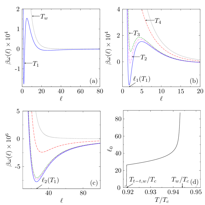
Figure 1: Effective interface potential for systems governed by short- and
long-ranged interactions as function of the thickness of
the liquid film at gas-liquid coexistence in the presence of ions for the case that the pure,
i.e., salt-free,
solvent exhibits a critical wetting transition (without being preceded by a thin-thick
transition).
The parameters used are K, (i.e.,
), ,
, , , and
C/cm2 (see main text).
The effective interface potential has two local minima (at (see
(a) and (b))
and
(see (c))
with ), one of the two being the global one at a given temperature
(see (a)).
They have the
same
depth
at (not apparently visible). For the film
thickness is the
global minimum and diverges continuously as (see
(c)). The global
minimum
as a function of temperature is plotted in (d). At the film thickness exhibits
a finite jump and subsequently diverges smoothly for .
Accordingly, the system undergoes a thin-thick wetting transition at , followed by a continuous one at .
Five different temperatures, , ,
,
and are displayed in (a), (b), and (c) (using a common color code) with . (Note the different scales of the axes.)
The film thickness is measured in units of such that is the volume of a solvent
particle. Densities are measured in units of .
The thin-thick wetting transition at two-phase
coexistence, which precedes a standard second-order wetting scenario, has been discussed in the
context of wetting
in electrolytes in Ref.
Denesyuk2004 for a model of an ionic solution close to a charged wall in which the
solvent-solvent and solvent-wall interactions are short-ranged only and the contribution of the
ions to
the effective interface potential is calculated by solving the full Poisson-Boltzmann equation
instead of the linearized one as in the present study (see Sec. II). The thin-thick
transition
in Ref. Denesyuk2004 occurs in a restricted region of the parameter space, provided
that the transition in the pure solvent is first order and that , i.e, for
large ionic strength.
In contrast, within the present
approach the combined presence of short- and long-ranged interactions is
taken into account. As discussed above for the case of a
pure
solvent with short- and long-ranged interactions, a thin-thick transition
will
precede a long-ranged critical
wetting transition only if the short-ranged interactions alone would give rise to a
first-order wetting
transition in the case that the long-ranged interactions were negligible Indekeu1999 ; Indekeu2000 . This is precisely the case we encounter in the present context for the electrolyte
solution when solvent-solvent and solvent-wall long-ranged interactions are taken into account: In
the absence of these long-ranged interactions the transition is first-order if
(see Subsec. II.2), such that jumps from to
(see Fig.
1). Once the long-ranged interactions are taken into
account they block the jump of to and limit this jump to one with a
finite value . Once has reached the value a further increase in
temperature leads to the unfolding of the standard wetting scenario under the aegis of long-ranged
interactions at . Therefore, the thin-thick
wetting transition is the remnant of the first-order wetting transition that would occur in
the
electrolyte solution if the long-ranged solvent-solvent and solvent-wall interactions were
negligible (see Subsec. II.2).
We briefly give the main points of the literature and of our results.
(I)
If in the pure solvent short-ranged interactions favor first-order wetting but
additional
long-ranged interactions produce second-order wetting, one finds a thin-thick transition followed
by the continuous wetting transition Indekeu1999 ; Indekeu2000 . We confirmed this behavior
for our model, which allows for the thin-thick transition only via the competition between
short- and long-ranged interactions.
(II)
A thin-thick transition can be observed in the pure solvent even if there are only
short-ranged Piasecki ; Indekeu ; Langie or only long-ranged Dietrich1985
interactions.
(III)
We have considered a solvent with short- and long-ranged interactions which exhibits
a
second-order wetting transition without being preceded by a thin-thick transition. Adding ions
renders such a short-ranged contribution to the effective interface potential that the resulting
effective short-ranged interactions favor first-order wetting. This leads to a thin-thick
transition
preceding the continuous long-range type wetting transition. This mechanism is analogous to the one
in (I).
(IV)
If the solvent with short- and long-ranged interactions undergoes a continuous wetting
transition, which is preceded by a thin-thick transition, adding ions decreases the
transition temperature of the latter and increases the jump in film thickness.
(V)
If the pure solvent is governed by short-ranged interactions only and exhibits a
first-order
wetting transition, adding ions can lead to a continuous wetting transition preceded by a thin-thick
transition, provided that .
(VI)
If the solvent is governed by short-ranged interactions only, adding ions renders a
first-order wetting transition for . Adding further long-ranged interactions, which
favor continuous wetting, renders a second-order wetting transition of the long-range type,
preceded by a thin-thick transition.
IV Conclusions and Summary
We have implemented an improvement over the approximation of step-like varying density profiles in
order to derive analytic
expressions for the effective interface potential of electrolyte solutions near
charged walls. This approach consists of performing a Taylor expansion up to second order of the
local part of the grand canonical density functional around piecewise constant density profiles of
the solvent and of the ions. The
resulting mean-field
expressions for the effective interface potential allow one to predict general trends for the
wetting behavior of electrolyte
solutions in terms of the relevant system parameters such as the ionic strength and the surface
charge
density.
The present analysis, which is valid in the case of low ion density , shows that in the case of
short-ranged
solvent-solvent and solvent-wall interactions
wetting transitions in the presence of
electrostatic interactions are typically first order. This result can be
explained in terms of the competition between the two characteristic length scales in the system,
i.e., the bulk correlation length in the wetting liquid phase and the Debye length .
If , which is typically the case for dilute electrolyte solutions away from
(bulk)
critical points, a wetting transition at two-phase coexistence will be always first order
irrespective of its order in the pure, i.e., salt-free, solvent.
First-order wetting transitions in electrolyte solutions with solvent
interactions being short-ranged only have been observed in
previous
studies, too Denesyuk2003 ; Denesyuk2004 ; Oleksy2009 ; Oleksy2010 ; Ibagon . It is the merit
of
the present analysis of the effective interface potential to provide a transparent rationale
for the pre-eminence of first-order wetting in electrolyte solutions in terms of competing length
scales.
Moreover, if in those systems in addition long-ranged
solvent-solvent and solvent-wall interactions, which favor a critical wetting transition,
are present,
our analysis reveals the possibility of a wetting scenario which actually corresponds to
a sequence of two wetting transitions:
first an electrostatically induced (i.e., ) discontinuous jump between two
finite wetting film
thicknesses which upon raising the
temperature is
followed by a
continuous divergence of the wetting film thickness (see Fig. 1).
Within the present approach, in the case of short-ranged interactions the analytic expressions for
the coefficients of the exponential terms in the effective interface
potential (Eq. (35)) are simple and the necessary
conditions for first- and second-order wetting can be translated explicitly into conditions for
the parameters of the interaction potentials. However, in the case of additional long-ranged
interactions extra parameters make such a kind of translation more difficult. Nevertheless,
by choosing a set of parameters for the
interaction potentials based on actual values for the Hamaker constant and the critical
temperature and by fulfilling corresponding necessary conditions for the occurrence of
second-order
wetting in the pure solvent (formulated in terms of the coefficients and
(Eqs. (56),
(80), and
(81))), we have been able to analyze
the effect of ions and of the surface charge density of the confining wall on the wetting
behavior. We have found that if the pure solvent exhibits a second-order wetting transition
governed asymptotically by long-ranged interactions, adding ions typically introduces a
thin-thick
transition which precedes the ultimate continuous wetting transition (see Fig.
1).
We have
been able to put the occurrence of such a thin-thick wetting transition at gas-liquid coexistence
into the context of the literature, which discusses such a transition as the result of the
interplay between short- and long-ranged interactions. Here the corresponding short-ranged effective
interactions relevant for that are provided by the ions.
Appendix A Double parabola approximation for the pure solvent
The double parabola approximation (DPA) has been widely used in the context of wetting
phenomena in order to obtain analytically tractable density functionals Meister1983 ; Lipowsky1984 ; Holyst1987 ; Gelfand1987 ; Jin1993 ; Iwamatsu1993 ; Parry2006 ; Wojtowicz2013 .
Within this approximations, the grand canonical functional for the pure solvent,
i.e., and (see Eq. (1)) is given by
(60)
with
(61)
where and are, respectively, the (temperature dependent) liquid and gas
bulk densities at coexistence, and is fixed later in order to render the bulk
correlation length. Upon construction, the DPA requires an underlying theory which provides
expressions for the bulk densities
and the curvature of the local free energy density at coexistence Meister1983 ; Lipowsky1984 ; Holyst1987 ; Gelfand1987 ; Jin1993 ; Iwamatsu1993 ; Parry2006 ; Wojtowicz2013 .
For brevity we shall refrain from indicating the temperature dependence in our notation.
Within this approach, for a given profile the assigned film thickness is
defined as
(62)
Minimization of the functional in
Eq. (60) leads to
(63)
with the boundary conditions
(64)
At two-phase coexistence (as for the pure solvent case, i.e., , in the
present model given by Eq. (2)) and Eq. (63) reduces to
(65)
Comparison with Eq. (15) leads to .
Equation (65) together with the boundary conditions in Eq. (64) yields
(66)
where
(67)
The comparison between Eqs. (22) and (66) shows that the
coefficients , , and there play the same role as the coefficients
, , and , respectively, here. At coexistence and for
in Eq. (29) one obtains
(68)
i.e., the relative difference between the coefficients of the profiles in Eq. (22)
and in
Eq. (66) is exponentially small for film thicknesses
large compared to the
bulk correlation length.
Appendix B Bulk correlation length of the pure solvent
In the case of a bulk pure solvent (), the density functional
given by Eq. (1)
reduces to
(69)
If we consider a spatially uniform equilibrium state , the corresponding two-point correlation
function is obtained from , with
the inverse , where Evans . From Eq. (69) one obtains
(70)
The corresponding Fourier transform,
with dimensionless , is given by
(71)
where Eq. (16) has been used. , which is proportional
to the
static structure factor, can be written in the form
(72)
This allows one to identify with the bulk correlation
length.
For a discussion of the structure in the presence of ions (Eq. (1)) see Ref.
Bier2012 .
In a similar way for the case with long-ranged interaction between solvent particles (see Eq.
(47))
(73)
Therefore the bulk correlation length for this case is given by
(74)
with .
Appendix C First-order perturbation theory for including the long-ranged
interactions
The total grand canonical functional is given by
(75)
with given by Eq.
(1) whereas
is given by Eq. (48) and
depends only on . We choose a dimensionless coupling
parameter such that for the perturbation
is absent and for the
perturbation is fully present. The perturbed grand canonical functional is
(76)
where acts as an amplitude multiplying both and (see Eq. (48)). The equilibrium densities
and
minimize :
(77)
Furthermore, the equilibrium densities
and
which
minimize are known (see Sec. II).
In order to proceed we write the equilibrium densities and as power series in terms of ,
(78)
and perform a functional Taylor expansion of the grand canonical potential
around
, :
(79)
with and (see Eq. (78)). In Eq. (79) the first derivatives vanish
because and
minimize .
Hence up to second order in .
Appendix D Coefficients for the effective interface potential in the presence of
long-ranged
interactions
The effective interface potential for the model with long-ranged interaction
(Sec. III) is
calculated by following the procedure described in Sec. II. The double
integrals in Eq. (48) have been evaluated by performing an
asymptotic
expansion for .
The analytic expressions for the coefficients in Eq. (56) are given by (see Appendix
E)
(80)
and
(81)
The coefficients and can be compared with the general expressions obtained in Ref.
SDMN within a systematic study of wetting transitions of a simple one-component fluid,
inter alia including the
presence of van der Waals tails. There the effective interface potential is expressed in terms of
the interfacial profiles which
emerge as a consequence of wetting phenomena, i.e., the wall-liquid and the free liquid-gas
interface for wetting of the wall-gas interface. Within that approach the
effective interface potential at coexistence is given by
(82)
where
(83)
(84)
and
(85)
with
(86)
and
(87)
The coefficients , for the present model are given by Eqs. (51) and (52);
and are moments of the wall-liquid interface profile
and of the free liquid-gas interface profile , respectively:
(88)
and
(89)
The wall-liquid and the free liquid-gas interface profile can be calculated within our approach by
following a procedure analogous to the one described in Sec. II. To this end, in the case of
the
wall-liquid interface for the pure solvent, the Taylor expansion up to second order of the local
part of
the
functional in Eq. (1) with and , is performed about
for where is the Heaviside
function. This
leads to the wall-liquid density profile
(90)
Within the approximation discussed in Appendix C, this expression, obtained from
minimizing and shifting by , is inserting into the general expression in Eq.
(88) corresponding to and yields
(91)
As expected, Eq. (91) respects the expected property that in the sharp-kink limit
(i.e, vanishing interfacial width ) reduces to . With this result Eq.
(81) can be rewritten as
.
For the free
liquid-gas interface, we consider the functional in Eq. (69). All integrals
extend over a macroscopic volume. We impose the boundary conditions
and . Accordingly, the Taylor expansion up to second order of the
local part of the functional is
performed
about the sharp-kink profile
(92)
The resulting liquid-gas density profile based on is
(93)
Again, within the approximation discussed in Appendix C, this profile stemming from
is inserted into the general expression in Eq. (89), which is based on
, and renders
(94)
Inserting Eqs. (51), (52), (91), and (94) into Eqs. (83)
and (84) one obtains (with )
(95)
This leads to the satisfactory statement that if the general results in Ref. SDMN for the
effective interface potential are applied to the present model one finds the same effective
interface potential as the one obtained directly within the present model.
Appendix E Derivation of the effective interface potential for the model with
long-ranged interactions
The derivation of in Eq. (56) follows the same procedure as described in
Sec
II. We perform a Taylor expansion up to second order of the local part of the functional in Eq.
(47)
about the sharp-kink profile in Eq. (8) shifted by and the
sharp-kink profile in Eq. (9) with the bulk
state being determined by Eq. (98) below. From this
expansion
we obtain an approximate variational functional for the model with
long-ranged interactions. By subtracting the bulk contribution
of the gas phase we obtain the surface contribution to
this variational
functional:
(96)
where describes the excluded volume due to the repulsive part of the substrate potential
given by Eq. (46) and
(97)
The bulk grand canonical potential density per is given by
(98)
, , , and are abbreviations for the
following types of integrals:
(99)
(100)
(101)
and
(102)
The integrals in Eqs. (100)-(102) are evaluated at two-phase coexistence using the
solutions for obtained in Sec. II (see Eqs. (22) and
(29)).
We are interested in the asymptotic behavior of these integrals in the limit . Using
Eqs. (22) and (46), can be written as
(103)
Asymptotic approximations for the integrals in Eq. (103) are obtained via integrating by
parts repeatedly:
(104)
and
(105)
with
(106)
Here and in the following we have used the properties
and
for two polynomials and
of degrees
and with the leading coefficients and , respectively, of the
leading terms which follows from
L’Hôpital’s rule.
For convenience, we write the expressions in Eq. (29) as
(107)
with
(108)
Collecting only algebraic terms up to the order
, one obtains for
(109)
Analogously, for one has
(110)
In order to calculate integrals of the type we first integrate Eq. (97)
using the various
integration limits appearing in Eq. (96) so that
where we have changed the integration variable to . Asymptotic approximations for the
integrals in Eq. (114) are obtained via integrating by parts
repeatedly:
(115)
(116)
and
(117)
with
(118)
and
(119)
with
(120)
Additionally, for one has
(121)
Note that Eqs. (115) and (116) contain terms which increase exponentially
with .
However, these two integrals are multiplied by which decays exponentially with
(see Eqs. (103) and (107)).
Collecting constants and algebraic terms up to the order
, for one obtains
where we have changed the integration variable to . Using Eqs.
(115)-(121) one obtains asymptotically
(125)
Similarly, can be written as (see Eqs.
(22)
and (113))
(126)
where we have changed the integration variable to and , respectively.
Using Eqs.
(115)-(121), this leads to the asymptotic behavior
(127)
Integrals of the type can be written as (see Eqs.
(22) and Eqs. (97))
(128)
(129)
(130)
and
(131)
with .
The double integrals can be reduced to single ones as follows:
(132)
(133)
and
(134)
Inserting these expressions into Eqs. (128)-(130) leads to
(135)
(136)
and
(137)
We note the following relations:
(138)
Accordingly we obtain
(139)
In order to determine the asymptotic behavior of the integrals in Eqs. (135)-(137) we
repeatedly integrate by parts so that
(140)
(141)
with
(142)
and
(143)
Finally, collecting the leading terms for one obtains the asymptotic behavior
(144)
Inserting the results for these integrals (see Eqs.
(109), (110), (122), (123), (125), (127), and
(144)) into Eq. (96), one obtains the effective interface
potential given by Eq.
(56); the index refers to long-ranged interactions (Sec. III).
References
(1) N. A. Denesyuk and J.-P. Hansen, Europhys. Lett. 63, 261 (2003).
(2) N. A. Denesyuk and J.-P. Hansen, J. Chem. Phys. 121, 3613 (2004).
(3) A. Oleksy and J.-P. Hansen, Mol. Phys. 107, 2609 (2009).
(4) A. Oleksy and J.-P. Hansen, J. Chem. Phys. 132, 204702 (2010).
(5) I. Ibagon, M. Bier, and S. Dietrich, J. Chem. Phys. 138, 214703
(2013).
(6) R. Evans, Adv. Phys. 28, 143 (1979).
(7) M. Schick, in Liquids at interfaces, edited by J. Charvolin, J. F. Joanny, and J. Zinn-Justin (North-Holland, Amsterdam, 1988), p. 415.
(8) S. Dietrich, in Phase Transitions
and Critical Phenomena, edited by C. Domb and J. L. Lebowitz (Academic, London,
1988), Vol. 12, p. 1.
(9) M. Bier, A. Gambassi, and S. Dietrich, J. Chem. Phys. 137, 034504
(2012).
(10) M. Rubinstein and R. H. Colby, Polymer Physics (Oxford University
Press, 2004).
(11) J. W. Cahn and J. E. Hilliard, J. Chem. Phys. 28, 258
(1958).
(12) H. Nakanishi and M. Fisher, Phys. Rev. Lett. 49, 1565 (1982).
(13) C.J.F. Böttcher, Theory of Electric Polarization (Elsevier,
Amsterdam, 1973).
(14) L. Bocquet, E. Trizac, and M. Aubouy
J. Chem. Phys. 117, 8138 (2002).
(15) T. Aukrust and E. H. Hauge, Phys. Rev. Lett. 54, 1814 (1985).
(16) T. Getta and S. Dietrich, Phys. Rev. E 57, 655 (1998).
(17) J. N. Israelachvili, Intermolecular and surface forces,
2nd ed. (Academic Press, 1991).
(18) J. O. Indekeu, K. Ragil, D. Bonn, D. Broseta, and J. Meunier, J. Stat. Phys.
95, 1009 (1999).
(19) J. O. Indekeu, Phys. Rev. Lett. 85, 4188 (2000).
(20) J. Piasecki and E. H. Hauge, Physica A 143, 87 (1987).
(21) J. O. Indekeu, Europhys. Lett. 10, 165 (1989).
(22) G. Langie and J. O. Indekeu, J. Phys. Condens. Matter
3, 9797 (1991).
(23) S. Dietrich and M. Schick, Phys. Rev. B 31, 4718 (1985).
(24) N. Shahidzadeh, D. Bonn, K. Ragil, D. Broseta, and J. Meunier, Phys. Rev.
Lett. 80, 3992 (1998).
(25) D. E. Sullivan, Phys. Rev. B 20, 3991 (1979).
(26) S. Dietrich and M. Napiórkowski, Phys. Rev. A 43, 1861 (1991).
(27)
T. Meister and H. Müller-Krumbhaar,
Phys. Rev. Lett. 51, 1780 (1983).
(28)
R. Lipowsky,
Z. Phys. B 55, 345 (1984).
(29)
R. Hołyst and A. Poniewierski,
Phys. Rev. A 36, 5628 (1987).
(30)
M.P. Gelfand and R. Lipowsky,
Phys. Rev. B 36, 8725 (1987).
(31)
A.J. Jin and M.E. Fisher,
Phys. Rev. B 47, 7365 (1993).
(32)
M. Iwamatsu,
J. Phys.: Condens. Matter 5, 7537 (1993).
(33)
A.O. Parry, C. Rascón, N.R. Bernardino, and J.M. Romero-Enrique,
J. Phys.: Condens. Matter 18, 6433 (2006).
(34)
A. Wójtowicz and M. Napiórkowski,
J. Phys.: Condens. Matter 25, 485007 (2013).