Models of DNA denaturation dynamics: universal properties

Abstract

We briefly review some of the models used to describe DNA denaturation dynamics, focusing on the value of the dynamical exponent $z$, which governs the scaling of the characteristic time $\tau\sim L^{z}$ as a function of the sequence length $L$. The models contain different degrees of simplifications, in particular sometimes they do not include a description for helical entanglement: we discuss how this aspect influences the value of $z$, which ranges from $z=0$ to $z\approx 3.3$. Connections with experiments are also mentioned.

1 Introduction

Helical structures, also in a double helical form, are ubiquitous in nature. The most famous example is of course DNA. The main reason for which nature has selected a double helical form for the molecule which stores all genetic information is probably its stability [1]. In fact, the twisting of the strands around each other adds cohesion to the whole molecule because the geometrical entanglement helps the base pairing interactions to prevent thermal fluctuations from opening the DNA at random.

The entanglement of the two strands around each other is expected to have a strong influence on the denaturation dynamics, and in the characteristic times needed to separate the strands from one another. However, several models of DNA denaturation do not explicitly take helical degrees of freedom into account. In this paper we review some models of DNA denaturation dynamics, discussing their advantages and shortcomings. Our focus is the asymptotic scaling of the characteristic time of denaturation $\tau$ as the function of the sequence length, $L$, which is expected to behave asymptotically as

$$\tau\sim L^{z}$$

for lengths $L\gg\ell_{p}$, where $\ell_{p}$ is the persistence length. In the previous equation $z$ defines the dynamical exponent. As we will see, values found for $z$ in the literature are spread from $z=0$ up to $z=3.3$, depending mostly on whether the helical degrees of freedom are taken into account. It is natural to expect that the time necessary to disentangle a double helix scales with its length. In living cells a class of enzymes called topoisomerases [2] cut and rejoin portions of DNA to remove unwanted knots, linking, or excessive twist. In an in vitro system where topoisomerases are absent the two strands have to rotate around each other to loose their twist and separate from each other.

Here we consider a laboratory situation where double-stranded DNA is immersed in an environment that facilitates its denaturation, such as high temperature aqueous solution and/or suitable ionic conditions. Experiments showed that the fraction of molten DNA increases for increasing temperature [3]. Denaturation in this case is an entropy-driven process, as the energy that was crucial to bind the two DNA strands is overwhelmed by the entropic gain that the two strands achieve by moving away from each other. The passage from the initial ordered state to the final coil state goes through a sequence of intermediate states that should be understood.

To date there are several simplified models that try to capture the salient features of the DNA melting dynamics. The simplifications, in some cases very strong, are necessary to reduce the huge number of degrees of freedom of a long DNA duplex to a manageable one in simulations, or to have models that are simple enough to be treated analytically. However, sometimes the simplifications could be meaningful in a restricted context, and might be excessive for the problem considered. So far, experiments of denaturation dynamics [4] were restricted to short sequences (e.g. $\approx 20$ base pairs). Thus the determination of the dynamical exponent $z$ from experiments remains an open issue. In any case, in the following we present some arguments about the merits and shortcomings of some of the models proposed in the literature for describing the dynamics of DNA denaturation. The two classes of models we mainly consider are the Poland-Scheraga (PS) model [5, 6, 7] (or other simple directed models of polymers [8]) and three-dimensional simplified models of polymers [9, 10]. We also briefly discuss results obtained with the Peyrard-Bishop model [11, 12, 13].

2 Poland-Scheraga and related models

A state in the PS model [5] consists in a string of $L$ bits, either $0$ or $1$, and hence it is evidently a strong reduction of the DNA degrees of freedom, see Fig. 1. Each “$1$” represents a bound portion, which for us is conveniently identified with a full helical turn of $\approx 10$ base pairs, with an associated a Boltzmann weight $q=\exp[-\epsilon/k_{B}T]$. A purely entropic weight is associated to open bases, represented by $0$’s. Each string of $\ell$ consecutive $0$’s represents a DNA bubble of length $2\ell$ (each strand contributes with $\ell$ steps to one half of the bubble). Say that a configuration contains $m$ of such bubbles: each bubble $i\in[1,m]$ of length $2l_{i}$ carries an entropic weight

$$w_{i}\simeq As^{2\ell_{i}}\ell_{i}^{-c}$$

as derived from the equilibrium statistical mechanics of polymers [14]. Here $s$ is the “fugacity” per unit of length, while the factor $\ell_{i}^{-c}$ describes a universal power-law correction with $c\approx 2.14$ if self-avoidance between all polymer segments is taken into account [14, 15]. The constant $A$ in this case includes the cost of starting a bubble in the DNA. Thus the full weight of a configuration with $b$ bound pairs and $m$ bubbles is

$$W=q^{b}\times w_{1}\times w_{2}\times\cdots\times w_{m}$$

with the constraint $L=b+\ell_{1}+\ell_{2}+\ldots+\ell_{m}$.

Originally the model was developed for open linear DNA, without constraints on the number and dimension of bubbles. The picture is different if the twist between the two strands is conserved, as in a PS model of DNA loops [16], or if plectonemic structures storing helicity are included in the model [17]. These works show that the effect of helical constraints is relevant for thermodynamical properties. Let us now see what are the differences between dynamical properties of models with or without helices.

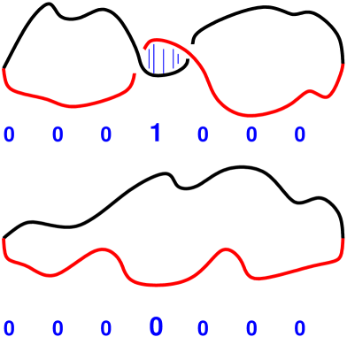
Figure 1: Sketch of PS configurations with $L=7$ sites: (top) “0001000” represents two bubbles separated by a helix; (bottom) a single bubble “0000000”. A “Glauber” move applied to the “1” of the first configuration would yield the second one, but it would imply a nonlocal rotation of either the left or the right bubble.

Consider two configurations $x$ and $y$ with equilibrium weights $W_{x}$ and $W_{y}$. In simulations, detailed balance in the dynamics is preserved if the rate $k(x\to y)$ for going from $x$ to $y$ and its reverse $k(y\to x)$ satisfy $W_{x}\,k(x\to y)=W_{y}\,k(y\to x)$. This can be achieved for example with a Metropolis acceptance rule. There are several choices of dynamics, depending on the updating rules for a given configuration. If one applies a Glauber-like scheme with local moves changing a $0$ into a $1$ or viceversa (an example is in Fig. 1), the denaturation time $\tau\sim 1$, i.e. $z=0$ [6]. But this dynamics does not take the entanglement of the two strands into account: after the breaking the bonds the two two strands still need to disentangle. Another possibility for the local updates is a Kawasaki-like strategy $01\leftrightarrow 10$ preserving the amount of entanglement (number of $1$’s) in the bulk [7]. Such helical entanglement is dissipated only at the boundaries (site $1$ and site $L$), which is the typical transition when the setup is such that the weights $q<s^{2}$. If this scheme is applied, starting with bound configurations from a low temperature regime, the denaturation time $\tau\sim L^{z}$ with $z\simeq 3$. Moreover, the scaling of the number of bubbles reveals a maximum for another intermediate timescale $\tau_{1}\sim L^{2.15}$. A possible explanation for the large $z\simeq 3$ value was also provided in [7]. The latter approach, trying to include entanglement effects due to the double-helical initial constraint, yields typical timescales that resemble those of another polymeric dynamics where entanglement is relevant, namely reptation of polymers in dense melts [18, 19].

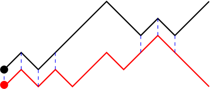
Figure 2: Sketch of the model proposed in [8]: two interacting directed walks on a tilted square lattice.

The shortcomings of the PS approach are its strong dependence on the choice of dynamical rules, the fact that by definition only configurations in the form paired-unpaired with respect to the DNA sequence are allowed, which is a rough coarse-grained representation of the actual configuration of the molecule during denaturation.

Besides the PS model, also models of directed polymers were proposed. They are simple enough that an analytical treatment is possible. An example is the model sketched in 2, proposed by Marenduzzo et al [8]. A pair of directed polymers starting from neighboring sites on a tilted square lattice are mutually avoiding and gain a unit of energy each time they are close to each other (dashed lines in the figure). One can also apply a force pulling away the two right extremities, but the case without force is what we are interested in here. Compared to the PS model, one can see that the bound segments have some entropy, since there are two directions for every step. Moreover, the entropy of the bubbles is not assumed. However, this model still misses the key ingredient of the helical degrees of freedom, and hence again its dynamics resembles more a polymer desorption than an unwinding. The exponent found for the case without forces (and with bubbles) was $z=4/3$.

3 Simulations of lattice and off-lattice polymers

The previous classes of models, although quite efficient to simulate and study, still contain some approximations. For instance, the three-dimensional entanglement of the two chains is neglected. Computer simulations of interacting self-avoiding polymers allow to study the dynamics of denaturations of chains of about $L\approx 10^{3}$ monomers without resorting to uncontrolled approximations. In these simulations, hydrodynamics effects are usually neglected and the polymer configurations are updated following a sequential local update using detailed balance dynamics. Particularly interesting are lattice polymers in which the updates consist in corner and end- flips, which can be very efficiently implemented and correspond to Rouse dynamics [20]. These types of simulations were recently employed to study several aspects of the denaturation dynamics [21], in the case of absence of bubbles and without winding of the two strands (the two polymer strands are paired as in a “zipper”). In this system the denaturation times scale with a dynamical exponent $z=1$, whereas renaturation dynamics is “anomalous” with $z\approx 1.4$, an exponent also found in simulations of translocation dynamics [22, 23].

The first study of disentanglement of double helical polymers dates back to Baumgärtner and Muthukumar [9] about thirty years ago. Despite generating the initial double helix with monomers on a cubic lattice, they then applied off-lattice corner flips. The steric constraint between monomer was preserved thus with repulsive potentials between them that was strong enough to prevent strand passages. The results they found included a large value $z\simeq 3.3$. These simulations were limited to relatively short chains, due to the limited computational power available at that time.

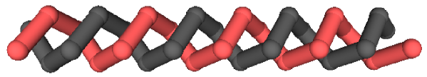
Figure 3: Double helical SAWs on the fcc lattice, with $N=16$ steps per strand, and $4$ sites per helical turn.

Recently a simulation of a self-avoiding walk (SAW) variant on the face-centered cubic (fcc) lattice yielded new results for long walks [10]. Again, starting from a double helical shape (see Fig 3) and letting the two walks to move via local rearrangements, it was monitored the minimal mutual distance $d$ between each of the monomers of one SAW from each of the monomers of the other SAW. Its square stays equal to the fcc lattice unit $d^{2}=2$ for a long time, until it starts to fluctuate to higher and higher values. The time when $d^{2}>10$ or $d^{2}>20$ for the first time, denoting the disentanglement of the chains, was used to define the denaturation time. Its average in both cases scales as $\tau\sim L^{2.57(3)}$, thus there is yet another candidate exponent $z=2.57$ for describing the disentangling process of two polymers prepared in a double-helical conformation.

The discrepancy between the more recent $z\simeq 2.57$ and previous $z\simeq 3.3$ is probably due to the difference in asymptoticity of the respective simulations. Since numerical results can be plagued by strong finite size effects, it is of course possible that $z\simeq 2.57$ is also not an asymptotic value yet. The equilibrium properties of winding angles in a system composed by a polymer attached to an end to an infinite straight rod are characterized by ratios of angles to logarithms of the chain length [24]. We are introducing these systems because a polymer wrapped as a helix around a bar can be considered a good surrogate of a double helical structure. The presence of $\log L$ in the statistics of this systems warns us that the simple power-law assumption $\tau\sim L^{z}$ might need some logarithmic corrections. This problem is currently under investigation [25].

4 Peyrard-Bishop model

Another classical model for describing DNA denaturation is the model introduced by Peyrard and Bishop in 1989 [11] and later improved by Dauxois, Peyrard, and Bishop (DPB) to add a non-linear coupling between adjacent base pairs [12]. In its original formulation a DNA configuration is described by a set of continuous variables $y_{i}\geq 0$ giving the distance between two base pairs along the sequence of length $N$ ($1\leq i\leq N$). The interaction between opposite bases is given by a short range Morse potential and there is usually also a stacking interaction between adjacent bases along the same strand. A further refined version of the DPB model with helical degrees of freedom was also studied [26, 27].

Many studies on the DPB model, in which specific types of dynamics were employed, focused so far on equilibrium quantities, as the fraction of open base pairs at a given temperature, or on dynamical aspects not directly related to denaturation times. A very recent study of the dynamics of the DPB model used the reactive flux method [13], a very powerful technique to deal with systems with very slow timescales. In particular, the denaturation rate above the melting temperature was investigated as a function of the sequence composition and length. The rate was found to behave non-monotonically as function of the sequence length and to be strongly influenced by the sequence composition. From the data available in Ref. [13] it is however not possible to extract a dynamical exponent, therefore the issue of the value of $z$ and of the relevance of helical degrees of freedom in the different versions of the DPB model is currently still open. Since the model describes bases regularly stacked, however, it would seem not correct to utilize it for describing the chaotic entanglement of denatureted DNA strands.

5 Conclusions

We have listed a variety of results concerning the scaling of DNA denaturation time with its chain length. Each of the results can tell us something about a particular aspect of DNA denaturation. In general, the inclusion of helical degrees of freedom and consequently of geometrical entanglement slows down the dynamics, giving rise to a higher exponent $z$.

We believe that the models of three-dimensional polymers are the most suitable for describing full denaturation of very long DNA immersed in a solvent above the denaturation temperature. In this sense it is a study of homopolymer dynamics, from an initial double helix representing the double stranded DNA to a final disentangled state of two polymers separated from each other. It would be interesting to measure experimentally such disentangling time. As an indicator of polymers separation one would need to consider some geometrical detectable aspect and not a measure of chemical bonds between strands, which can break in a timescale much faster than the disentangling one.

Acknowledgments

We acknowledge useful discussions with G. Barkema, M. Peyrard, F. Sattin, T. van Erp, J.-C. Walter, and with the participants of the workshop Inhomogeneous Random Systems (Paris, January 2012).

References

- [1] B. Alberts et al. (2002) Molecular Biology of the Cell, Gerland Science, New York.
- [2] F. B. Dean, A. Stasiak, T. Koller, and N. R. Cozzarelli (1985) J. Biol. Chem. 260, 4975.
- [3] R. M. Wartell and A. S. Benight (1985) Phys. Rep. 85, 67.
- [4] G. Altan-Bonnet, A. Libchaber, and O. Krichevsky (2003) Phys. Rev. Lett. 90, 138101.
- [5] D. Poland and H. Scheraga (1966) J. Chem. Phys. 45, 1464.
- [6] H. Kunz, R. Livi, and A. Süto (2007) J. Stat. Mech. P06004.
- [7] M. Baiesi and R. Livi (2009), J. Phys. A: Math. Theor. 42, 082003.
- [8] D. Marenduzzo, S. M. Bhattacharjee, A. Maritan, E. Orlandini, and F. Seno (2002) Phys. Rev. Lett. 88, 028102.
- [9] A. Baumgärtner and M. Muthukumar (1986) J. Chem. Phys. 84, 440.
- [10] M. Baiesi, G. Barkema, E. Carlon, and D. Panja (2010) J. Chem. Phys., 133, 154907.
- [11] M. Peyrard and A. R. Bishop (1989) Phys. Rev. Lett. 62, 2755.
- [12] T. Dauxois, M. Peyrard, and A.R. Bishop (1993) Phys. Rev. E, 47, R44. .
- [13] T. van Erp, and M. Peyrard (2012) Europhys. Lett. 98, 48004.
- [14] Y. Kafri, D. Mukamel, and L. Peliti (2000) Phys. Rev. Lett. 85, 4988.
- [15] M. Baiesi, E. Carlon, Y. Kafri, D. Mukamel, E. Orlandini, and A. L. Stella (2003) Phys. Rev. E 67, 021911.
- [16] J. Rudnick and R. Bruinsma (2002) Phys. Rev. E 65, 030902(R).
- [17] A. Kabakçıoğlu, A. Bar and D. Mukamel (2012) Phys. Rev. E 85, 051919.
- [18] E. Carlon, A. Drzewinski, and J. M. J. van Leeuwen (2001) Phys. Rev. E 64, 010801.
- [19] W. Paul, K. Binder, D. W. Heermann, and K. Kremer (1991) J. Chem. Phys. 95, 7726.
- [20] M. Doi and S. F. Edwards (1989) The Theory of Polymer Dynamics (Oxford University Press, New York)
- [21] A. Ferrantini and E. Carlon (2011) J. Stat. Mech.: Theory and Exp. 2011, P02020.
- [22] H. Vocks and D. Panja and G. T. Barkema and R. C. Ball (2008) J. Phys.: Condens. Matter 20, 095224.
- [23] K. Luo, T. Ala-Nissila, S.-C. Ying and R. Metzler (2009) Europhys. Lett. 88, 68006.
- [24] J.-C. Walter, G. Barkema, and E. Carlon (2011) J. Stat. Mech. P10020.
- [25] J.-C. Walter, M. Baiesi, G. Barkema, and E. Carlon (2012) in preparation.
- [26] M. Barbi, S. Cocco, and M. Peyrard (1999) Phys. Lett. A 253, 358.
- [27] M. Barbi, S. Lepri, M. Peyrard, and N. Theodorakopoulos (2003) Phys. Rev. E 68, 061909.