Implications of uniformly distributed, empirically informed priors for phylogeographical model selection: A reply to Hickerson et al.

Abstract

Establishing that a set of population-splitting events occurred at the same time can be a potentially persuasive argument that a common process affected the populations. Recently, Oaks et al. (2013) assessed the ability of an approximate-Bayesian model-choice method (msBayes) to estimate such a pattern of simultaneous divergence across taxa, to which Hickerson et al. (2014) responded. Both papers agree that the primary inference enabled by the method is very sensitive to prior assumptions and often erroneously supports shared divergences across taxa when prior uncertainty about divergence times is represented by a uniform distribution. However, the papers differ about the best explanation and solution for this problem. Oaks et al. (2013) suggested the method’s behavior was caused by the strong weight of uniformly distributed priors on divergence times leading to smaller marginal likelihoods (and thus smaller posterior probabilities) of models with more divergence-time parameters (Hypothesis 1); they proposed alternative prior probability distributions to avoid such strongly weighted posteriors. Hickerson et al. (2014) suggested numerical approximation error causes msBayes analyses to be biased toward models of clustered divergences because the method’s rejection algorithm is unable to adequately sample the parameter space of richer models within reasonable computational limits when using broad uniform priors on divergence times (Hypothesis 2). As a potential solution, they proposed a model-averaging approach that uses narrow, empirically informed uniform priors. Here, we use analyses of simulated and empirical data to demonstrate that the approach of Hickerson et al. (2014) does not mitigate the method’s tendency to erroneously support models of highly clustered divergences, and is dangerous in the sense that the empirically-derived uniform priors often exclude from consideration the true values of the divergence-time parameters. Our results also show that the tendency of msBayes analyses to support models of shared divergences is primarily due to Hypothesis 1, whereas Hypothesis 2 is an untenable explanation for the bias. Overall, this series of papers demonstrate that if our prior assumptions place too much weight in unlikely regions of parameter space such that the exact posterior supports the wrong model of evolutionary history, no amount of computation can rescue our inference. Fortunately, as predicted by fundamental principles of Bayesian model choice, more flexible distributions that accommodate prior uncertainty about parameters without placing excessive weight in vast regions of parameter space with low likelihood increase the method’s robustness and power to detect temporal variation in divergences.

1 Introduction

Biogeographers frequently seek to explain population and species differentiation on geographical phenomena. Establishing that a set of population-splitting events occurred at the same time can be a potentially persuasive argument that a set of taxa were affected by the same geographic events. The approximate-Bayesian method, msBayes, allows biogeographers to estimate the probabilities of models in which multiple sets of taxa diverge at the same time (Hickerson et al., 2006; Huang et al., 2011).

Recently, Oaks et al. (2013) used this model-choice framework to study 22 pairs of vertebrate lineages distributed across the Philippines; they also studied the behavior of the msBayes approach using computer simulations. They found the method is very sensitive to prior assumptions and often supports shared divergences across taxa that diverged randomly over broad time periods, to which Hickerson et al. (2014) responded. Oaks et al. (2013) and Hickerson et al. (2014) agree on the fundamental methodological point about the model selection performed in msBayes:

• Representing prior uncertainty about divergence-time parameters with a uniform distribution can lead to spurious support for models with few divergence events shared across taxa. Thus, the primary inference enabled by the approach is very sensitive to the priors on divergence times.

However, the two papers suggest alternative mechanisms by which the priors on divergence times cause this behavior:

1. Strongly weighted marginal likelihoods (Oaks et al., 2013): The uniform priors on divergence times lead to very small marginal likelihoods (and thus smaller posterior probabilities) of models with many divergence-time parameters. The likelihood of these models is “averaged” over a much greater parameter space in which there is a large amount of prior weight and small probability of producing the data. (Jeffreys, 1939; Lindley, 1957).

2. Numerical-approximation error (Hickerson et al., 2014): Under broad uniform priors, the rejection algorithm implemented in msBayes is unable to adequately sample the space of the models within reasonable computational time, which leads to bias toward models with fewer divergence-time parameters because they are better sampled.

In Hypothesis 2, the problem is numerical-approximation error due to insufficient computation. In this scenario, given data from taxa that diverged randomly through time, the exact (true) posterior supports a model with many divergence-time parameters, but we are unable to accurately approximate this posterior. In Hypothesis 1, the problem is more fundamental; given data from taxa that diverged randomly through time, the exact posterior supports a model with simultaneous divergences across taxa. I.e., when accommodating prior uncertainty about divergence times with a uniform distribution, the exact posterior from Bayes’ rule leads us to the wrong conclusion about evolutionary history. Such posterior support for simultaneous divergence, even if “correct” from the perspective of Bayesian model choice, does not provide the biogeographical insights that a researcher who employs msBayes seeks to gain.

While these phenomena are not mutually exclusive, it is important to distinguish between them in order to determine how to improve our ability to estimate shared divergence histories. If Hypothesis 2 is correct, then the model is sound and we need to increase our computational effort or improve our Monte Carlo integration procedures. For example, Markov chain or sequential Monte Carlo algorithms might sample the posterior more efficiently than the simple Monte Carlo rejection sampler implemented in msBayes. Rather than alter the sampling algorithm, Hickerson et al. (2014) tried using narrow, empirically informed uniform priors in the hope that with less parameter space to sample, the rejection algorithm would produce better estimates of the posterior. Here, we discuss theoretical considerations for using empirically informed priors for Bayesian model choice and evaluate the approach of Hickerson et al. (2014) as a potential solution to the biases of msBayes. In their analyses, Hickerson et al. (2014) made an error by mixing different units of time, which invalidates the results presented in their response (see Supporting Information for details). We correct this error, but still find their approach will often support (1) clustered divergence models when divergences are random, and (2) models that exclude from consideration the true values of the parameters.

If Hypothesis 1 is correct, we need to correct the model, because no amount of computation will help; even if we could calculate the exact posterior, we would still reach the wrong interpretation about evolutionary history. Accordingly, Oaks (2014) has introduced a method that uses more flexible probability distributions (e.g., gamma) to accommodate prior uncertainty in divergence times without overly inhibiting the marginal likelihoods of models with more divergence-time parameters. This greatly increases the method’s robustness and power to detect temporal variation in divergences (Oaks, 2014). This is not surprising given the rich statistical literature showing that marginal likelihoods are very sensitive to the priors used in Bayesian model selection (e.g., Jeffreys, 1939; Lindley, 1957).

We also use analyses of simulated and empirical data to explore the distinct predictions made by Hypotheses 1 and 2. We show the behavior of msBayes matches the predictions of Hypothesis 1, but not Hypothesis 2. This strongly suggests that the method tends to support models of shared divergences not because of insufficient computation, but rather due to the larger marginal likelihoods of these models under the prior assumption of uniformly distributed divergence times.

2 The potential implications of empirical Bayesian model choice

Hickerson et al. (2014) suggest a very narrow, highly informed uniform prior on divergence times is necessary to avoid the method’s preference for models with few divergence-time parameters. Such an empirical Bayesian approach to model selection raises some theoretical and practical concerns, some of which were discussed by Oaks et al. (2013) (see the last paragraph of “Assessing prior sensitivity of msBayes” in Oaks et al. (2013)); we expand on this here.

2.1 Theoretical implications of empirical priors for Bayesian model choice

Bayesian inference is a method of inductive learning in which Bayes’ rule is used to update our beliefs about a model $M$ as new information becomes available. If we let $\boldsymbol{\Theta}$ represent the set of all possible parameter values for model $M$, we can define a prior distribution for all $\theta\in\boldsymbol{\Theta}$ such that $p(\theta\,|\,M)$ describes our belief that any given $\theta$ is the true value of the parameter. If we let $\mathcal{X}$ represent all possible datasets then we can define a sampling model for all $\theta\in\boldsymbol{\Theta}$ and $X\in\mathcal{X}$ such that $p(X|\theta,M)$ measures our belief that any dataset $X$ will be generated by any state $\theta$ of model $M$. After collecting a new dataset $X_{i}$, we can use Bayes’ rule to calculate the posterior distribution

$$p(\theta\,|\,X_{i},M)=\frac{p(X_{i}\,|\,\theta,M)p(\theta\,|\,M)}{p(X_{i}\,|\,M)},$$ (1)

as a measure of our beliefs after seeing the new information, where

$$p(X_{i}\,|\,M)=\int_{\theta}p(X_{i}\,|\,\theta,M)p(\theta\,|\,M)d\theta$$ (2)

is the marginal likelihood of the model.

This is an elegant method of updating our beliefs as data are accumulated. However, this all hinges on the fact that the prior ($p(\theta\,|\,M)$) is defined for all possible parameter values independently of the new data being analyzed. Any other datasets or external information can safely be used to inform our beliefs about $p(\theta\,|\,M)$. However, if the same data are used to both inform the prior and calculate the posterior, the prior becomes conditional on the data, and Bayes’ rule breaks down.

Thus, empirical Bayes methods have an uncertain theoretical basis and do not yield a valid posterior distribution from Bayes’ rule (e.g., empirical Bayesian estimates of the posterior are often too narrow, off-center, and incorrectly shaped; Morris, 1983; Laird and Louis, 1987; Carlin and Gelfand, 1990; Efron, 2013). This is not to say that empirical Bayesian approaches are not useful. Empirical Bayes is a well-studied branch of Bayesian statistics that has given rise to many methods for obtaining parameter estimates that often exhibit favorable frequentist properties. (Morris, 1983; Laird and Louis, 1987, 1989; Carlin and Gelfand, 1990; Hwang et al., 2009).

Although empirical Bayesian approaches can provide powerful methods for parameter estimation, a theoretical justification for empirical Bayesian approaches to model choice is questionable. In Bayesian model choice, the primary goal is not to estimate parameters, but to estimate the probabilities of candidate models. In a simple example with two candidate models, $M_{1}$ and $M_{2}$, we can use Bayes’ rule to calculate the posterior probability of $M_{1}$ as

$$p(M_{1}\,|\,X_{i})=\frac{p(X_{i}\,|\,M_{1})p(M_{1})}{p(X_{i}\,|\,M_{1})p(M_{1})+p(X_{i}\,|\,M_{2})p(M_{2})}.$$ (3)

By comparing Equations 1 and 3, we see fundamental differences between Bayesian parameter estimation and model choice.

In Equation 1, we see that the posterior density of any state $\theta$ of the model, is the prior density updated by the probability of the data given $\theta$ (the likelihood of $\theta$). The marginal likelihood of the model only appears as a normalizing constant in the denominator. Thus, as long as the prior distribution contains the values of $\theta$ under which the data are probable and the data are strongly informative relative to the prior, the values of the parameters that maximize the posterior distribution will be relatively robust to prior choice, even if the posterior is technically incorrect due to using the data to inform the priors. However, if we look at Equation 3, we see that in Bayesian model choice it is now the marginal likelihood of a model that updates the prior to yield the model’s posterior probability. The integral over the entire parameter space of the likelihood weighted by the prior density is no longer a normalizing constant, rather it is how the data inform the posterior probability of the model. Because the prior probability distributions placed on the model’s parameters have a strong affect on the integrated, or “average”, likelihood of a model, Bayesian model choice tends to be much more sensitive to priors than parameter estimation (Jeffreys, 1939; Lindley, 1957). Another important difference of Bayesian model choice illustrated by Equation 3 is that the value of interest, the posterior probability of a model, is not a function of $\theta$ because the parameters are integrated out of the marginal likelihoods of the candidate models. Thus, unlike parameter estimates, the estimated posterior probability of a model is a single value (rather than a distribution) lacking a measure of posterior uncertainty.

The justification for an empirical Bayesian approach to parameter estimation is that giving the data more weight relative to the prior (i.e., using the data twice) will often shift the peak of the estimated distribution nearer to the true value(s) of the model’s parameter(s). However, there is no such justification for model selection, because unlike model parameters, the posterior probabilities of candidate models often have no clear true values. Model posterior probabilities are inherently measures of our belief in the models after our prior beliefs are updated by the data being analyzed. This complicates the meaning of model posterior probabilities when Bayes’ rule is violated by informing priors with the same data to be analyzed. By using the data twice, we fail to account for prior uncertainty and mislead our posterior beliefs in the models being compared; we will be over confident in some models and under confident in others.

Nonetheless, empirical Bayesian model choice does perform well for some problems. Particularly, in cases where large aggregate data sets are used for many parallel model-choice problems, pooling information to inform priors can lead to favorable group-wise frequentist coverage across tests (Efron, 2008). However, this is far removed from the single model-choice problem of msBayes. In the Supporting Information we use a simple example to help highlight the distinctions between Bayesian parameter estimation and model choice.

2.2 Practical concerns about empirically informed uniform priors for Bayesian model choice

In addition to the theoretical concerns discussed above, there are practical problems with using narrow, empirically informed, uniform priors. The results of Hickerson et al.’s (2014) reanalysis of the Philippine dataset strongly favored models with the narrowest, empirically informed prior on divergence times, and thus their model-averaged posterior estimates are dominated by models $M_{1}$ and $M_{2}$ (see Table 1 of Hickerson et al. (2014)). This is concerning, because the narrowest $\tau$ prior used by Hickerson et al. (2014) ($\tau\sim U(0,0.1)$) likely excludes the true divergence times for at least some of the Philippine taxa. Hickerson et al. (2014) set this prior to match the 95% highest posterior density (HPD) interval for the mean divergence time estimated under one of the priors used by Oaks et al. (2013) (see Tables 2 and 3 of Oaks et al. (2013)). Given this interval estimate is for the mean divergence time across all 22 taxa, it may be inappropriate to set this as the limit on the prior, because some of the taxon pairs are expected to have diverged at times older than the upper limit. Furthermore, this prior is excluded from the 95% HPD interval estimates of the mean divergence time under the other two priors explored by Oaks et al. (2013) (under these priors the 95% HPD is approximately 0.3–0.6; see Table 6 of Oaks et al. (2013)).

The strong preference for the narrowest prior on divergence times suggests the approach of Hickerson et al. (2014) is biased toward models with less parameter space and, as a consequence, will estimate model-averaged posteriors dominated by models that exclude true values of the parameters. We explored this possibility in two ways. First, we re-analyzed the Philippines dataset using the model-averaging approach of Hickerson et al. (2014), but set one of the prior models with a uniform prior on divergence times that is unrealistically narrow and almost certainly excludes most, if not all, of the true divergence times of the 22 taxon pairs. If small likelihoods of large models cause the method to prefer models with less parameter space (Hypothesis 1), we expect msBayes will preferentially sample from this erroneous prior yielding a posterior that is misleading (i.e., the model-averaged posterior will be dominated by a model that excludes the truth). Second, we generated simulated datasets for which the divergence times are drawn from an exponential distribution and applied the approach of Hickerson et al. (2014) to each of them to see how often the method excludes the truth.

2.2.1 Re-analyses of the Philippines dataset using empirical Bayesian model averaging

For our re-analyses of the Philippines dataset we followed the model-averaging approach of Hickerson et al. (2014), but with a reduced set of prior models to avoid their error of mixing units of time (see SI for details). We used five prior models, all of which had priors on population sizes of $\theta_{D}\sim U(0.0001,0.1)$ and $\theta_{A}\sim U(0.0001,0.05)$. Following Hickerson et al. (2014), each of these models had the following priors on divergence times: $M_{1}$, $\tau\sim U(0,0.1)$; $M_{2}$, $\tau\sim U(0,1)$; $M_{3}$, $\tau\sim U(0,5)$; $M_{4}$, $\tau\sim U(0,10)$; and $M_{5}$, $\tau\sim U(0,20)$. We simulated $1\times 10^{6}$ random samples from each of the models for a total of $5\times 10^{6}$ prior samples. For each model, we retained the 10,000 samples with the smallest Euclidean distance from the observed summary statistics after standardizing the statistics using the prior means and standard deviations of the given model. From the remaining 50,000 samples, we then retained the 10,000 samples with the smallest Euclidean distance from the observed summary statistics, this time standardizing the statistics using the prior means and standard deviations across all five models. We then repeated this analysis twice, replacing the $M_{1}$ model with $M_{1A}$ and $M_{1B}$, which differ only by having priors on divergence times of $\tau\sim U(0,0.01)$ and $\tau\sim U(0,0.001)$, respectively. While we suspect the prior of $\tau\sim U(0,0.1)$ used by Hickerson et al. (2014) likely excludes the true divergence times of at least some of the 22 taxa, we are nearly certain that these narrower priors exclude most, if not all, of the divergence times of the Philippine taxa.

Our results show that the model-averaging approach of Hickerson et al. (2014) strongly prefers the prior model with the narrowest distribution on divergence times across all three of our analyses, even when this model excludes the true divergence times of the Philippine taxa (Table 1). Given that the same number of simuations were sampled from each prior model, this behavior is not clearly predicted by insufficient computation (Hypothesis 2), but is a straightforward prediction of Hypothesis 1.

Hickerson et al. (2014) vetted the priors used in their model-averaging approach via “graphical checks,” in which the summary statistics from 1000 random samples of each prior model are plotted along the first two orthogonal axes of a principle component analysis (see Figure 1 of Hickerson et al. (2014)). To determine if such prior-predictive analyses would indicate the $M_{1A}$ and $M_{1B}$ models are problematic, we performed these graphical checks on our prior models. Unfortunately, these prior-predictive checks provide no warning that these priors are too narrow (Figure S3). Rather, the graphs suggest these invalid priors are “better fit” (Figure S3A–C) than the valid priors used by Oaks et al. (2013) (Figure S3D–F).

2.2.2 Simulation-based assessment of Hickerson et al.’s (2014) model averaging over empirical priors

To better quantify the propensity of Hickerson et al.’s (2014) approach to exclude the truth, we simulated 1000 datasets in which the divergence times for the 22-population pairs are drawn randomly from an exponential distribution with a mean of 0.5 ($\tau\sim Exp(2)$). All other parameters were identically distributed as the $M_{1}$–$M_{5}$ models (Table 1). We then repeated the model-averaging analysis described above, retaining 1000 posterior samples for each of the 1000 simulated datasets. For each simulation replicate, we estimated the Bayes factor in favor of excluding the truth as the ratio of the posterior to prior odds of excluding the true value of at least one parameter. Whenever the Bayes factor preferred a model excluding the truth, we counted the number of the 22 true divergence times that were excluded by the preferred model.

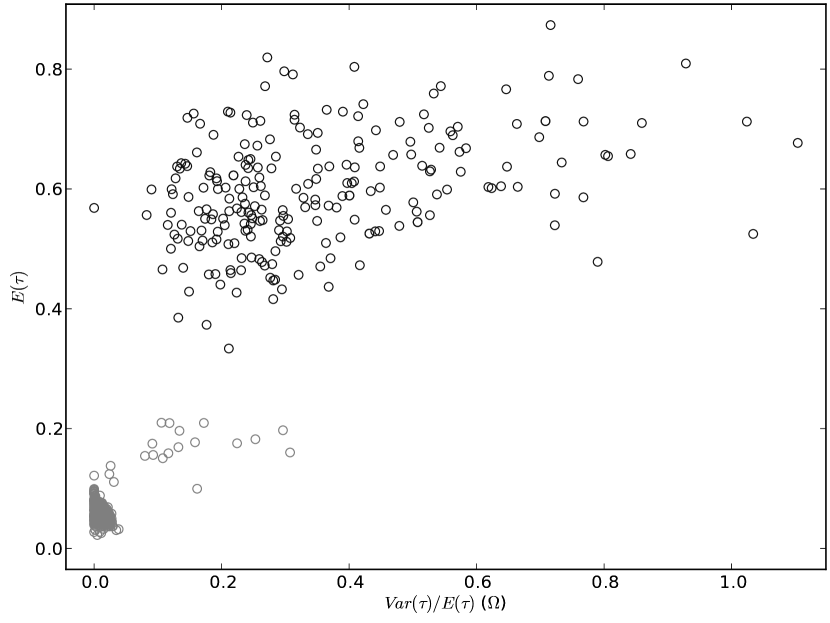
Figure 2: The joint posterior of the mean ($E(\tau)$) and dispersion index ($\Omega=Var(\tau{})/E(\tau)$) of divergence times for 22 vertebrate taxon pairs as estimated by Hickerson et al. (2014) (see Figure 2B of Hickerson et al. (2014)). The posterior samples are color-coded to indicate the erroneous mixture of timescales in the analysis of Hickerson et al. (2014); grey = $0.05/\mu$ generations and black = $0.02/\mu$ generations.

Our results show that the model-averaging approach of Hickerson et al. (2014) favors a model that excludes the true values of parameters in 97% of the replicates (90% with GLM-regression adjustment), excluding up to 21 of the 22 true divergence times (Figure 1). Importantly, the posterior probability of excluding at least one true parameter value is very high in most replicates (Figure 2). Using a Bayes factor of greater than 10 as a criterion for strong support, 66% of the replicates (87% with GLM-regression adjustment) strongly support the exclusion of true values (Figure 2).

The results of the above empirical and simulation analyses clearly demonstrate the risk of using narrow, empirically guided uniform priors in a Bayesian model-averaging framework. The consequence of this approach is obtaining a model-averaged posterior estimate that is heavily weighted toward models that exclude true values of the parameters. This is not a general critique of Bayesian model averaging. Rather, model averaging can provide an elegant way of incorporating model uncertainty in Bayesian inference. However, as predicted by Hypothesis 1, when averaging over models with narrow and broad uniform priors on a parameter that is not expected to have a uniformly distributed likelihood density, the posterior can be dominated by models that exclude from consideration the true values of parameters due to their larger marginal likelihoods (these models integrate over less space with high prior weight and low likelihood).

When using uniformly distributed priors, the alternative to capturing prior uncertainty is to risk excluding the true values one seeks to estimate. Fortunately, more flexible continuous distributions that are better suited as priors for the positive real-valued parameters of the msBayes model have been shown to greatly reduce spurious support for clustered divergence models while allowing prior uncertainty to be accommodated (Oaks, 2014).

3 Assessing the power of the model-averaging approach of Hickerson et al. (2014)

While our results above clearly demonstrate the risks inherent to the empirical Bayesian model-choice approach used by Hickerson et al. (2014), one could justify such risk if the approach does indeed increase power to detect temporal variation in divergences. We assess this possibility using simulations. Following Oaks et al. (2013), we simulated 1000 datasets with $\tau$ for each of the 22 population pairs randomly drawn from a uniform distribution, $U(0,\tau_{max})$, where $\tau_{max}$ was set to: 0.2, 0.4, 0.6, 0.8, 1.0, and 2.0, in $4N_{C}$ generations. All other parameters were identically distributed as the prior models. As above, we generated $5\times 10^{6}$ samples from prior models $M_{1}$–$M_{5}$ (Table 1). For each of the 6000 simulated datasets, we approximated the posterior by retaining 1000 samples from the prior.

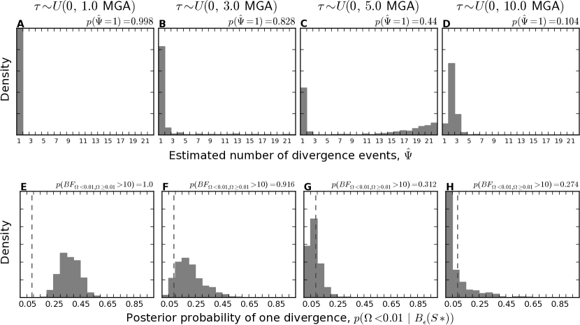
Figure 3: The tendency of the empirically informed model-averaging approach of Hickerson et al. (2014) to (A–D) infer clustered divergences and (E–H) support the extreme model of one divergence when applied to simulated datasets in which the divergence times of 22 pairs of populations are randomly drawn from the uniform distributions $\tau\sim U(0,\tau_{max})$ indicated at the top of each column of plots (divergence-time distributions are given in units of millions of generations ago (MGA) assuming a per-site rate of 1$\times 10^{-8}$ mutations per generation). Four of the six $\tau_{max}$ we simulated are provided; please see Figure S5 for a summary of all of the results.

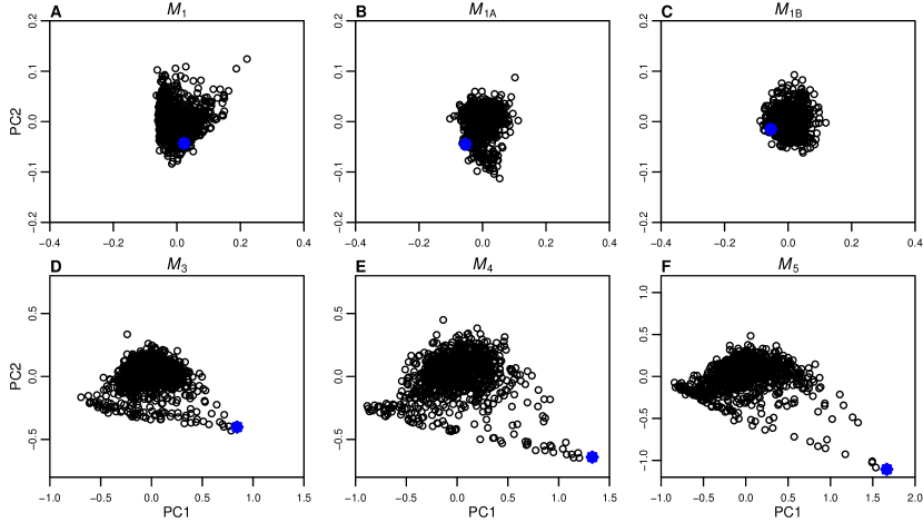
Figure 3: The prior predictive graphical checks recommended by Hickerson et al. (2014) for six prior models: (A) $M_{1}$ ($\tau\sim U(0,0.1)$), (B) $M_{1A}$ ($\tau\sim U(0,0.01)$), (C) $M_{1B}$ ($\tau\sim U(0,0.001)$), (D) $M_{3}$ ($\tau\sim U(0,5)$), (E) $M_{4}$ ($\tau\sim U(0,10)$), and (F) $M_{5}$ ($\tau\sim U(0,20)$). The three models that likely exclude true values of some divergence times of the 22 pairs of Philippine taxa (A–C) appear to have a “better fit” than the valid priors that likely cover the true divergence times (D–F). The plots project the summary statistics from 1000 random samples from each model onto the first two orthogonal axes of a principle component analysis, with the blue dot representing the observed summary statistics from the 22 population pairs of Philippine vertebrates.

Our results demonstrate that the approach of Hickerson et al. (2014) consistently infers highly clustered divergences across all the $\tau_{max}$ we simulated (Figure 3A–D & S5A–F). The approach often strongly supports (Bayes factor of greater than 10) the extreme case of one divergence event across all our simulation conditions (Figure 3E–H & S5G–L). The method also struggles to estimate the variance of divergence times ($\Omega$), whether evaluating the unadjusted (Figure S4A–F) or GLM-adjusted (Figure S4G–L) posterior estimates. Overall, the empirical Bayesian model-averaging approach leads to erroneous support for highly clustered divergences when populations diverged randomly over the last $8N_{C}$ generations. For loci with per-site rates of mutation on the order of $1\times 10^{-8}$ and $1\times 10^{-9}$ per generation, this translates to 10 million and 100 million generations, respectively.

Also, the results of our power analyses further demonstrate the propensity of Hickerson et al.’s (2014) approach to exclude true parameter values. Across all but one of the $\tau_{max}$ we simulated, the method favors a model that excludes the truth in a large proportion of replicates, and across many of the $\tau_{max}$ the preferred model will exclude a large proportion of the true divergence times (Figure 4A–D & S6A–F). Importantly, the posterior probability of excluding at least one true divergence value is also quite high across many of the $\tau_{max}$ (Figure 4E–H & S6G–L).

4 The importance of power analyses to guide applications of msBayes

Hickerson et al. (2014) presented a power analysis of msBayes under a narrow uniform divergence-time prior of 0–1 coalescent units ago. They found that under these prior conditions msBayes can, assuming a per-site rate of $1.92\times 10^{-8}$ mutations per generation, detect multiple divergence events among 18 taxa when the true divergences were random over 150,000 generations or more. It is important that investigators perform such simulations to determine the method’s power for their dataset, and decide if msBayes has sufficient temporal resolution to address their hypotheses; in the case of the Philippines dataset, it did not. When doing so, it is important to consider what prior conditions are relevant to the empirical system. It is rare for there to be enough a priori information to be certain that all taxa diverged within the last 4$N_{C}$ generations (i.e., 0–1 coalescent units). Also, it seems unlikely that when such prior information is available that being able to detect more than one divergence event in the face of 18 divergences that were random over 150,000+ generations will provide much insight into the evolutionary history of the taxa.

Inferring more than one divergence time shared across all taxa does not confirm the method is working well when analyzing data generated under random temporal variation in divergences (e.g., an inference of two divergence events could be biogeographically interesting yet spurious). Thus, it is important that investigators not limit their assessment of the method’s power to only differentiating inferences of one event or more (i.e. $\Psi=1$ versus $\Psi>1$). Rather, looking at the distribution of estimates, as in Figure 3 and Oaks et al. (2013), provides much more information about the behavior of the method.

5 The causes of support for models of co-divergence

To determine how best to improve the behavior of msBayes, it is important to determine the mechanism by which broad uniform priors cause support for clustered models of divergence. It is well established that vague priors can be problematic in Bayesian model selection. Models that integrate over more parameter space characterized by low probability of producing the data and relatively high prior density will have smaller marginal likelihoods (Jeffreys, 1939; Lindley, 1957). Given the uniformly distributed priors on divergence times employed in msBayes, the likelihood of models with more divergence parameters will be “averaged” over much greater parameter space, all with equal prior weight, and much of it with small likelihood (Hypothesis 1). In light of this fundamental statistical issue, it is not surprising that the method tends to support simple models.

However, Hickerson et al. (2014) conclude that the bias is caused by numerical- approximation error due to insufficient computation (Hypothesis 2). They argue the widest of the three priors on divergence times used by Oaks et al. (2013) would infrequently produce random samples of parameter values with many independent population divergence times as recent as the estimated gene divergence times presented in Oaks et al. (2013). However, this sampling-probability argument is based on some questionable assumptions. Oaks et al.’s (2013) gene-tree estimates were intended to provide only a rough comparison of the gene divergence times across the 22 taxa and assumed an arbitrary strict per-site rate of $2\times 10^{-8}$ mutations per generation for all taxa. Furthermore, because the branch-length units of the gene trees are in millions of years whereas the divergence-time prior of msBayes is in generations, Hickerson et al. (2014) make the implicit assumption that all 22 Philippine taxa have a generation time of one year. More importantly, even if we assume (1) the arbitrary strict clock is correct, (2) gene divergence times were estimated without error, and (3) all 22 taxa have one-year generation times, Hickerson et al.’s (2014) argument actually demonstrates that the models used by Oaks et al. (2013) with narrower priors on divergence times are densely populated with samples with large numbers of divergence parameters with values younger than the estimated gene divergence estimates. Thus, if Hickerson et al. (2014) are correct, analyses under these narrow priors should be much less biased toward clustered models of divergence. However, the magnitude of the bias is very similar across all three priors explored by Oaks et al. (2013). Hickerson et al. (2014) point out a case where the narrowest prior performs slightly better (panel L of Figures S32, S37, and S38 of Oaks et al. (2013)). However, it is important to note that these results suffered from a bug in msBayes, and after Oaks et al. (2013) corrected the bug, there are many cases where the narrowest prior performs slightly worse (see panels D–J of Figures 3 and S12 of Oaks et al. (2013)).

To disentangle whether Hypothesis 1 or 2 is the primary cause of the method’s erroneous support for simple models, we must look at the different predictions made by these two phenomena. For example, numerical error due to insufficient prior sampling (Hypothesis 2) should create large variance among posterior estimates and cause analyses to be highly sensitive to the number of samples drawn from the prior. Furthermore, if insufficient prior sampling is biasing estimates toward models with less parameter space we expect to see support for these models decrease as sampling from the prior increases. Oaks et al. (2013) did not see such sensitivity when they compared prior sample sizes of $2\times 10^{6}$, $5\times 10^{6}$, and $10^{7}$.

To explore this prediction further, we repeat the analysis of the Philippines dataset under the intermediate prior used by Oaks et al. (2013) ($\tau\sim U(0,10)$, $\theta_{D}\sim(0.0005,0.04)$, $\theta_{A}\sim(0.0005,0.02)$), using a very large prior sample size of $10^{8}$. When we look at the trace of the estimates of the dispersion index of divergence times ($\Omega$) as the prior samples accumulate (Figure S7) we do not see the trend predicted by Hypothesis 2. While approximation error is always present in any numerical analysis, it does not appear to be playing a large role in the biases revealed by the results of Oaks et al. (2013) or presented above.

A straightforward prediction if strongly weighted marginal likelihoods are causing the preference for simple models (Hypothesis 1) is that the bias should disappear as the model generating the data converges to the prior. Oaks et al. (2013) tested this prediction by performing 100,000 simulations to assess the model-choice behavior of msBayes when the prior model is correct. The results confirm the prediction of Hypothesis 1: msBayes estimates the probability of the one-divergence model quite well (or even underestimates it) when the prior is correct (see Figure 4 of Oaks et al. (2013)). We confirmed this same behavior for the model-averaging approach used by Hickerson et al. (2014) (see SI text and Figure S8). These results are not clearly predicted if insufficient computation was causing numerical error (Hypothesis 2). Even when the prior is correct, due to the discrete uniform prior on the number of divergence events ($\Psi$) implemented in msBayes, models with larger numbers of divergence-time parameters (and thus greater parameter space) will still be far less densely sampled than those with fewer divergence events (Oaks et al., 2013). Thus, the results of the simulations of Oaks et al. (2013) are more consistent with the fundamental sensitivity of marginal likelihoods to priors (Hypothesis 1).

This is further demonstrated by the results presented herein that show the model-averaging approach of Hickerson et al. (2014) prefers models with narrower $\tau$ priors (Table 1 and Figs. 1, 2 and 4) and fewer $\tau$ parameters (Figure 3). For these model-averaging analyses, insufficient prior sampling (Hypothesis 2) is an untenable explanation for the erroneous support for models with less parameter space, because (1) all of the prior models share the same dimensionality, and (2) the same number of random samples were drawn from each of the prior models. However, these results are predicted by Hypothesis 1, because the marginal likelihoods will be higher for models with narrower priors on divergence times and fewer divergence-time dimensions (these models integrate over less space with large prior weight and small likelihood).

6 Improving inference of shared divergences

In theory, the model-averaging approach of Hickerson et al. (2014) is appealing. It leverages a great strength of Bayesian statistical procedures, namely the ability to obtain marginalized estimates that incorporate uncertainty in nuisance parameters. However, when sampling over models with narrow-empirical and diffuse uniform priors for a parameter that is expected to have a very non-uniform likelihood density, models that exclude the true values of the parameters we aim to estimate will often have the largest marginal likelihoods.

The recommendations of Oaks et al. (2013) for mitigating the lack of robustness of msBayes are similar to those of Hickerson et al. (2014), but avoid the need for imposing an additional dimension of model choice and using priors that often exclude the truth. Oaks et al. (2013) suggest that uniform priors may not be ideal for many parameters of the msBayes model, and recommend the use of probability distributions from the exponential family. If we look at the prior distribution on divergence times imposed by the model-averaging approach of Hickerson et al. (2014) we see it is a mixture of overlapping uniforms with lower limits of zero (Figure S10). This looks very much like an exponential distribution, except that in any state of the model, all the divergence times are restricted to the hard bounds of one of the uniform distributions. Thus, it seems more appropriate to simply place a gamma prior (the exponential being a special case) on divergence times. This would capture the prior uncertainty that Hickerson et al. (2014) are suggesting for divergence times (Figure S10) while avoiding costly model-averaging and the constraint that all divergence times must fall within the hard bounds of the current model state. It also would allow an investigator to place the majority of the prior density in regions of parameter space they believe, a priori, are most plausible, but still capture uncertainty in the tails of distributions with low density. Indeed, Oaks (2014) has shown that the use of gamma distributions in place of uniform priors improves the power of the method to detect temporal variation in divergences and reduces erroneous support for clustered divergences.

7 Conclusions

We demonstrate how the approximate-Bayesian model-choice method implemented in msBayes can spuriously support models with less parameter space. This is caused by the use of uniform priors on divergence times. Uniform distributions necessitate the use of priors that place high density in unlikely regions of parameter space, less the risk of excluding the true divergence times a priori. These broad uniform priors reduce the marginal likelihoods of models with more divergence-time parameters. We show that the empirical Bayesian model-averaging approach of Hickerson et al. (2014) does not mitigate this bias, but rather causes it to manifest by sampling predominantly from models that often exclude the true values of the divergence times. Our results show that it is difficult to choose an uniformly distributed prior on divergence times that is broad enough to confidently contain the true values of parameters while being narrow enough to avoid strongly weighted and misleading posterior support for models with less parameter space. More generally, it is important to carefully choose prior assumptions about parameters in Bayesian model selection, because they can strongly influence the posterior probabilities of the models we seek to compare. No amount of computation can rescue our inference if our prior assumptions place too much weight in unlikely regions of parameter space such that the exact posterior supports the wrong model of evolutionary history.

The common inference of temporally clustered historical events (Barber and Klicka, 2010; Bell et al., 2012; Carnaval et al., 2009; Chan et al., 2011, 2014; Daza et al., 2010; Hickerson et al., 2006; Huang et al., 2011; Lawson, 2010; Leaché et al., 2007; Plouviez et al., 2009; Stone et al., 2012; Voje et al., 2009), when not accompanied with the necessary analyses to assess the robustness and temporal resolution of such results, should be treated with caution, because msBayes has been shown to erroneously infer clustered events over a range of prior conditions. Fortunately, Oaks (2014) has shown that alternative probability distributions allow prior uncertainty to be accommodated while avoiding excessive prior density in regions of low likelihood, which greatly improves inference of shared divergence histories.

The work presented herein follows the principles of Open Notebook Science. All aspects of the work were recorded in real-time via version-control software and are publicly available at https://github.com/joaks1/msbayes-experiments. All information necessary to reproduce our results is provided there.

8 Acknowledgments

We thank Melissa Callahan, Jake Esselstyn, Cameron Siler, Mark Holder, Rafe Brown, Emily McTavish, Daniel Money, Jordan Koch, Adam Leaché, Vladimir Minin, Luke Harmon, and three anonymous reviewers for insightful comments that greatly improved this work. We thank Michael Hickerson and co-authors for generously providing their data. J. Oaks and C. Linkem thank the National Science Foundation for supporting this work (DEB 1011423, DBI 1308885 and BIO-1202754). J. Oaks was also supported by the University of Kansas (KU) Office of Graduate Studies, Society of Systematic Biologists, Sigma Xi Scientific Research Society, KU Department of Ecology and Evolutionary Biology, and the KU Biodiversity Institute. We also thank Mark Holder, the KU Information and Telecommunication Technology Center, KU Computing Center, and the iPlant Collaborative for the computational support necessary to conduct the analyses presented herein.

fig0cm2.2cm fig

Table 1: Results of the model-averaging approach of Hickerson et al. (2014) applied to the Philippines dataset of Oaks et al. (2013) using three sets of prior models. All models used priors on population size of $\theta_{D}\sim U(0.0001,0.1)$ and $\theta_{A}\sim U(0.0001,0.05)$, and differ only in their prior on divergence-time ($\tau$) parameters. Each set of five models differ only in the divergence-time prior used for the model with the narrowest prior: $M_{1}$ ($\tau\sim U(0,0.1)$), $M_{1A}$ ($\tau\sim U(0,0.01)$), or $M_{1B}$ ($\tau\sim U(0,0.001)$). The approximate posterior probability of each model ($p(M_{i}\,|\,B_{\epsilon}(\mathbf{S}^{*}))$) is given for each of the three analyses. The posterior estimates are based on 10,000 samples retained from $1\times 10^{6}$ prior samples from each model.

		$p(M_{i}\,|\,B_{\epsilon}(\mathbf{S}^{*}))$
Model	$\tau$ prior	$M_{*}=M_{1}$	$M_{*}=M_{1A}$	$M_{*}=M_{1B}$
$M_{*}$	–	0.899	0.821	0.673
$M_{2}$	$U(0,1)$	0.079	0.136	0.251
$M_{3}$	$U(0,5)$	0.013	0.026	0.044
$M_{4}$	$U(0,10)$	0.006	0.012	0.022
$M_{5}$	$U(0,20)$	0.003	0.005	0.010

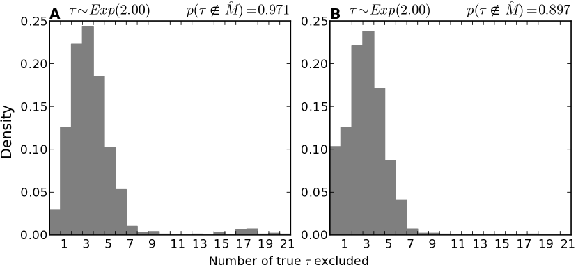
Figure 1: Histograms of the number of true divergence times excluded from the model preferred by the empirically informed model-averaging approach of Hickerson et al. (2014) when applied to simulated datasets in which divergence times of 22 pairs of populations are drawn from an exponential distribution, $\tau\sim Exp(2)$. The plots represent (A) unadjusted and (B) GLM-adjusted estimates from 1000 simulation replicates analyzed using $5\times 10^{6}$ samples from the prior. The proportion of simulation replicates in which at least one true parameter value is excluded from the preferred model ($p(\tau\notin\hat{M})$) is also given.

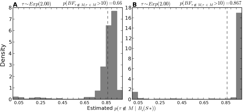
Figure 2: Histograms of the support (estimated posterior probabilities) for excluding at least one true divergence time when the empirically informed model-averaging approach of Hickerson et al. (2014) is applied to simulated datasets in which divergence times of 22 pairs of populations are drawn from an exponential distribution, $\tau\sim Exp(2)$. The plots represent (A) unadjusted and (B) GLM-adjusted estimates from 1000 simulation replicates analyzed using $5\times 10^{6}$ samples from the prior. The proportion of simulation replicates in which there is strong support for at least one true parameter value being excluded from the model ($p(BF_{\tau\notin M,\tau\in M}>10)$) is also given.

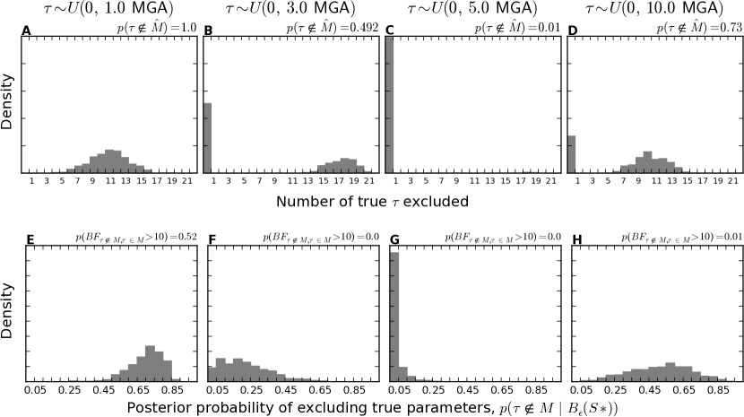
Figure 4: Histograms of the (A–D) number of true divergence times excluded from the preferred model and the (E–H) posterior probability of excluding at least one true divergence time when the empirically informed model-averaging approach of Hickerson et al. (2014) is applied to simlated datasets in which divergence times of 22 pairs of populations are randomly drawn from the uniform distributions $\tau\sim U(0,\tau_{max})$ indicated at the top of each column of plots (divergence-time distributions are given in units of millions of generations ago (MGA) assuming a per-site rate of 1$\times 10^{-8}$ mutations per generation). Four of the six $\tau_{max}$ we simulated are provided; please see Figure S6 for a summary of all of the results.

Supporting Information

Oaks, J. R., C. W. Linkem, and J. Sukumaran. Implications of uniformly distributed, empirically informed priors for phylogeographical model selection: A reply to Hickerson et al.

1 An error in Hickerson et al.’s re-analysis of the Philippines data

Hickerson et al. (2014) re-analyzed the dataset of Oaks et al. (2013) using a model-averaging approach, where they placed a discrete uniform prior over eight different prior models (see Table 1 of Hickerson et al. (2014)). However, there was an error in their methodology; their model mixes different units of time.

Each of the eight prior models used in the re-analysis by Hickerson et al. (2014) has one of two priors on the mean size of the descendant populations of each taxon pair: $\theta_{D}\sim U(0.0001,0.1)$ or $\theta_{D}\sim U(0.0005,0.04)$. As described in Oaks et al. (2013), the divergence-time parameters in the model implemented in msBayes are in generations scaled relative to a constant reference-population size, $\theta_{C}$. This reference-population size is defined in terms of the upper limit of the uniform prior on the mean size of the descendant populations, $\theta_{D}$, such that for the prior $\theta_{D}\sim U(a_{\theta_{D}},b_{\theta_{D}})$, the size of the constant reference population is $\theta_{C}=b_{\theta_{D}}/2$. Thus, the model used by Hickerson et al. (2014) mixes two different units of time. In other words, some of their prior and posterior samples are in units of $0.05/\mu$ generations, whereas others are in units of $0.02/\mu$ generations.

A fundamental assumption of the msBayes model and post hoc regression adjustment is that all possible values of the parameter of interest (divergence times) are in the same units. Thus, the results in sections “Using ABC Model Comparison to Weight Alternative Priors for the Philippine Vertebrate Data” and “Improved Sampling Efficiency by Prior Weighting Supports Asynchronous and Recent Divergence for the Philippines Vertebrate Data” and presented in Figure 2 of Hickerson et al. (2014) are invalid and should be disregarded. The error is easily illustrated by re-plotting their results with the different time units indicated (Figure S2).

2 Theoretical implications of empirical priors for Bayesian model choice—A simple example

The distinctions between Bayesian parameter estimation and model choice discussed in the main text can be illustrated with a simple example. Let us say we are interested in the fairness of a particular coin, and we denote the unknown probability of it landing heads as $\theta$. More specifically, we are interested in the probability of two models, $M_{1}$ and $M_{2}$. In both models the outcomes of flipping the coin are assumed to be binomially distributed, but under $M_{1}$ the coin is weighted toward landing heads (i.e., $\theta>0.5)$), whereas under $M_{2}$, the coin is weighted toward landing tails (i.e., $\theta<0.5$). We already have data from flipping a different coin 20 times that landed both heads and tails 10 times each, and so we decide to use these data in specifying a beta prior on fairness of the new coin of $beta(a=10,b=10)$ (Figure S1). We collect data by flipping the coin of interest $N=10$ times, $y=3$ of which land heads. Given the beta distribution is a conjugate prior for a binomial likelihood, the posterior distribution has the nice analytical form $\theta\,|\,y,N\sim beta(a+y,b+N-y)$, which for the new dataset is simply $beta(13,17)$ (Figure S1). The maximum a posteriori (MAP) estimate of the probability of heads is 0.429, and following Equation 2 in the main text the marginal likelihoods of our models of interest are

$$p(y=3,N=10\,|\,M_{1})=\int_{0.5}^{1}p(y=3,N=10\,|\,\theta,M_{1})p(\theta\,|\,M_{1})d\theta\approx 0.029,$$ (4)

and

$$p(y=3,N=10\,|\,M_{2})=\int_{0}^{0.5}p(y=3,N=10\,|\,\theta,M_{2})p(\theta\,|\,M_{2})d\theta\approx 0.097.$$ (5)

Given the models have equal probability under our prior, we can calculate the posterior probability of Model 1 as

$$p(M_{1}\,|\,y=3,N=10)=\frac{p(y=3,N=10\,|\,M_{1})}{p(y=3,N=10\,|\,M_{1})+p(y=3,N=10\,|\,M_{2})}\approx 0.23.$$ (6)

This is the correct posterior probability of Model 1 given our prior and data.

To give the data more weight relative to the prior, we could use it twice, and calculate an empirical Bayes estimate using a prior of $beta(13,17)$. This results in a “posterior” distribution of $beta(16,24)$ (Figure S1), with a MAP estimate of 0.395, and $p(M_{1}\,|\,y=3,N=10)=0.10$. The estimated posterior distribution of the parameter, and resulting MAP estimate, is similar whether or not an empirically informed prior is used. However, the posterior probability of Model 1 is very sensitive to the empirical prior, decreasing by 56%. By using the empirically informed prior, we ignored prior uncertainty, leading to an underestimate of our posterior uncertainty (Figure S1). While this did not greatly affect our estimate of $\theta$, it misled us to be overconfident in Model 2.

3 Validation analyses

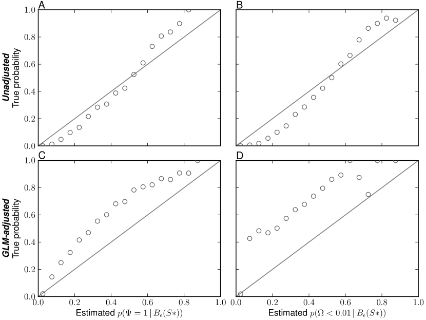
Figure 8: An assessment of the approximate Bayesian model-averageing approach of Hickerson et al. (2014) under the ideal conditions when the prior model is correct (i.e., the datasets are simulated from parameters drawn from the same prior distributions used in the analysis). The plots show the relationship between the estimated posterior and true probability of (A & C) $\Psi=1$ and (B & D) $\Omega<0.01$, based on 50,000 simulations. The results summarize the (A & B) unadjusted and (C & D) GLM-adjusted posterior estimate from each simulation replicate. The prior settings for all replicates included five prior models with $\theta_{D}\sim U(0.0001,0.1)$ and $\theta_{A}\sim U(0.0001,0.05)$ for all five models, and $M_{1}:\tau\sim U(0,0.1)$, $M_{2}:\tau\sim U(0,1)$, $M_{3}:\tau\sim U(0,5)$, $M_{4}:\tau\sim U(0,10)$, and $M_{5}:\tau\sim U(0,20)$. The number of samples from the prior was $2.5\times 10^{6}$. The simulated data structure was 8 population pairs, with a single 1000 bp locus sampled from 10 individuals from each population. The 50,000 estimates of the posterior probability of one divergence event were assigned to 20 bins of width 0.05. The estimated posterior probability of each bin is plotted against the proportion of replicates in that bin with a true value consistent with one divergence event (i.e., $\Psi=1$ or $\Omega<0.01)$.

Following Oaks et al. (2013), we characterize the model-choice behavior of the model-averaging approach of Hickerson et al. (2014) under the ideal conditions where the prior is correct (i.e., the data are generated from parameters drawn from the same prior distributions used in the analysis). We used the same prior models as above ($M_{1}$–$M_{5}$; Table 1), and simulated 50,000 datasets under this prior (10,000 from each model). We used a simulated data structure of eight population pairs, with a single 1000 base-pair locus sampled from 10 individuals from each population. We then analyzed each of these replicate datasets using the same prior with 2.5 million samples (500,000 from each of the five prior models), retaining 1000 posterior samples. Our results are very similar to Oaks et al. (2013), but we note that they are not directly comparable as our simulations contained eight population pairs rather than 10 (Figure 8). We find that the approach of Hickerson et al. (2014) estimates the posterior probability of divergence models reasonably well when all assumptions of the method are met (i.e., the prior is correct) and the unadjusted posterior estimates are used. Similar to Oaks et al. (2013), we find that the regression-adjusted estimates of the model probabilities are biased.

4 A difficult inference problem

In the main text, we discuss how the prior assumption of uniformly distributed divergence times in msBayes leads to posteriors that are difficult to interpret. However, it is also important to consider the difficult inference problem with which msBayes is faced. When applying msBayes to the dataset of Oaks et al. (2013) with 22 taxon pairs, there are 581–602 free parameters that model highly stochastic coalescent and mutational processes. Under this rich stochastic model, the method is estimating the probability of 1002 divergence models (i.e., the number of integer partitions of $Y=22$; Oaks et al., 2013). Furthermore, all the information in the sequence alignment of each taxon pair is distilled into four summary statistics. This gives us a total of 88 summary statistics (four from each of the 22 taxon pairs) that contain minimal information about many of the $\approx 600$ parameters in the model. More summary statistics can be used in msBayes, but most are highly correlated with the four default statistics, and thus contribute little additional information about the parameters from the sequence data. The large number of parameters and divergence models relative to the amount of information in the data is undoubtedly another reason the method lacks robustness to prior conditions.

5 Additional clarifications from Hickerson et al. (2014)

5.1 Saturation of summary statistics

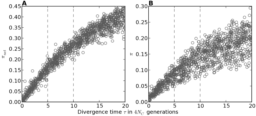
Figure 9: The summary statistics $\pi$ (Tajima, 1983) and $\pi_{net}$ (Takahata and Nei, 1985) as a function of divergence time between populations. Each plot represents 1100 pairs of parameter draws and summary statistics calculated from the simulated data. Prior settings for the simulations were $\tau\sim U(0,20)$, $\theta_{D}\sim U(0.0005,0.04)$, and $\theta_{A}\sim U(0.0005,0.02)$.

Hickerson et al. (2014) claim the priors used by Oaks et al. (2013) “cause much of the explored parameter space to be beyond the threshold of saturation in most mtDNA genes.” To explore this possibility, we simulated datasets under prior settings that match two of the three priors used by Oaks et al. (2013): $\theta_{D}\sim U(0.0005,0.04)$ and $\theta_{A}\sim U(0.0005,0.02)$. Under this prior, we randomly sample divergence-time parameters from a uniform distribution of $U(0,20)$ coalescent units, simulate datasets, and plot the $\tau$ values against the summary statistics calculated from the resulting datasets (Figure 9). Clearly, the priors used by Oaks et al. (2013) with upper limits on $\tau$ of five and 10 coalescent units suffered little to no effect from saturation. Even at divergence times of 20 coalescent units, there is still signal in the summary statistics used by msBayes (Figure 9). Thus, the assertion of Hickerson et al. (2014) that the priors used by Oaks et al. (2013) sample parameter space in which the mtDNA alignments are saturated by substitutions is incorrect and, as a result, does not explain the bias they found.

5.2 Graphical prior comparisons

Hickerson et al. (2014) advocate the use graphical checks of prior models. This prior-predictive approach entails generating a small number (1000) of random samples from the prior and plotting the resulting summary statistics in comparison to the observed statistics to see if they coincide (see Figure 1 of Hickerson et al. (2014)). Given the richness of the msBayes model ($\approx 600$ parameters for the Philippine dataset analyzed by Hickerson et al. (2014)), we do not expect that 1000 random draws from the vast prior parameter space will yield data and summary statistics consistent with the observed data. In fact, when such random draws are tightly clustered around the observed statistics, this can be an indication that the prior is over-fit, as we show in the main text (Table 1 and Figure S3). Thus, using such plots to select priors should be avoided, and the use of posterior-predictive analyses would be much more informative about the overall fit of models.

5.3 Differing utilities of $\Psi$ and $\Omega$ in msBayes

The primary component of the msBayes model is the vector of divergence times for each of the taxon pairs, $\boldsymbol{\tau}=\{\tau_{1},\ldots,\tau_{Y}\}$ (Oaks et al., 2013). Hickerson et al. (2014) argue that the dispersion index of this vector, $\Omega$, is a better model-choice estimator than the number of divergence-time parameters within the vector, $\Psi$. They present a plot of $\Psi$ against $\Omega$ (Fig. S1 of Hickerson et al. (2014)), which is essentially a plot of sample size versus variance. This plot shows that $\Omega$ has very little information about the number of divergences among taxa. Nonetheless, Hickerson et al. (2014) conclude $\Omega$ is more informative and biogeographically relevant than $\Psi$. However, the number of divergence-time parameters within the vector and their values contains all of the information about the temporal distribution of divergences, and is much more informative than the variance (i.e., the dispersion index is not a sufficient statistic for $\boldsymbol{\tau}$). Hickerson et al. (2014) also argue that msBayes can estimate $\Omega$ much better than $\Psi$. However, Oaks et al. (2013) demonstrate that even when all assumptions of the model are met, $\Omega$ is a poor model-choice estimator (see plots B, D & F of Figure 4 in Oaks et al. (2013)), whereas $\Psi$ performs better.

Importantly, $\Omega$ is limited to estimating the probability of only a single model (the one-divergence model), and thus its utility for model-choice is very limited. I.e., it can only be informative about the probability of whether there is one divergence shared among the taxa ($\Omega=0.0$) or there is greater than one divergence ($\Omega>0.0$). As a result, not only is its model-choice utility limited, but it is also very difficult to estimate. $\Omega$ can range from zero to infinity, and the point density that it is at its lower limit of zero will always be zero. Thus, an arbitrary threshold (0.01 is used throughout the msBayes literature) must be chosen to make the probability of “simultaneous” divergence estimable. Even with this arbitrary threshold, it is still not surprising to see that it is numerically difficult to obtain reliable estimates of the probability that $\Omega$ is “near” its lower limit of zero. It is easier, less subjective, and more interpretable to estimate the probability of the model with one divergence-time parameter (i.e., $\Psi=1$). Thus, it is not surprising that Oaks et al. (2013) find that $\Psi$ is a better estimator of model probability than $\Omega$.

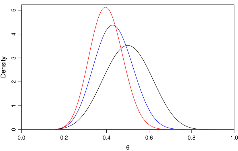
Figure 1: A plot of three beta probability density functions that represent a prior (black; $beta(10,10)$), posterior (blue; $beta(13,17)$), and empirical Bayes density (red; $beta(16,24)$) for a dataset of 10 coin flips, three of which are successes.

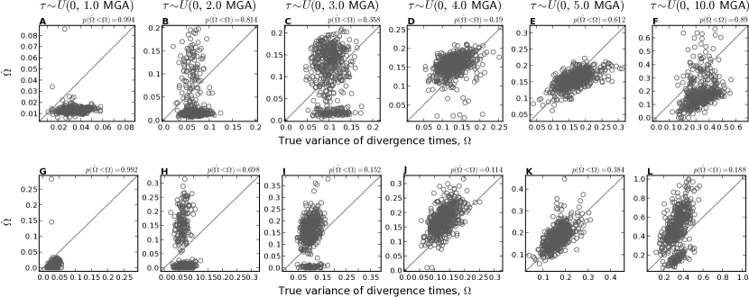
Figure 4: The accuracy of (A–F) unadjusted and (G–L) GLM-adjusted estimates of the dispersion index of divergence times ($\Omega$) when the empirically informed model-averaging approach of Hickerson et al. (2014) is applied to simlated datasets in which divergence times of 22 pairs of populations are randomly drawn from the uniform distributions $\tau\sim U(0,\tau_{max})$ indicated at the top of each column of plots (divergence-time distributions are given in units of millions of generations ago (MGA) assuming a per-site rate of 1$\times 10^{-8}$ mutations per generation).

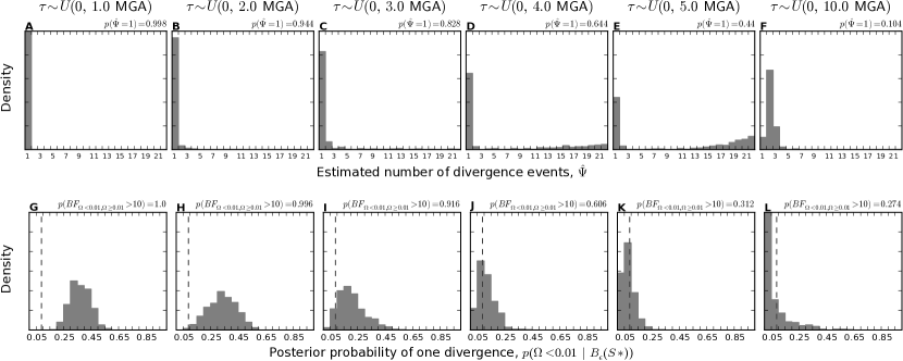
Figure 5: The tendency of the empirically informed model-averaging approach of Hickerson et al. (2014) to (A–F) infer clustered divergences and (G–L) support the extreme model of one divergence when applied to simulated datasets in which the divergence times of 22 pairs of populations are randomly drawn from the uniform distributions $\tau\sim U(0,\tau_{max})$ indicated at the top of each column of plots (divergence-time distributions are given in units of millions of generations ago (MGA) assuming a per-site rate of 1$\times 10^{-8}$ mutations per generation).

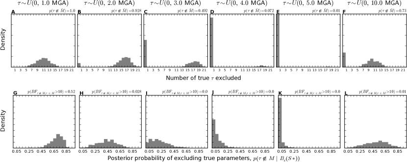
Figure 6: Histograms of the (A–F) number of true divergence times excluded from the preferred model and the (G–L) posterior probability of excluding at least one true divergence time when the empirically informed model-averaging approach of Hickerson et al. (2014) is applied to simlated datasets in which divergence times of 22 pairs of populations are randomly drawn from the uniform distributions $\tau\sim U(0,\tau_{max})$ indicated at the top of each column of plots (divergence-time distributions are given in units of millions of generations ago (MGA) assuming a per-site rate of 1$\times 10^{-8}$ mutations per generation).

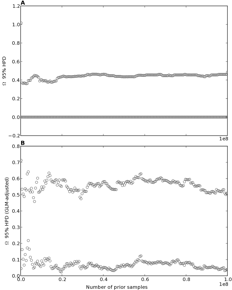
Figure 7: Traces of the estimated lower and upper limits of the 95% highest posterior density (HPD) interval of $\Omega$ (the dispersion index of divergence times) as 100 million prior samples are accumulated. Each pair of points is based on 1000 posterior samples retained from the prior. Both (A) unadjusted and (B) GLM-regression-adjusted estimates are shown. The data analyzed were the 22 pairs of Philippine taxa from Oaks et al. (2013). Prior settings were $\tau\sim U(0,10)$, $\theta_{D}\sim U(0.0005,0.04)$, and $\theta_{A}\sim U(0.0005,0.02)$.

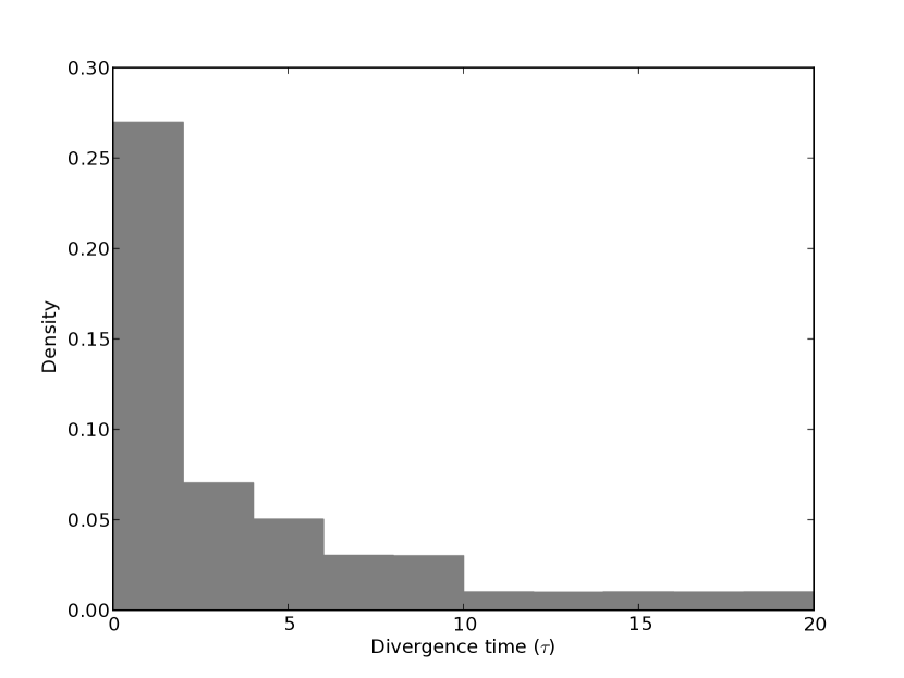
Figure 10: The prior distribution on divergence times imposed by the model-averaging prior comprised of five models with different uniform priors on $\tau$: $M_{1}$ ($\tau\sim U(0,0.1)$), $M_{2}$ ($\tau\sim U(0,1)$), $M_{3}$ ($\tau\sim U(0,5)$), $M_{4}$ ($\tau\sim U(0,10)$), $M_{5}$ ($\tau\sim U(0,20)$).

References

- Barber and Klicka (2010) Barber, B. R. and J. Klicka, 2010. Two pulses of diversification across the Isthmus of Tehuantepec in a montane Mexican bird fauna. Proceedings Of The Royal Society B-Biological Sciences 277:2675–2681.
- Bell et al. (2012) Bell, R. C., J. B. MacKenzie, M. J. Hickerson, K. L. Chavarria, M. Cunningham, S. Williams, and C. Moritz, 2012. Comparative multi-locus phylogeography confirms multiple vicariance events in co-distributed rainforest frogs. Proceedings Of The Royal Society B-Biological Sciences 279:991–999.
- Carlin and Gelfand (1990) Carlin, B. P. and A. E. Gelfand, 1990. Approaches for empirical Bayes confidence intervals. Journal of the American Statistical Association 85:105–114.
- Carnaval et al. (2009) Carnaval, A. C., M. J. Hickerson, C. F. B. Haddad, M. T. Rodrigues, and C. Moritz, 2009. Stability Predicts Genetic Diversity in the Brazilian Atlantic Forest Hotspot. Science 323:785–789.
- Chan et al. (2011) Chan, L. M., J. L. Brown, and A. D. Yoder, 2011. Integrating statistical genetic and geospatial methods brings new power to phylogeography. Molecular Phylogenetics and Evolution 59:523–537.
- Chan et al. (2014) Chan, Y. L., D. Schanzenbach, and M. J. Hickerson, 2014. Detecting concerted demographic response across community assemblages using hierarchical approximate Bayesian computation. Molecular Biology and Evolution 31:2501–2515.
- Daza et al. (2010) Daza, J. M., T. A. Castoe, and C. L. Parkinson, 2010. Using regional comparative phylogeographic data from snake lineages to infer historical processes in Middle America. Ecography 33:343–354.
- Efron (2008) Efron, B., 2008. Microarrays, Empirical Bayes and the Two-Groups Model. Statistical Science 23:1–22.
- Efron (2013) ———, 2013. Empirical bayes modeling, computation, and accuracy. Manuscript AMS 2010 subject classifications: Primary 62C10; secondary 62-07, 62P10.
- Hickerson et al. (2006) Hickerson, M. J., E. A. Stahl, and H. A. Lessios, 2006. Test for simultaneous divergence using approximate Bayesian computation. Evolution 60:2435–2453.
- Hickerson et al. (2014) Hickerson, M. J., G. N. Stone, K. Lohse, T. C. Demos, X. Xie, C. Landerer, and N. Takebayashi, 2014. Recommendations for using msbayes to incorporate uncertainty in selecting an ABC model prior: A response to Oaks et al. Evolution 68:284–294.
- Huang et al. (2011) Huang, W., N. Takebayashi, Y. Qi, and M. J. Hickerson, 2011. MTML-msBayes: Approximate Bayesian comparative phylogeographic inference from multiple taxa and multiple loci with rate heterogeneity. BMC Bioinformatics 12:1.
- Hwang et al. (2009) Hwang, J. T. G., J. Qiu, and Z. Zhao, 2009. Empirical Bayes confidence intervals shrinking both means and variances. Journal of the Royal Statistical Society Series B-Statistical Methodology 71:265–285.
- Jeffreys (1939) Jeffreys, H., 1939. Theory of Probability. 1st ed. Clarendon Press, Oxford, U.K.
- Laird and Louis (1987) Laird, N. M. and T. A. Louis, 1987. Empirical Bayes confidence intervals based on bootstrap samples. Journal of the American Statistical Association 82:739–750.
- Laird and Louis (1989) ———, 1989. Empirical Bayes confidence intervals for a series of related experiments. Biometrics 45:481–495.
- Lawson (2010) Lawson, L. P., 2010. The discordance of diversification: evolution in the tropical-montane frogs of the Eastern Arc Mountains of Tanzania. Molecular Ecology 19:4046–4060.
- Leaché et al. (2007) Leaché, A. D., S. C. Crews, and M. J. Hickerson, 2007. Two waves of diversification in mammals and reptiles of Baja California revealed by hierarchical Bayesian analysis. Biology Letters 3:646–650.
- Lindley (1957) Lindley, D. V., 1957. A statistical paradox. Biometrika 44:187–192.
- Morris (1983) Morris, C. N., 1983. Parametric empirical bayes inference: Theory and applications. Journal of the American Statistical Association 78:47–55.
- Oaks (2014) Oaks, J. R., 2014. An improved approximate-bayesian model-choice method for estimating shared evolutionary history. BMC Evolutionary Biology 14:150.
- Oaks et al. (2013) Oaks, J. R., J. Sukumaran, J. A. Esselstyn, C. W. Linkem, C. D. Siler, M. T. Holder, and R. M. Brown, 2013. Evidence for climate-driven diversification? a caution for interpreting ABC inferences of simultaneous historical events. Evolution 67:991–1010.
- Plouviez et al. (2009) Plouviez, S., T. M. Shank, B. Faure, C. Daguin-Thiebaut, F. Viard, F. H. Lallier, and D. Jollivet, 2009. Comparative phylogeography among hydrothermal vent species along the East Pacific Rise reveals vicariant processes and population expansion in the South. Molecular Ecology 18:3903–3917.
- Stone et al. (2012) Stone, G. N., K. Lohse, J. A. Nicholls, P. Fuentes-Utrilla, F. Sinclair, K. Schönrogge, G. Csóka, G. Melika, J.-L. Nieves-Aldrey, J. Pujade-Villar, M. Tavakoli, R. R. Askew, and M. J. Hickerson, 2012. Reconstructing community assembly in time and space reveals enemy escape in a Western Palearctic insect community. Current Biology 22:532–537.
- Tajima (1983) Tajima, F., 1983. Evolutionary relationship of DNA sequences in finite populations. Genetics 105:437–460.
- Takahata and Nei (1985) Takahata, N. and M. Nei, 1985. Gene genealogy and variance of interpopulational nucleotide differences. Genetics 110:325–344.
- Voje et al. (2009) Voje, K. L., C. Hemp, Ø. Flagstad, G.-P. Saetre, and N. C. Stenseth, 2009. Climatic change as an engine for speciation in flightless Orthoptera species inhabiting African mountains. Molecular Ecology 18:93–108.
fig0cm2.2cm \cftpagenumbersofffig