Nonequilibrium steady state of the kinetic Glauber-Ising model under an alternating magnetic field

Abstract

When periodically driven by an external magnetic field, a spin system can enter a phase of steady entrained oscillations with nonequilibrium probability distribution function. We consider an arbitrary magnetic field switching its direction with frequency comparable with the spin-flip rate and show that the resulting nonequilibrium probability distribution can be related to the system equilibrium distribution in the presence of a constant magnetic field of the same magnitude. We derive convenient approximate expressions for this exact relation and discuss their implications.

I Introduction

The equilibrium properties of a statistical-physical system are often characterized by a few macroscopic degrees of freedom. As the system gets out of equilibrium, however, a huge, mostly unmanageable number of degrees of freedom come into play. For this reason, most conventional approaches to nonequilibrium physics have recourse to the linear-response approximation, where the response of the system to a small perturbation is expressed in terms of equilibrium properties. The possibility of an exact formalism incorporating nonequilibrium processes has recently emerged with the discovery of the so-called fluctuation theorems Evans et al. (1993); *cohen; *jar; *crooks and the formulation of steady-state thermodynamics Oono and Paniconi (1998); *hatano; *koma; *koma2. Popular study cases of collective nonequilibrium dynamics are provided by classical spin models, such as the kinetic Glauber-Ising model Glauber (1963). In addition to the earlier literature, where the dynamical phase transitions in such low dimensional stylized systems have been investigated at depth Sides et al. (1998a); *sides1; *sides3; Korniss et al. (2000); *korniss1; Robb et al. (2007); Park and Pleimling (2012); *park2, we focus here on a different aspect of the problem, namely on the search for an algebraic framework to characterize a nonequilibrium steady state (NESS). This class of systems can be maintained out of equilibrium by a variety of external agents, like multiple heat reservoirs Lavrentovich and Zia (2010) or external time-dependent magnetic fields Tomé and de Oliveira (1990). For instance, when a weak, slowly oscillating magnetic field is applied to the Glauber-Ising model, the system eventually enters a steady collective oscillation phase via entrainment. The linear-response theory accurately describes the onset of entrainment by adopting the average magnetization as an order parameter Leung and Néda (1998); *double; *double2. However, we show below that such a perturbation approach fails to determine the probability density function (PDF) itself or other observables that are nonlinear functions of the PDF, like the entropy.

The approach pursued in this work is opposite to the linear-response theory: Instead of restricting ourselves to the low-frequency regime, where the magnetic field oscillates with a period much longer than the spin-flip time scale, here we assume from the beginning a high-frequency regime, where the driving frequency and the spin-flip rate are comparable. We show that, even if this situation occurs far from equilibrium, there exists a rather simple relationship between the NESS for the driven spin system, and the known Boltzmann equilibrium PDF for the system subject to a constant magnetic field. This result can be then extended to analyze more realistic situations for lower driving frequency. In this first report, we focus on globally coupled spin systems, whose critical behavior belongs to the mean-field (MF) universality class. In view of practical applications, we remind that this is the universality class of three-dimensional quantum Ising ferromagnets and uniaxial dipolar Ising ferromagnets Als-Nielsen et al. (1974); *nielsen.

This work is organized as follows: In Sec. II, we attempt a perturbative approach to obtain the NESS under sinusoidal modulation, and compare it with numerical results. In Sec. III, we present an alternative algebraic formulation for square-wave modulation at high frequency, yielding the NESS as an eigenvector. We derive an approximate expression at lower frequencies as well. After comparing our formula with numerical results, we summarize this work in Sec. IV.

II Perturbative approach

Let us consider $n$ Ising spins governed by the Glauber dynamics. The number of possible configurations is $N\equiv 2^{n}$. For each spin configuration $i=(\sigma_{1},\ldots,\sigma_{n})$, the energy function is

$$E_{i}=-J\sum_{\left<\mu\nu\right>}\sigma_{\mu}\sigma_{\nu}-h\sum_{\mu}\sigma_{\mu},$$ (1)

where the first summation runs over the nearest neighbors and $h$ is an external magnetic field. In the globally coupled case discussed here, every spin is coupled to all the other spins so that the first summation should be understood as running over all the spin pairs. At the same time, the coupling strength $J$ is replaced by $J_{0}(n-1)^{-1}$, with $J_{0}$ a constant, to ensure that the energy is an extensive quantity. According to the Glauber dynamics, the transition rate from the spin configurations $i=(\sigma_{1},\ldots,\sigma_{\alpha},\ldots\sigma_{n})$ to $j=(\sigma_{1},\ldots,-\sigma_{\alpha},\ldots\sigma_{n})$ is

$$w_{ji}=\frac{1}{2n}\left[1-\sigma_{\alpha}\tanh\left(\beta J\sum_{k\neq\alpha}\sigma_{k}+\beta h\right)\right],$$ (2)

with $\beta\equiv(k_{B}T)^{-1}$ and $T$ denoting the temperature of the heat bath in contact with this system. To simplify notation, in the following we set $J_{0}=1$ and $k_{B}=1$. The prefactor $n^{-1}$ in Eq. (2) indicates that only one spin was flipped. In terms of these transition rates, one can write the master equation

$$\Delta p_{i}(t)=\Delta t\sum_{j\neq i}^{N}[w_{ij}(h)p_{j}(t)-w_{ji}(h)p_{i}(t)],$$ (3)

where $p_{i}$ is the probability to observe the configuration $i$ and $\Delta t$ is the average spin-flip time. The system PDF, denoted by the vector $\mathbf{p}$, with transpose $\mathbf{p}^{T}=(p_{1},\ldots,p_{N})$, is normalized to $1$, i.e., $\sum_{j=1}^{N}p_{j}=1$. This is one of the simplest systems exhibiting nontrivial collective behavior such as dynamic phase transitions and hysteresis Chakrabarti and Acharyya (1999). If the external field is absent, the phase transition occurs at $T=1$ in units of $J_{0}/k_{B}$ in the thermodynamic limit.

We show first that standard linear perturbation analysis fails to reproduce the $h$ dependence of $\mathbf{p}$, even for very small system sizes. For a system of two spins, $n=2$, there exist $N=4$ possible states, namely, $++,+-,-+$, and $--$. Equivalently, we label these states $3,2,1$, and $0$, by digitizing the spin directions $+$ and $-$, respectively, as $1$ and $0$. At low fields, $\beta h\ll 1$, the transition rates $w_{ji}$ can be expanded in powers of $\beta h$, so that $p_{i}(t)$ deviates from its equilibrium value, $p_{i}^{\ast}$ at $h=0$, by a small amount $\eta_{i}$,

$$p_{i}(t)=p_{i}^{\ast}+\eta_{i}(t),$$ (4)

with $p_{3}^{\ast}=p_{0}^{\ast}=[2(1+e^{-2\beta})]^{-1}$, $p_{1}^{\ast}=p_{2}^{\ast}=[2(1+e^{2\beta})]^{-1}$, and $\sum_{i}\eta_{i}(t)=0$. By retaining all terms up to the first order in $\eta_{i}$ and $\beta h$, the time evolution of $\mathbf{\eta}$, with $\mathbf{\eta}^{T}\equiv(\eta_{3},\eta_{2},\eta_{1},\eta_{0})$, is governed by the linear equation $d\mathbf{\eta}/dt=\tilde{W}^{\ast}\cdot\mathbf{\eta}+\left(\frac{1}{4}\beta h~{}{\rm sech}^{2}\beta\right)\mathbf{\phi}$, obtained by taking the limit $\Delta t\rightarrow 0$ in Eq. (3). Here, we have introduced the transition matrix at $h=0$, $\tilde{W}^{\ast}$, and a coupling vector $\mathbf{\phi}$, with $\mathbf{\phi}^{T}=(1,0,0,-1)$. The matrix $\tilde{W}^{\ast}$ has eigenvalues $\zeta_{3}=-1$, $\zeta_{2}=0$, $\zeta_{1}=\frac{1}{2}(-1-\tanh\beta)$, and $\zeta_{0}=\frac{1}{2}(-1+\tanh\beta)$, and the corresponding eigenvectors are the columns of the diagonalization matrix $\tilde{Y}$. After diagonalizing $W^{\ast}$ with $\tilde{Y}$, the equation for $\eta_{i}(t)$ reads

$$\frac{d}{dt}\eta^{\prime}_{i}=\zeta_{i}\eta^{\prime}_{i}-\delta_{i0}\frac{\beta h}{4}{\rm sech}^{2}\beta,$$ (5)

where the prime sign labels the transformed coordinates and $\delta_{i0}$ is the Kronecker $\delta$ function. As $h(t)$ is assumed next to vary slowly in time, in leading order, terms proportional to $dh/dt$ can be safely discarded. In the case of sinusoidally oscillating fields, $h(t)=h_{0}\sin\omega t$, we can easily solve the set of linear differential equations in Eq. (5) for large $t$ and transform the solutions back to the original coordinates, namely, $\eta_{1}=\eta_{2}=0$ and $\eta_{0}=\frac{1}{4}\beta h_{0}{\rm sech}^{2}\beta(\omega\cos\omega t+\zeta_{0}\sin\omega t)/(\zeta_{0}^{2}+\omega^{2})=-\eta_{3}$. Note that $h(t)$ is only coupled to the eigenmode associated with the second largest eigenvalue $\zeta_{0}$ [see Fig. 1(a)]. At larger $n$, the relaxation time toward $p_{i}^{\ast}$ is still determined by the second largest eigenvalue $\zeta_{0}$ (i.e., the slowest decaying mode) [Fig. 1(b)]. As $n$ grows, the critical point will roughly correspond to the resonance condition $|\zeta_{0}|\approx\omega\rightarrow 0$, where the time scale diverges, so that the ground state associated with $\zeta_{2}=0$ becomes doubly degenerate.

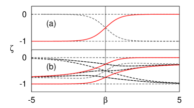
Figure 1: (Color online) Eigenvalue spectrum of the transition matrix at $h=0$, $\tilde{W}^{\ast}$, for (a) $n=2$ and (b) $n=4$. The solid lines represent the eigenvalues coupled to $h$, according to the linear-response theory (see text). The negative-$\beta$ side represents the antiferromagnetic Ising model Vives et al. (1997).

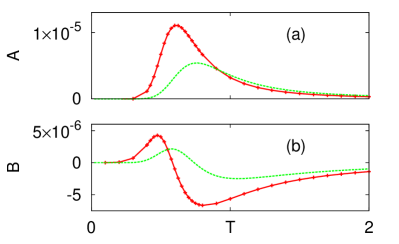
Figure 2: (Color online) Amplitudes of entropy change for $n=2$, $\omega=2\pi\times 10^{-2}$, and $h_{0}=10^{-2}$. The line points show $A$ and $B$ of $d\langle S\rangle/dt$ [see Eq. (6)] obtained by numerically integrating Eq. (3) with $\Delta t=10^{-2}$, while the dotted lines represent the corresponding analytic results in the linear-response theory.

We quantify now the system response to the external drive $h(t)$ by calculating its entropy change as a function of time Tomé (2006); *tome10; *tome. In this case, the nonequilibrium entropy can be expressed as $\left<S\right>=-\sum_{i}p_{i}\ln p_{i}$ and approximated to $-\sum_{i}p_{i}^{\ast}\ln p_{i}^{\ast}-\eta_{3}^{2}/p_{3}^{\ast}$. By inserting our estimate for $\eta_{3}$, we obtain the rate of entropy change per spin,

$$\frac{1}{n}\frac{d\left<S\right>}{dt}\approx A\cos 2\omega t+B\sin 2\omega t,$$ (6)

where in the linear-response theory $A^{\rm lin}\equiv-2\beta^{2}e^{2\beta}\zeta_{0}h_{0}^{2}\omega^{2}/C$ and $B^{\rm lin}\equiv\beta^{2}e^{2\beta}h_{0}^{2}\omega(-\zeta_{0}^{2}+\omega^{2})/C$ with $C\equiv(1+e^{2\beta})^{3}(\zeta_{0}^{2}+\omega^{2})^{2}$. Since the system entropy is a periodic function of time, differently from the entropy production of the total process Tomé (2006); *tome10; *tome, the rate in Eq. (6) has no definite sign. Note that, for a given $\beta$, $A^{\rm lin}$ attains a maximum at $\omega=|\zeta_{0}|$, as anticipated above. However, when compared with the numerical data displayed in Fig. 2, Eq. (6) clearly fails for $\beta h\gtrsim O(10^{-2})$. The discrepancy gets even worse as the system size increases. The failure of the linear-response theory is consistent with the observation that at low $T$, in the large-$n$ limit, the system PDF may experience singular changes for infinitesimal field modulations Goldenfeld (1993), which invalidates the assumption of Eq. (4) for $\beta h\ll 1$.

III Algebraic formulation

III.1 High-frequency modulation

We introduce now an alternative approach aimed at overcoming the limitations of the linear-response theory. The main idea is that the up-down symmetry will be generally broken in the presence of the external field, even though the field is oscillating, so that it is better to choose a symmetry-broken equilibrium state as our starting point to study the NESS *[See][; forasimilarapproachtotheKondoeffectinaNESS.]jhong. This can be best explained in terms of linear algebra in the following way: Let $U(h)$ denote the transition matrix for a spin system of energy function as in Eq. (1), subject to an external magnetic field $h$. Under a static field $+h$, the corresponding system dynamics is formulated as an $N\times N$ matrix equation, $\mathbf{p}(t+\Delta t)=U(+h)\cdot\mathbf{p}(t)$, with a steady-state solution coinciding with the eigenvector associated with the largest eigenvalue, $\lambda_{1}=1$, that is $\mathbf{q_{1}}=U(+h)\cdot\mathbf{q_{1}}$. After normalization, this determines the system equilibrium PDF at constant $h$. The existence and uniqueness of the eigenvector $\mathbf{q}_{1}$ for any finite $n$ is ensured by the Perron-Frobenius theorem Meyer (2000). We hereafter assume finite $n$ and full knowledge of the $U(+h)$ spectrum, i.e., of all eigenmodes $\mathbf{q}_{i}$ as solutions of the matrix equation $U(+h)\cdot\mathbf{q}_{i}=\lambda_{i}\mathbf{q}_{i}$, with $\mathbf{q}_{i}^{T}\cdot\mathbf{q}_{i}=1$ and $\lambda_{i}$ denoting the $i$th largest eigenvalue. If the field changes its sign at every time step, $\Delta t$, with constant magnitude, then the time evolution of the PDF obeys the equation

$$\mathbf{p}(t+2\Delta t)=U(-h)\cdot U(+h)\cdot\mathbf{p}(t).$$ (7)

Equation (7) describes the fastest oscillating field that a discrete-time formulation with time step $\Delta t$ can accommodate (see, e.g., Ref. Verley et al. (2013)). To make notation more compact, we define $U^{\pm}\equiv U(\pm h)$. These two matrices are related by a similarity transformation $U^{-}=P\cdot U^{+}\cdot P$, where $P$ is a permutation matrix exchanging the $h$ direction from $+$ to $-$ and vice versa. Note that $P^{2}=I$, $I$ being the identity matrix. Accordingly, Eq. (7) can be rewritten as $\mathbf{p}(t+2\Delta t)=P\cdot U^{+}\cdot P\cdot U^{+}\cdot\mathbf{p}(t)=[P\cdot U^{+}]^{2}\cdot\mathbf{p}(t)$. Under steady-state conditions, the system PDF is given by the solution $\tilde{\mathbf{p}}$ of the following equation:

$$\tilde{\mathbf{p}}=P\cdot U^{+}\cdot\tilde{\mathbf{p}},$$ (8)

with the system alternating between $\tilde{\mathbf{p}}$ and $P\cdot\tilde{\mathbf{p}}$ at every time step. When replacing $[P\cdot U^{+}]^{2}$ by $[P\cdot U^{+}]$ in the right-hand side (rhs) of Eq. (8), one might argue that $\mathbf{p}(t+\Delta t)=\pm P\cdot U^{+}\cdot\mathbf{p}(t)$; However as all elements in $P$, $U^{+}$, and $\tilde{\mathbf{p}}$ are non-negative, the $+$ sign is the correct choice. Since $P$ is a known matrix and $U^{+}$ was assumed to be known, one expects that the NESS, $\tilde{\mathbf{p}}$, and the equilibrium PDF associated with $U^{+}$, $\mathbf{q_{1}}$, are algebraically related. The desired relationship can be established by multiplying Eq. (8) times $P$ and subtracting $\tilde{\mathbf{p}}$ from both sides to get $(U^{+}-I)\cdot\tilde{\mathbf{p}}=(P-I)\cdot\tilde{\mathbf{p}}$. Unfortunately, $(U^{+}-I)$ is non-invertible because the largest eigenvalue $\lambda_{1}=1$ requires $\det(U^{+}-\lambda_{1}I)=0$. One circumvents this difficulty by analyzing the subspace orthogonal to $\mathbf{q}_{1}$, i.e., rewriting $\tilde{\mathbf{p}}$ as

$$\tilde{\mathbf{p}}=X_{\epsilon}\cdot\tilde{\mathbf{p}}+c~{}\mathbf{q}_{1},$$ (9)

where the sparse matrix $\epsilon$ in the projection operator $X_{\epsilon}\equiv(U^{+}-I+\epsilon)^{-1}\cdot(P-I)$ is required to make the inversion possible (see Drazin inverse in Ref. Meyer (2000)). The reason for the unknown $c$ in Eq. (9) is that this subspace retains no information about the direction of $\mathbf{q}_{1}$. A convenient choice for $\epsilon$ is as follows. Let us define a block matrix $Q\equiv(\mathbf{q}_{1},\mathbf{q}_{2},\cdots,\mathbf{q}_{N})$ so that in the transformed coordinates, $Q^{-1}\cdot(U^{+}-I)\cdot Q$ is a diagonal matrix with the first diagonal element $\lambda_{1}-1=0$. The other diagonal elements are nonzero as long as $\lambda_{k}<\lambda_{1}=1$ for $k>1$. To make the first diagonal element nonzero, we then consider a matrix with a single nonzero element $\epsilon^{\prime}_{ij}=-\delta_{i1}\delta_{j1}$, which corresponds to $\epsilon=Q\cdot\epsilon^{\prime}\cdot Q^{-1}$ in the original coordinates. Now, $Q^{-1}\cdot(U^{+}-I+\epsilon)\cdot Q$ is clearly invertible, whereas $Q^{-1}\cdot(U^{+}-I)\cdot Q$ was not, so we have explicitly constructed $X_{\epsilon}$. It is important that $\lambda_{1}$ is no eigenvalue of $X_{\epsilon}$, so that the solution of Eq. (9),

$$\tilde{\mathbf{p}}=c~{}(I-X_{\epsilon})^{-1}\cdot\mathbf{q}_{1},$$ (10)

relating $\tilde{\mathbf{p}}$ to $\mathbf{q}_{1}$ is well defined. Finally, the constant $c$ is determined by normalizing $\tilde{\mathbf{p}}$; most remarkably one can show that $\mathbf{p}^{\rm eq}\equiv c~{}\mathbf{q}_{1}$ is also a normalized PDF. This shows how $\tilde{\mathbf{p}}$ in nonequilibrium is related to the equilibrium PDF.

Note that the vector $\tilde{\mathbf{p}}$ can be expressed as a polynomial by multiplying it times the lowest common denominator of all the $N$ elements and imposing the normalization condition only at the final step; hence, $\tilde{\mathbf{p}}=\tilde{\mathbf{p}}^{(1)}+\tilde{\mathbf{p}}^{(2)}+\ldots+\tilde{\mathbf{p}}^{(n)}$, with $\tilde{\mathbf{p}}^{(k)}\propto(\Delta t)^{k}$. The idea is to construct the NESS as a series solution with a small expansion parameter $\Delta t$. Such summands are related to one another,

$$0 = (P-I)\cdot\tilde{\mathbf{p}}^{(1)},$$ (11)

$$(U^{+}-I)\cdot\tilde{\mathbf{p}}^{(1)} = (P-I)\cdot\tilde{\mathbf{p}}^{(2)},$$

$$\vdots$$

$$(U^{+}-I)\cdot\tilde{\mathbf{p}}^{(n-1)} = (P-I)\cdot\tilde{\mathbf{p}}^{(n)},$$

$$(U^{+}-I)\cdot\tilde{\mathbf{p}}^{(n)} = 0.$$ (12)

This set of equations can also be written as

$$(U^{+}-I)\cdot\tilde{\mathbf{p}}^{(k-1)}=(P-I)\cdot\tilde{\mathbf{p}}^{(k)},$$ (13)

with $\tilde{\mathbf{p}}^{(k)}\equiv 0$ if $k\leq 0$ or $k>n$. It is clearly seen that one obtains the original equation to solve [Eq. (8)] when summing up both sides. Since Eq. (12) should have a solution proportional to $\mathbf{q}_{1}$, which is known to us by assumption, one may attempt to proceed recursively from Eq. (12) all the way up to Eq. (11). Still, the singular matrix $(U^{+}-I)$ does not allow the direct inversion but leaves an undetermined component proportional to $\mathbf{q}_{1}$ every time. Adding up these recursive solutions with the undetermined parts, we end up with our key result, Eq. (9). To avoid lengthy algebraic manipulations, we limit ourselves to a hand-waving argument for the recursive Eq. (13). As the matrix $U^{+}$ is of the form $U^{+}=I+\Delta t~{}W$, with $W\equiv\{w_{ij}\}$, multiplying $\tilde{\mathbf{p}}^{(k-1)}\propto(\Delta t)^{k-1}$ by $(U^{+}-I)$ raises the exponent of $\Delta t$ by $1$, thus relating $\tilde{\mathbf{p}}^{(k-1)}\propto(\Delta t)^{k-1}$ to $\tilde{\mathbf{p}}^{k}\propto(\Delta t)^{k}$. In addition, the matrix $(P-I)$ on the rhs guarantees that one recovers Eq. (8) when resumming both sides of Eq. (13). The truncation of the recursive Eqs. (13) at $k=n+1$ is a consequence of the MF character of the model. Indeed, for models with lower symmetry the number of recursive equations would be larger than $n+1$. In particular, the last equation implies that $\tilde{\mathbf{p}}^{(n)}$ is proportional to $\mathbf{p}^{\rm eq}$. In fact, only $\tilde{\mathbf{p}}^{(k)}$ with $k\geq n$ can be made proportional to $\mathbf{p}^{\rm eq}$ in a MF model with $n+1$ different energy levels: For Glauber’s transition rates with $w_{ij}\propto\exp[\beta(E_{j}-E_{i})]$, it takes products involving $n$ such factors to obtain a PDF proportional to $\exp(-\beta E_{i})$.

III.2 Lower-frequency modulation

We extend now our analysis to lower driving frequencies by considering the case when $h$ switches its sign every $\gamma$ time steps, so that the NESS equation to solve is now $\left(U^{+}\right)^{\gamma}\cdot\tilde{\mathbf{p}}=P\cdot\tilde{\mathbf{p}}$. In the steady state, the system goes through the transition sequences

$$\tilde{\mathbf{p}}\rightarrow U^{+}\cdot\tilde{\mathbf{p}}\rightarrow\ldots\rightarrow(U^{+})^{\gamma-1}\cdot\tilde{\mathbf{p}}\rightarrow P\cdot\tilde{\mathbf{p}}\rightarrow$$

$$U^{-}\cdot P\cdot\tilde{\mathbf{p}}\rightarrow\ldots\rightarrow(U^{-})^{\gamma-1}\cdot P\cdot\tilde{\mathbf{p}}\rightarrow\tilde{\mathbf{p}}\rightarrow\ldots.$$ (14)

As above, the steady-state solution is derived as $\tilde{\mathbf{p}}=\left[I-X_{\epsilon}(\gamma)\right]^{-1}\cdot\mathbf{p}^{\rm eq}$, with $X_{\epsilon}(\gamma)\equiv\left[(U^{+})^{\gamma}-I+\epsilon\right]^{-1}\cdot(P-I)$. Due to our choice for $\epsilon$ and using the Neumann series $(A+B)^{-1}\approx A^{-1}-A^{-1}\cdot B\cdot A^{-1}$ Meyer (2000), we can approximate $X_{\epsilon}(\gamma)$ to $X_{\epsilon}(\gamma)\approx\left[I+(U^{+})^{\gamma}+\epsilon\right]\cdot(I-P)$ and obtain

$$I-X_{\epsilon}(\gamma)\approx P+\left[(U^{+})^{\gamma}+\epsilon\right]\cdot(P-I),$$ (15)

as long as $\beta h\ll 1$ or $\gamma\gg 1$. In particular, on increasing $\gamma$, the second term on the rhs of Eq. (15) can be made much smaller than the first one. When applied to $\mathbf{p}^{\rm eq}$, the inverse of the lhs of Eq. (15) is then approximated, again through the Neumann series, to

$$\tilde{\mathbf{p}}\approx P\cdot\mathbf{p}^{\rm eq}+P\cdot\left[(U^{+})^{\gamma}+\epsilon\right]\cdot(P-I)\cdot\mathbf{p}^{\rm eq}.$$ (16)

Therefore, the leading order of $[I-X_{\epsilon}(\gamma)]^{-1}$ is $P$, and not $I$, even in the limit $h\rightarrow 0$, because $X_{\epsilon}(\gamma)$ is not small compared to $I$ Meyer (2000). The PDF $\tilde{\mathbf{p}}$ should indeed be close to $P\cdot\mathbf{p}^{\rm eq}$ because $U^{-}$ has evolved the system for $\gamma$ time steps, so that it is the second term on the rhs of Eq. (16) that describes the PDF change right after field reversal. Since $\left[(U^{+})^{\gamma}+\epsilon\right]\cdot\mathbf{p}^{\rm eq}=0$, the dominant change is proportional to $P\cdot\mathbf{q}_{2}$, whose elements add up to zero. This is consistent with the predictions (Fig. 1) of the linear-response theory, which is unable to distinguish between $\mathbf{q}_{2}$ and $P\cdot\mathbf{q}_{2}$. We note that for $\beta\ll 1$ the matrix $U^{+}$ is almost symmetric, which implies $\mathbf{q}_{2}^{T}\cdot\mathbf{p}^{\rm eq}\ll 1$. Under these conditions a simple two-eigenmode approximation allows us to go beyond the linear-response approximation, by writing

$$\tilde{\mathbf{p}}\approx\mathbf{p}^{\rm approx}\equiv P\cdot\mathbf{p}^{\rm eq}+\lambda_{2}^{\gamma}~{}[\mathbf{q}_{2}^{T}\cdot(P-I)\cdot\mathbf{p}^{\rm eq}](P\cdot\mathbf{q}_{2}).$$ (17)

We checked the validity of this scheme by computing the Kullback-Leibler divergence $D_{\rm KL}(\tilde{\mathbf{p}}||\mathbf{p}^{\rm approx})\equiv\sum_{i=1}^{N}\tilde{p}_{i}\ln\left(\tilde{p}_{i}/p^{\rm approx}_{i}\right)$. As displayed in Fig. 3, with increasing $\gamma$, $D_{\rm KL}$ decreases over the whole parameter region. This confirms that in most cases the perturbative description of Eq. (17) based on the first two eigenmodes provides a reasonable approximation for $\tilde{\mathbf{p}}$.

Figure 3: (Color online) Kullback-Leibler divergence of $\mathbf{p}^{\rm approx}$ from the exact PDF, $\tilde{\mathbf{p}}$ for $n=6$ spins; (a) $\gamma=10^{1}$ and (b) $\gamma=10^{2}$ with $\Delta t\equiv 1$. The black region in panel (a) denotes the parameter domain where Eq. (17) breaks down (i.e., yields negative probabilities).

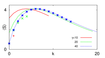
Figure 4: (Color online) Nonequilibrium entropy as a function of the number, $k$, of time steps with $\Delta t\equiv 1$, for $n=6$ and $h=1$ at temperature $T=1$. The solid curves represent the exact results for different $\gamma$; the crosses are approximate results obtained by combining Eqs. (18) and (19) (see text), and the colors indicate the corresponding values of $\gamma$. Missing crosses at large $k$ indicate a breakdown of the approximation (negative predicted probability).

Furthermore, when applied to $\mathbf{p}^{\rm eq}$, the commutator $[U^{+},P]$ can be estimated in terms of the first two PDF’s, $\tilde{\mathbf{p}}$ and $U^{+}\tilde{\mathbf{p}}$, in the transition sequence of Eq. (14), i.e.,

$$[U^{+},P]\cdot\mathbf{p}^{\rm eq}\approx(U^{+}-I)\cdot\tilde{\mathbf{p}}.$$ (18)

The time evolution of $\mathbf{p}^{\rm eq}$ is then formally expressed as

$$(U^{+})^{k}\cdot P\cdot\mathbf{p}^{\rm eq}=\left\{P+\left[\sum_{j=0}^{k-1}(U^{+})^{j}\right]\cdot[U^{+},P]\right\}\cdot\mathbf{p}^{\rm eq},$$ (19)

where we recall that for $\gamma\gg 1$ the lhs may be approximated to $(U^{+})^{k}\cdot\tilde{\mathbf{p}}$. By using Eqs. (18) and (19), we numerically computed the time dependence of $\left<S\right>$ as plotted in Fig. 4, where this approximation closely reproduces the numerical data at large $\gamma$.

The $\Delta t$ power counting rule in Eq. (13) can also be generalized by considering $\tilde{\mathbf{p}}=\tilde{\mathbf{p}}^{(1)}+\tilde{\mathbf{p}}^{(2)}+\ldots+\tilde{\mathbf{p}}^{(n\gamma)}$. The matching condition for the orders of $\Delta t$ suggests that Eq. (13) be generalized to

$$\sum_{k=0}^{\gamma}\binom{\gamma}{k}(U^{+}-I)^{k}\cdot\tilde{\mathbf{p}}^{(i-k)}=P\cdot\tilde{\mathbf{p}}^{(i)},$$

where the binomial coefficients originate from combinatorial possibilities in matching the orders. The constraint is now given as $\tilde{\mathbf{p}}^{(i)}=0$ for $i\leq 0$ or $i>n\gamma$ in the MF case. We note that the last $\gamma$ terms in the expansion are involved only with $(U^{+}-I)$ so that they are always proportional to the equilibrium solution. We checked that the symmetric part of $\tilde{\mathbf{p}}^{(1)}$ is independent of $\gamma$ for small $n$, and this could be generic because the $\tilde{\mathbf{p}}^{(1)}$ symmetry under $P$ [see Eq. (13) for $k=1$] implies its insensitivity to the field direction. Therefore, the shapes of both the lowest-order, $\tilde{\mathbf{p}}^{(1)}\propto\Delta t$, and the highest-order contributions are independent of the external time scale $\gamma$. If $\gamma$ is kept fixed, $\tilde{\mathbf{p}}$ becomes more symmetric with lowering $\Delta t$; accordingly, the corresponding PDF turns out to be insensitive to $\gamma$ for $\gamma\Delta t\ll 1$.

IV Summary

In summary, we have established an algebraic relationship between the NESS under square-wave modulation and the equilibrium PDF under a constant magnetic field of the same magnitude. Understanding a NESS is one of the most important questions in nonequilibrium statistical physics, just as the Boltzmann distribution forms the fundamental basis of the equilibrium statistical mechanics. It is particularly important in the specific context of the Glauber-Ising model as well, because all the phenomena involved with the spontaneous symmetry breaking in the dynamic phase transition at high frequency should be traced to properties of the NESS.

We emphasize that the approach proposed here is not restricted solely to the Glauber dynamics, but applicable to a general Markovian system whose stationary state in the presence of a constant external parameter is known; as the external parameter is periodically modulated in time (with reflection symmetry), our technique indicates how to express the NESS in terms of the biased stationary state. An intriguing question is how to extend our formalism to the case of a continuously varying field, which requires approximating $h(t)$ to a piecewise constant function and decoupling the eigenmodes at different times.