Large-margin Learning of Compact Binary Image Encodings

Abstract

The use of high-dimensional features has become a normal practice in many computer vision applications. The large dimension of these features is a limiting factor upon the number of data points which may be effectively stored and processed, however. We address this problem by developing a novel approach to learning a compact binary encoding, which exploits both pair-wise proximity and class-label information on training data set. Exploiting this extra information allows the development of encodings which, although compact, outperform the original high-dimensional features in terms of final classification or retrieval performance. The method is general, in that it is applicable to both non-parametric and parametric learning methods. This generality means that the embedded features are suitable for a wide variety of computer vision tasks, such as image classification and content-based image retrieval. Experimental results demonstrate that the new compact descriptor achieves an accuracy comparable to, and in some cases better than, the visual descriptor in the original space despite being significantly more compact. Moreover, any convex loss function and convex regularization penalty (e.g., $\ell_{p}$ norm with $p\geq 1$) can be incorporated into the framework, which provides future flexibility.

I Introduction

The increasing availability of large volumes of imagery, and the benefits that have flown from the analysis of large image databases, have seen significant research effort applied in this area. The ability to exploit these large data sets, and the range of technologies which may be applied, is limited by the need to store and process the resulting sets of feature descriptors. This limitation is particularly visible in retrieval algorithms which must process a large set of high-dimensional descriptors on-line in response to individual queries.

Effort has been devoted to address these issues and a hashing based approach has since become the most popular approach [1, 2, 3]. It constructs a set of hash functions that map high-dimensional data samples to low-dimensional binary codes. The pair-wise Hamming distance between these binary codes can be efficiently computed by using bit operations. The new binary descriptor addresses both the issues of efficient data storage and fast similarity search. A number of effective hashing methods have been developed which construct a variety of hash functions. We divide these works into three categories: data-independent, data-dependent and object-category-based approaches. Our paper falls into the last category. In contrast to all previous learning algorithms, our approach encodes visual features of the original high-dimensional space in the form of compact binary codes, while preserving the underlying the category-based proximity comparison between the data point in the original space. To achieve this, we learn hash functions based on a pair-wise distance information which is presented in a form of triplets. The proposed approach assigns a large distance to pairs of irrelevant instances and a small distance to pairs of relevant instances. In this paper, we define irrelevant instances to be samples from different classes and relevant instances to be samples from the same class. We formulate our learning problem in the large-margin framework. However the number of possible hash functions is infinitely large. Column generation is thus employed to efficiently solve this large optimization problem.

The main contributions of this work are as follows. (i) We propose a novel method (referred to as C-BID) by which we learn a set of binary output functions (binary visual descriptors) in a single optimization framework through the use of the column generation technique. To our knowledge, our approach is the first learning-based binary descriptor which exploits both pair-wise similarity and multi-class label information. By utilizing both neighbourhood and class label information, the learned descriptor is not only compact but also highly discriminative. Additionally, our approach is complimentary to many existing computer vision approaches in significantly reducing the dimension of the data, that needs to be stored and processed. (ii) Similar to other column-generation-based algorithms, e.g., LPBoost [4] and PSDBoost [5], our approach is robust and highly effective. Experimental results demonstrate that C-BID not only reduces the feature storage requirements but also retains or improves upon the classification accuracy of the original feature descriptors.

II Related works

The method we propose transforms the original high-dimensional data into a more compact yet highly discriminative feature space. It is thus a suitable pre-processing step for any computer vision algorithms, where a massive number of data points are stored and processed. Before we propose our approach, we provide a brief overview and related works on image representation and image classification.

Learning compact codes or image signatures to represent the image has been the subject of much recent work. Compact codes can be categorized into three groups: data-independent, data-dependent (unsupervised learning) and object-category-based approaches. In the data independent category, compact codes are generated independently of the data. One of the best known data-independent algorithms of this category is Locality Sensitive Hashing (LSH) [6]. LSH constructs a set of hash functions that maps similar high-dimensional data to the same low-dimensional binary codes (buckets) with high probability. These binary codes can then be used to efficiently index the data. LSH has been used in a wide range of applications such as near-duplicate detection [7], image and audio similarity search [8], and object recognition [9]. Since, LSH is data independent, multiple hash tables are often used to ensure it high retrieval accuracy.

Recently, researchers have proposed effective ways to build data-dependent binary codes in an unsupervised manner. Examples include Spectral Hashing [3], Anchor Graph Hashing [10], Spherical Hashing [11] and Spline Regression Hashing [2]. These algorithms learn compact binary codes which aim to preserve the pair-wise distances between input data. The authors then either solve the exact optimization problem or an approximate solution to the original problem. The learned hash functions enforce the hamming distance between codewords to approximate the actual distance between the data in the original space. Other data-dependent descriptors also include bag of visual words (BOW), which is a sparse vector of occurrence counts of local features [12] and vector of locally aggregated descriptors (VLAD), which aggregates local descriptors into a vector of fixed dimension.

Finally, object-category-based approaches aim to learn a compact binary descriptor in a supervised manner. Torresani et al. represent a compact image code as a bit-vector which are the outputs of a large set of classifiers [13]. Li et al. propose a high-level image representation as the response map from a large number of pre-trained generic visual detectors [14]. Bergamo et al. propose a PiCoDes descriptor which learns a binary descriptor by directly minimizing a multi-class classification objective [15]. The descriptor has been shown to outperform many hashing algorithms and achieves state-of-the-art results at various descriptor sizes. One of the drawbacks of this approach, however, is that it can take several weeks to learn an encoding. Later, the same authors proposed the more efficient meta-class (MC) descriptor [16], which adopts the label tree learning algorithm of [17]. The final descriptor is a concatenation of all classifiers learned using label trees. The descriptor size is fixed. In contrast to all previous learning algorithms, the proposed approach encodes visual features of the original high-dimensional space in the form of compact image signatures based on Image-to-Class distance [18]. The resulted feature is not only more compact but also preserves the underlying proximity comparison between the data point in the original space.

Image classification can be categorized into a parametric and non-parametric method. A parametric method constructs image features as a vector of predefined length. A discriminative classifier, such as SVM, is used to learn the decision function that best separates the training data of the $k$-th class from other training samples. The most well known example is a bag of visual words model (BoW). Visual features are first extracted at multiple scales. These raw features are quantized into a set of visual words. A new representative feature is then calculated on the basis of a histogram of the visual words. This technique often reduces the high dimensional feature space to just a few thousand visual words. The BoW approach underpins state-of-the-art results in many image classification problems[19, 12, 20, 21].

In the second approach, the non-parametric method, local features belonging to the same class are grouped together to represent that specific class. Image-to-Class (I2C) distance from a given test image to each class is defined as the sum of distance between every local feature in the test image and its nearest neighbour in each class. This approach is also known as a patch-based Naive Bayes Nearest Neighbour model (NBNN) [18]. In contrast to the BoW approach, the NBNN based approach does not quantize visual descriptors but it relies on nearest neighbour search over image patches. The classification is performed based on the summation of Euclidean distances between local patches of the query image and local patches from reference classes (hence the name Image-to-Class distance). I2C distance has demonstrated promising results on several image data sets when experimented with linear distance coding [22]. Several researchers have attempted to improve the performance of NBNN. Behmo et al. corrected NBNN for the case in which there are unbalanced training sets [23]. Tuytelaars et al. proposed a kernel NBNN which uses NBNN response features as the input features from which to learn the second layer using a kernel SVM [24]. McCann and Lowe proposed to speed up the effectiveness and efficiency of NBNN by merging patches from all classes into a single search structure [25]. Wang et al. proposed a per-class Mahalanobis distance metric to enhance the performance of I2C distance for small number of local features [26].

Note that the practicality of both BoW and NBNN approaches are limited by the fact that they require highly distinctive feature descriptors for reasonable results. Unfortunately, feature distinctiveness often comes at the cost of increased database size. In this work, we propose a novel Compact Binary Image Descriptor (C-BID) which addresses this shortcoming. The proposed approach is applicable to both parametric and non-parametric image classification frameworks.

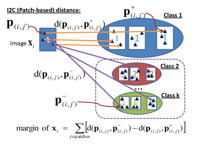
(a) I2C^patch distance

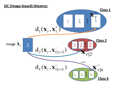
(b) I2C^image distance

Figure 1: Illustration of I2C^patch and I2C^image distances. Here we assume that the image ${\boldsymbol{x}}_{i}$ belongs to class $1$. (a) Patches in the image are represented by black triangles. Each orange arrow maps the patch ${\boldsymbol{p}}_{(i,j^{\prime})}$ to the closest patch with the same class label ${\boldsymbol{p}}_{(i,j^{\prime})}^{+}$. Each purple arrow maps the patch ${\boldsymbol{p}}_{(i,j^{\prime})}$ to the closest patch with the different class label ${\boldsymbol{p}}_{(i,j^{\prime})}^{-}$. To achieve high accuracy, we prefer $d({{\boldsymbol{p}}_{(i,j)}},{{\boldsymbol{p}}_{(i,j)}^{+}})$ to be small and $d({{\boldsymbol{p}}_{(i,j)}},{{\boldsymbol{p}}_{(i,j)}^{-}})$ to be large. Our method learns hash functions that preserve the relative comparison relationships in the data, i.e., the margin of ${\boldsymbol{x}}_{i}$ should be as large as possible. (b) Each image now contains one single patch. Each orange arrow maps the image ${\boldsymbol{x}}_{i}$ to several closest images with the same class label ${\boldsymbol{x}}_{i}^{+}$.

III Approach

In this section, we present the I2C distance definition. We then define our margins and propose two approaches which learn a set of hash functions and their coefficients (weighted Hamming distance). We then discuss the application and computational complexity of the proposed approach.

III-A Background

I2C distance

Suppose we are given a set of training images $\{({\boldsymbol{x}}_{i},y_{i})\}_{i=1}^{m}$ where ${{\boldsymbol{x}}_{i}}\in\mathbb{R}^{d}$ represents a $d$-dimensional image and $y_{i}\in\{1,\cdots,k\}$ the corresponding class label. Here $m$ is the number of training instances and $k$ is the number of classes. Let $\{{\boldsymbol{p}}_{(i,1)},\cdots,{\boldsymbol{p}}_{(i,n)}\}$ denote a collection of local feature descriptors, in which ${{\boldsymbol{p}}_{(i,j)}}$ represents features extracted from the $j$-th patch in the $i$-th image. Here $n$ represents the number of patches in ${{\boldsymbol{x}}_{i}}$ and visual features can simply be its pixel intensity values or local distinct feature descriptors such as SIFT [27], Edge-SIFT [28] or SURF [29]. To calculate the I2C distance from an image ${{\boldsymbol{x}}_{i}}$ to a candidate class $r$, NBNN finds the nearest neighbour to each feature ${{\boldsymbol{p}}_{(i,j)}}$ from each class $r$. The I2C distance is defined as the sum of Euclidean distances between each feature ${{\boldsymbol{p}}_{(i,j)}}$ in image ${{\boldsymbol{x}}_{i}}$ and its nearest neighbour from class $r$, ${\rm NN}_{r}({{\boldsymbol{p}}_{(i,j)}})$. The distance can be written as [18]: $\sum_{j=1}^{n}\|{{\boldsymbol{p}}_{(i,j)}}-{\rm NN}_{r}({{\boldsymbol{p}}_{(i,j)}})\|^{2}$. The NBNN classifier is of the form

$$F({{\boldsymbol{x}}_{i}})=\mathop{\mathrm{argmin}}\limits_{r=1,\cdots,k}\sum_{j=1}^{n}\|{{\boldsymbol{p}}_{(i,j)}}-{\rm NN}_{r}({{\boldsymbol{p}}_{(i,j)}})\|^{2}$$ (1)

where ${\rm NN}_{r}({{\boldsymbol{p}}_{(i,j)}})$ is the nearest neighbour patch of ${{\boldsymbol{p}}_{(i,j)}}$ in class $r$.

Patch-based I2C margin

The objective of this paper is to learn a set of compact and highly discriminative binary codes $\{h_{1}(\cdot),\ldots,h_{t}(\cdot)\}$, $\in\cal{H}$, each of which maps the patch ${{\boldsymbol{p}}_{(i,j)}}$ into the binary space $\{-1,+1\}$. The I2C margin is based on the I2C distance proposed for the NBNN classifier. To better model a pair-wise proximity, we define the weighted distance between any two input patches, ${\boldsymbol{p}}$ and ${{\boldsymbol{p}}^{\prime}}$ as $d({\boldsymbol{p}},{{\boldsymbol{p}}^{\prime}})=\sum_{s=1}^{t}w_{s}|h_{s}({\boldsymbol{p}})-h_{s}({{\boldsymbol{p}}^{\prime}})|$. Here ${\boldsymbol{w}}=\left[w_{1},\cdots,w_{t}\right]\in\mathbb{R}^{t}$ is the (non-negative) weight vector. We formulate the I2C margin of the $i$-th image based on the intuition that the distance of patch ${{\boldsymbol{p}}_{(i,j)}}$ to any other classes (${{\boldsymbol{p}}_{(i,j)}^{-}}$) should be larger than the distance to its belonging class (${{\boldsymbol{p}}_{(i,j)}^{+}}$). The I2C^patch margin can be written as,

$$\varrho_{i} =\sum_{j=1}^{n}\left[d({{\boldsymbol{p}}_{(i,j)}},{{\boldsymbol{p}}_{(i,j)}^{-}})-d({{\boldsymbol{p}}_{(i,j)}},{{\boldsymbol{p}}_{(i,j)}^{+}})\right]$$ (2)

$$=\left(\textstyle\sum_{j}{\boldsymbol{a}}_{(i,j)}\right){\boldsymbol{w}}$$

where ${{\boldsymbol{p}}_{(i,j)}^{-}}={\rm NN}_{\neq y_{i}}({{\boldsymbol{p}}_{(i,j)}})$ is the nearest neighbour patch of ${{\boldsymbol{p}}_{(i,j)}}$ with a different class label (purple arrows in Fig. 1a), ${{\boldsymbol{p}}_{(i,j)}^{+}}={\rm NN}_{y_{i}}({{\boldsymbol{p}}_{(i,j)}})$ is the nearest neighbour patch of ${{\boldsymbol{p}}_{(i,j)}}$ with the same class label (orange arrows in Fig. 1a), ${\boldsymbol{a}}_{(i,j)}=\left[a_{(i,j),1},\cdots,a_{(i,j),t}\right]$, and $a_{(i,j),s}=\bigl{[}|h_{s}({{\boldsymbol{p}}_{(i,j)}})-h_{s}({{\boldsymbol{p}}_{(i,j)}^{-}})|-|h_{s}({{\boldsymbol{p}}_{(i,j)}})-h_{s}({{\boldsymbol{p}}_{(i,j)}^{+}})|\bigr{]}$. We thus aim to learn a set of functions, $\{h_{s}(\cdot)\}_{s=1}^{t}$, where $h({\boldsymbol{p}};{\boldsymbol{\beta}},b)=\operatorname{\bf sign}({\boldsymbol{\beta}}^{\!\top}{\boldsymbol{p}}+b)$, such that the weighted distance between two binary codes $[h_{1}({{\boldsymbol{p}}_{(i,j)}}),\cdots,h_{t}({{\boldsymbol{p}}_{(i,j)}})]$ and $[h_{1}({{\boldsymbol{p}}_{(i,j)}^{+}}),\cdots,h_{t}({{\boldsymbol{p}}_{(i,j)}^{+}})]$ remains small.

Image-based I2C margin

In this paper, we extend the I2C margin originally designed for key-point matching to image matching. We represent the whole image as a large single patch. Similar to the previous margin, the orange arrow can be mapped to multiple patches (images). We illustrate our new I2C^image in Fig. 1b. We define the new margin based on the intuition that the distance between a pair of irrelevant images (image ${{\boldsymbol{x}}_{\tau}}$ and images from any other classes) should be larger than the distance between a pair of relevant images (image ${{\boldsymbol{x}}_{\tau}}$ and images from its belonging class). The training data can be written in a form of triplets $\{({{\boldsymbol{x}}_{\tau}},{{\boldsymbol{x}}_{{\tau}}^{+}},{{\boldsymbol{x}}_{{\tau}|r}^{-}})\}_{{\tau}=1}^{|\mathcal{S}|}$ where each triplet indicates the relationship of three images, $\mathcal{S}$ is the triplet index set and $|\mathcal{S}|$ is the total number of triplets. Here ${{\boldsymbol{x}}_{{\tau}}^{+}}$ is a set of nearest neighbours from the same class and ${{\boldsymbol{x}}_{{\tau}|r}^{-}}$ is a set of nearest neighbours from class $r$ ($r\neq{y_{{\tau}}}$). Unlike the I2C^patch distance, we parameterized each class by a weight vector associated with the class label. Since we have $k$ classes, we define the matrix ${\boldsymbol{W}}=[{\boldsymbol{w}}_{1},\cdots,{\boldsymbol{w}}_{k}]$, such that the $r$-th column of ${\boldsymbol{W}}$ contains Hamming weights for class $r$. The weighted Hamming distance between any two data points, ${{\boldsymbol{x}}_{i}}$ and ${\boldsymbol{x}}_{j}$, is defined as $\Delta_{r}({{\boldsymbol{x}}_{i}},{\boldsymbol{x}}_{j})=\sum_{s=1}^{t}w_{s,r}|h_{s}({{\boldsymbol{x}}_{i}})-h_{s}({\boldsymbol{x}}_{j})|$. Here $\left[w_{1,r},\cdots,w_{t,r}\right]\in\mathbb{R}^{t}$ is the (non-negative) weight vector associated with the class label $r$. We define the margin for ${{\boldsymbol{x}}_{\tau}}$ as the difference between two distances (i) weighted distance between ${{\boldsymbol{x}}_{\tau}}$ and ${{\boldsymbol{x}}_{{\tau}|r}^{-}}$, and (ii) weighted distance between ${{\boldsymbol{x}}_{\tau}}$ and ${{\boldsymbol{x}}_{{\tau}}^{+}}$:

$$\rho_{{\tau},r} =\Delta({{\boldsymbol{x}}_{\tau}},{{\boldsymbol{x}}_{{\tau}|r}^{-}})-\Delta({{\boldsymbol{x}}_{\tau}},{{\boldsymbol{x}}_{{\tau}}^{+}})$$ (3)

$$={{\boldsymbol{a}}_{({\tau}|r)}}{\boldsymbol{w}}_{{y_{{\tau}}}}-{{\boldsymbol{a}}_{({\tau}|r)}}{\boldsymbol{w}}_{r}$$

where ${\tau}$ is an index of the triplet set $\{({{\boldsymbol{x}}_{\tau}},{{\boldsymbol{x}}_{{\tau}}^{+}},{{\boldsymbol{x}}_{{\tau}|r}^{-}})\}_{{\tau}=1}^{\mathcal{|S|}}$, ${{\boldsymbol{a}}_{({\tau}|r)}}=\left[a_{({\tau}|r),1},\cdots,a_{({\tau}|r),t}\right]$, and $a_{({\tau}|r),s}=\bigl{[}|h_{s}({{\boldsymbol{x}}_{\tau}})-h_{s}({{\boldsymbol{x}}_{{\tau}|r}^{-}})|-|h_{s}({{\boldsymbol{x}}_{\tau}})-h_{s}({{\boldsymbol{x}}_{{\tau}}^{+}})|\bigr{]}$. Similar to the patch-based approach, we thus aim to learn a set of functions, $\{h_{s}(\cdot)\}_{s=1}^{t}$, where $h({\boldsymbol{x}};{\boldsymbol{\beta}},b)=\operatorname{\bf sign}({\boldsymbol{\beta}}^{\!\top}{\boldsymbol{x}}+b)$.

III-B Learning compact descriptors

In this section, we design the new approach using the large margin framework. The optimization problem is formulated such that the distance of the nearest instance from the same class (nearest hit) is smaller than the distance of the nearest instance from other classes (nearest miss).

Patch-based I2C optimization

The general $\ell_{1}$-regularized optimization problem for the patch-based I2C margin is

$$\min_{{\boldsymbol{w}},{\boldsymbol{\varrho}}}\; {\textstyle\sum}_{i=1}^{m}L(\varrho_{i})+\nu\|{\boldsymbol{w}}\|_{1}$$ (4)

$$\mathop{\mathrm{s.t.\!\!:}}\nolimits\; \varrho_{i}=\left({\textstyle\sum}_{j}{\boldsymbol{a}}_{(i,j)}\right){\boldsymbol{w}},\forall i,j;\;{\boldsymbol{w}}\geq 0,$$

where $L$ can be any convex loss function, the regularization parameter $\nu$ determines the trade-off between the data-fitting loss function and the model complexity, subscripts $i$ and $j$ index images and patches, respectively. Here we introduce the auxiliary variables, ${\boldsymbol{\varrho}}$, to obtain a meaningful dual formulation. For the logistic loss, the learning problem can be expressed as:

$$\min_{{\boldsymbol{w}},{\boldsymbol{\varrho}}}\; {\textstyle\sum}_{i}\log\left(1+\exp(-\varrho_{i})\right)+\nu\|{\boldsymbol{w}}\|_{1}$$ (5)

$$\mathop{\mathrm{s.t.\!\!:}}\nolimits\; \varrho_{i}=\left({\textstyle\sum}_{j}{\boldsymbol{a}}_{(i,j)}\right){\boldsymbol{w}},\forall i,j;\;{\boldsymbol{w}}\geq 0,$$

The Lagrangian of (5) can be written as:

$${\varLambda}\; =\sum_{i}\log(1+\exp(-\varrho_{i}))+\nu{\boldsymbol{1}}^{\!\top}{\boldsymbol{w}}$$

$$\quad-\sum_{i}v_{i}\left(\varrho_{i}-\left({\textstyle\sum}_{j}{\boldsymbol{a}}_{(i,j)}\right){\boldsymbol{w}}\right)-{\boldsymbol{q}}^{\!\top}{\boldsymbol{w}},$$

with ${\boldsymbol{q}}\geq 0$. The dual function is:

$$\inf_{{\boldsymbol{w}},{\boldsymbol{\varrho}}}{\varLambda}\; =\inf_{{\boldsymbol{w}},{\boldsymbol{\varrho}}}{\textstyle\sum}_{i}\log(1+\exp(-\varrho_{i}))-{\textstyle\sum}_{i}v_{i}\varrho_{i}$$

$$\quad\quad+\overbrace{\bigl{(}{\textstyle\sum}_{i}v_{i}({\textstyle\sum}_{j}{\boldsymbol{a}}_{(i,j)})-{\boldsymbol{q}}^{\!\top}+\nu{\boldsymbol{1}}^{\!\top}\bigr{)}}^{\text{must be zero}}{\boldsymbol{w}}.$$

Since the convex conjugate function of the logistic loss, $\log\left(1+\exp(-x)\right)$, is $(-u)\log(-u)+(1+u)\log(1+u)$ if $-1\leq u\leq 0$ and $\infty$ otherwise. The Lagrange dual for the logistic loss is:

$$\max_{{\boldsymbol{v}}} -{\textstyle\sum}_{i=1}^{m}\Bigl{[}-v_{i}\log(-v_{i})+(1+v_{i})\log(1+v_{i})\Bigr{]}$$

$$\mathop{\mathrm{s.t.\!\!:}}\nolimits\; {\textstyle\sum}_{i=1}^{m}v_{i}\left({\textstyle\sum}_{j}{\boldsymbol{a}}_{(i,j)}\right)\geq-\nu{\boldsymbol{1}}^{\!\top},\;{\boldsymbol{v}}\geq 0.$$

By reversing the sing of ${\boldsymbol{v}}$, we obtain:

$$\min_{{\boldsymbol{v}}} {\textstyle\sum}_{i=1}^{m}\Bigl{[}v_{i}\log(v_{i})+(1-v_{i})\log(1-v_{i})\Bigr{]}$$ (6)

$$\mathop{\mathrm{s.t.\!\!:}}\nolimits\; {\textstyle\sum}_{i=1}^{m}v_{i}\left({\textstyle\sum}_{j}{\boldsymbol{a}}_{(i,j)}\right)\leq\nu{\boldsymbol{1}}^{\!\top},\;{\boldsymbol{v}}\geq 0.$$

Image-based I2C optimization

The general $\ell_{1}$-regularized optimization problem we want to solve is

$$\min_{{\boldsymbol{W}},{\boldsymbol{\rho}}}\; {\textstyle\sum}_{{\tau},r}L(\rho_{{\tau},r})+\nu\|{\boldsymbol{W}}\|_{1}$$ (7)

$$\mathop{\mathrm{s.t.\!\!:}}\nolimits\; \rho_{{\tau},r}={{\boldsymbol{a}}_{({\tau}|r)}}{\boldsymbol{w}}_{{y_{{\tau}}}}-{{\boldsymbol{a}}_{({\tau}|r)}}{\boldsymbol{w}}_{r},\forall{\tau},r;\;{\boldsymbol{W}}\geq 0.$$

The learning problem for the logistic loss can be expressed as:

$$\min_{{\boldsymbol{W}},{\boldsymbol{\rho}}}\; {\textstyle\sum}_{{\tau},r}\log\left(1+\exp(-\rho_{{\tau},r})\right)+\nu\|{\boldsymbol{W}}\|_{1}$$ (8)

$$\mathop{\mathrm{s.t.\!\!:}}\nolimits\; \rho_{{\tau},r}={{\boldsymbol{a}}_{({\tau}|r)}}{\boldsymbol{w}}_{{y_{{\tau}}}}-{{\boldsymbol{a}}_{({\tau}|r)}}{\boldsymbol{w}}_{r},\forall{\tau},r;\;{\boldsymbol{W}}\geq 0.$$

The Lagrangian of (8) can be written as

$${\varLambda}( {\boldsymbol{W}},{\boldsymbol{\rho}},{\boldsymbol{U}},{\boldsymbol{Z}})\;={\textstyle\sum}_{{\tau},r}\log(1+\exp(-\rho_{{\tau},r}))+\nu{\textstyle\sum}_{r}{\boldsymbol{w}}_{r}$$

$$-{\textstyle\sum}_{{\tau},r}u_{{\tau},r}(\rho_{{\tau},r}-{{\boldsymbol{a}}_{({\tau}|r)}}{\boldsymbol{w}}_{{y_{{\tau}}}}+{{\boldsymbol{a}}_{({\tau}|r)}}{\boldsymbol{w}}_{r})-\operatorname{\bf Tr}({\boldsymbol{Z}}^{\!\top}{\boldsymbol{W}}),$$

with ${\boldsymbol{Z}}\geq 0$. The Lagrangian function is

$$\inf_{{\boldsymbol{W}},{\boldsymbol{\rho}}}{\varLambda}( {\boldsymbol{W}},{\boldsymbol{\rho}},{\boldsymbol{U}},{\boldsymbol{Z}})$$ (9)

$$= -{\textstyle\sum}_{{\tau},r}\sup_{\rho_{{\tau},r}}\Bigl{(}u_{{\tau},r}\rho_{{\tau},r}-\log(1+\exp(-\rho_{{\tau},r}))\Bigr{)}$$

$$\quad+\inf_{{\boldsymbol{W}}}\Bigl{(}\nu{\textstyle\sum}_{r}{\boldsymbol{w}}_{r}+{\textstyle\sum}_{{\tau},r}u_{{\tau},r}{{\boldsymbol{a}}_{({\tau}|r)}}{\boldsymbol{w}}_{{y_{{\tau}}}}$$

$$\quad\quad\quad-{\textstyle\sum}_{{\tau},r}u_{{\tau},r}{{\boldsymbol{a}}_{({\tau}|r)}}{\boldsymbol{w}}_{r}-\operatorname{\bf Tr}({\boldsymbol{Z}}^{\!\top}{\boldsymbol{W}})\Bigr{)}.$$

At optimum the first derivative of the Lagrangian with respect to each row of ${\boldsymbol{W}}$ must be zeros, i.e., $\frac{\partial{\varLambda}}{\partial{\boldsymbol{w}}_{r}}={\bf 0}$, and therefore

$$\;\sum_{{\tau}\mid{y_{{\tau}}}=r} \left(\textstyle\sum_{l}u_{{\tau},l}\right){{\boldsymbol{a}}_{({\tau}|r)}}-\sum_{{\tau}}u_{{\tau},r}{{\boldsymbol{a}}_{({\tau}|r)}}={\boldsymbol{z}}_{r:}-\nu{\boldsymbol{1}}^{\!\top}$$

$$\Rightarrow{\textstyle\sum}_{{\tau}}\delta_{r,{y_{{\tau}}}}\left(\textstyle\sum_{l}u_{{\tau},l}\right){{\boldsymbol{a}}_{({\tau}|r)}}-{\textstyle\sum}_{{\tau}}u_{{\tau},r}{{\boldsymbol{a}}_{({\tau}|r)}}\geq-\nu{\boldsymbol{1}}^{\!\top},$$

$\forall r$ and $\delta_{s,t}=1$ if $s=t$ and $0$, otherwise. The Lagrange dual problem is

$$\max_{{\boldsymbol{U}}}\quad -{\textstyle\sum}_{{\tau},r}\Bigl{[}-u_{{\tau},r}\log\left(-u_{{\tau},r}\right)+\left(1+u_{{\tau},r}\right)\log\left(1+u_{{\tau},r}\right)\Bigr{]}$$

$$\mathop{\mathrm{s.t.\!\!:}}\nolimits\quad {\textstyle\sum}_{{\tau}}\left[\delta_{r,{y_{{\tau}}}}(\textstyle\sum_{l}u_{{\tau},l})-u_{{\tau},r}\right]{{\boldsymbol{a}}_{({\tau}|r)}}\geq-\nu{\boldsymbol{1}}^{\!\top},\forall r;$$

By reversing the sign of ${\boldsymbol{U}}$, we obtain

$$\min_{{\boldsymbol{U}}}\quad {\textstyle\sum}_{{\tau},r}\Bigl{[}u_{{\tau},r}\log\left(u_{{\tau},r}\right)+\left(1-u_{{\tau},r}\right)\log\left(1-u_{{\tau},r}\right)\Bigr{]}$$

$$\mathop{\mathrm{s.t.\!\!:}}\nolimits\quad {\textstyle\sum}_{{\tau}}\left[\delta_{r,{y_{{\tau}}}}(\textstyle\sum_{l}u_{{\tau},l})-u_{{\tau},r}\right]{{\boldsymbol{a}}_{({\tau}|r)}}\leq\nu{\boldsymbol{1}}^{\!\top},\forall r;$$ (10)

General convex loss

In this section, we generalize our approach to any convex losses with $\ell_{1}$-norm penalty. Note that our approach is not limited to the $\ell_{1}$-norm regularized framework but other $\ell_{p}$-norm penalties ($p>1$) can also be applied (see the Appendix). The Lagrangian of (7) can be written as:

$${\varLambda}={\textstyle\sum}_{{\tau},r} L(\rho_{{\tau},r})+\nu{\textstyle\sum}_{r}{\boldsymbol{w}}_{r}-{\textstyle\sum}_{{\tau},r}u_{{\tau},r}$$

$$(\rho_{{\tau},r}-{{\boldsymbol{a}}_{({\tau}|r)}}{\boldsymbol{w}}_{{y_{{\tau}}}}+{{\boldsymbol{a}}_{({\tau}|r)}}{\boldsymbol{w}}_{r})-\operatorname{\bf Tr}({\boldsymbol{Z}}^{\!\top}{\boldsymbol{W}}),$$

with ${\boldsymbol{Z}}\geq 0$. Following our derivation for the logistic loss, the Lagrange dual can be written as

$$\min_{{\boldsymbol{U}},{\boldsymbol{Q}}}\quad {\textstyle\sum}_{{\tau},r}L^{\ast}(-u_{{\tau},r})$$ (11)

$$\mathop{\mathrm{s.t.\!\!:}}\nolimits\quad {\textstyle\sum}_{{\tau}}\left[\delta_{r,{y_{{\tau}}}}(\textstyle\sum_{l}u_{{\tau},l})-u_{{\tau},r}\right]{{\boldsymbol{a}}_{({\tau}|r)}}\leq\nu{\boldsymbol{1}}^{\!\top},\forall r;$$

where $L^{\ast}(\cdot)$ is the Fenchel dual function of $L(\cdot)$. Through the KKT optimality condition, the duality gap between the solutions of the primal optimization problem (7) and the dual problem (11) must coincide since both problems are feasible and the Slater’s condition is satisfied. The required relationship between the optimal values of ${\boldsymbol{U}}$ and ${\boldsymbol{\rho}}$ (for I2C^image) and between the optimal values of ${\boldsymbol{v}}$ and ${\boldsymbol{\varrho}}$ (for I2C^patch) thus hold at optimality. These relationships can be expressed as $u_{{\tau},r}=-L^{\prime}(\rho_{{\tau},r})$ (for I2C^image) and $v_{i}=-L^{\prime}(\varrho_{i})$ (for I2C^patch). For the logistic loss of (7) and (4), we can write these relationships as:

$$u_{{\tau},r}^{\ast}=\frac{\exp(-\rho_{{\tau},r}^{\ast})}{1+\exp(-\rho_{{\tau},r}^{\ast})}$$ (12)

and

$$v_{i}^{\ast}=\frac{\exp(-\varrho_{i}^{\ast})}{1+\exp(-\varrho_{i}^{\ast})},$$ (13)

respectively.

Learning binary output functions

Since there may be infinitely many constraints in (11), we use column generation to identify an optimal set of constraints [4]. Column generation allows us to avoid solving the original problem, which has a large number of constraints, and instead to consider a much smaller problem which guarantees the new solution to be optimal for the original problem. The algorithm begins by finding the most violated dual constraint in the dual problem (11) and inserts this constraint into the new optimization problem (which corresponds to inserting a primal variable). From (11) the subproblem for generating the most violated dual constraint, $h^{\ast}(\cdot)$, is

$$h^{\ast}(\cdot)=\mathop{\mathrm{argmax}}\limits_{h(\cdot)\in\mathcal{H},r}\;{\textstyle\sum}_{{\tau}}(\delta_{r,{y_{{\tau}}}}(\textstyle\sum_{l}u_{{\tau},l})-u_{{\tau},r}){a_{({\tau}|r)}},$$ (14)

where ${a_{({\tau}|r)}}=|h({{\boldsymbol{x}}_{\tau}})-h({{\boldsymbol{x}}_{{\tau}|r}^{-}})|-|h({{\boldsymbol{x}}_{\tau}})-h({{\boldsymbol{x}}_{{\tau}}^{+}})|$ and $h({{\boldsymbol{x}}_{i}})=\operatorname{\bf sign}({\boldsymbol{\beta}}^{\!\top}{{\boldsymbol{x}}_{i}}+b)$. At each iteration, we thus add an additional constraint to the dual problem. The process continues until there are no violated constraints or the maximum number of iterations is reached.

Not only (14) is non-convex but also exhaustively evaluating all possible candidates in the hypothesis space is infeasible. We thus treat the problem of learning binary output functions as the gradient ascent optimization problem. To achieve this, we replace $|\cdot|$ and $\operatorname{\bf sign}(\cdot)$ operators in (14) with $(\cdot)^{2}$ and $\frac{2}{\pi}\arctan(\cdot)$, respectively, due to their differentiability. Note that it is possible to replace $\operatorname{\bf sign}(\cdot)$ with other sigmoid functions, e.g., $\frac{1}{1+\exp(-t)}$. We used $\arctan(\cdot)$ here as it has been successfully applied to learn features in [34]. To summarize, we replace $a_{({\tau})}$ and $h({{\boldsymbol{x}}_{\tau}};{\boldsymbol{\beta}},b)$ in (14) with,

$$a_{({\tau})}\rightarrow\bigl{(}h({{\boldsymbol{x}}_{\tau}})-h({{\boldsymbol{x}}_{{\tau}|r}^{-}})\bigr{)}^{2}- \bigl{(}h({{\boldsymbol{x}}_{\tau}})-h({{\boldsymbol{x}}_{{\tau}}^{+}})\bigr{)}^{2},$$

$$h({{\boldsymbol{x}}_{\tau}};{\boldsymbol{\beta}},b)\rightarrow\frac{2}{\pi} \arctan({\boldsymbol{\beta}}^{\!\top}{{\boldsymbol{x}}_{\tau}}+b).$$

Given an initial value of $({\boldsymbol{\beta}},b)$, we iteratively search for the new value that leads to the larger value of $\sum_{{\tau}}(\delta_{r,{y_{{\tau}}}}(\textstyle\sum_{l}u_{{\tau},l})-u_{{\tau},r}){a_{({\tau}|r)}}$ based on the gradient ascent method. To find a local maximum, we repeatedly take a step proportional to the gradient of the function at the current point. The iteration stops when the magnitude of the gradient is smaller than some threshold, i.e., the objective value is at its local maximum.

For ease of exposition, we define the following variables: ${{{{\tilde{h}}}}_{\tau}}=h({{\boldsymbol{x}}_{\tau}})$, ${{{{\tilde{h}}}}^{+}_{\tau}}=h({{\boldsymbol{x}}_{{\tau}}^{+}})$, ${{{{\tilde{h}}}}^{-}_{\tau}}=h({{\boldsymbol{x}}_{{\tau}|r}^{-}})$ and $\omega_{({\tau},r)}=(\delta_{r,{y_{{\tau}}}}(\textstyle\sum_{l}u_{{\tau},l})-u_{{\tau},r})$. Let $\Pi=\sum_{{\tau}}(\delta_{r,{y_{{\tau}}}}(\textstyle\sum_{l}u_{{\tau},l})-u_{{\tau},r}){a_{({\tau}|r)}}$. The gradient of $\Pi$ can then be expressed as:

$$\frac{\partial\Pi}{\partial{\boldsymbol{\beta}}} ={\textstyle\sum}_{{\tau}}\omega_{({\tau},r)}\frac{\partial{a_{({\tau}|r)}}}{\partial{\boldsymbol{\beta}}},$$ (15)

$$\frac{\partial\Pi}{\partial b} ={\textstyle\sum}_{{\tau}}\omega_{({\tau},r)}\frac{\partial{a_{({\tau}|r)}}}{\partial b},$$ (16)

where

$$\frac{\partial{a_{({\tau}|r)}}}{\partial{\boldsymbol{\beta}}} =2({{{{\tilde{h}}}}_{\tau}}-{{{{\tilde{h}}}}^{-}_{\tau}})\left(\frac{\partial{{{{\tilde{h}}}}_{\tau}}}{\partial{\boldsymbol{\beta}}}-\frac{\partial{{{{\tilde{h}}}}^{-}_{\tau}}}{\partial{\boldsymbol{\beta}}}\right)$$

$$\quad-2({{{{\tilde{h}}}}_{\tau}}-{{{{\tilde{h}}}}^{+}_{\tau}})\left(\frac{\partial{{{{\tilde{h}}}}_{\tau}}}{\partial{\boldsymbol{\beta}}}-\frac{\partial{{{{\tilde{h}}}}^{+}_{\tau}}}{\partial{\boldsymbol{\beta}}}\right),$$

$$\frac{\partial{{{{\tilde{h}}}}_{\tau}}}{\partial{\boldsymbol{\beta}}} =\frac{2}{\pi}\frac{{{\boldsymbol{x}}_{\tau}}}{1+({\boldsymbol{\beta}}^{\!\top}{{\boldsymbol{x}}_{\tau}}+b)^{2}},$$

$$\frac{\partial{a_{({\tau}|r)}}}{\partial b} =2({{{{\tilde{h}}}}_{\tau}}-{{{{\tilde{h}}}}^{-}_{\tau}})\left(\frac{\partial{{{{\tilde{h}}}}_{\tau}}}{\partial b}-\frac{\partial{{{{\tilde{h}}}}^{-}_{\tau}}}{\partial b}\right)$$

$$\quad-2({{{{\tilde{h}}}}_{\tau}}-{{{{\tilde{h}}}}^{+}_{\tau}})\left(\frac{\partial{{{{\tilde{h}}}}_{\tau}}}{\partial{\boldsymbol{\beta}}}-\frac{\partial{{{{\tilde{h}}}}^{+}_{\tau}}}{\partial{\boldsymbol{\beta}}}\right),$$

$$\frac{\partial{{{{\tilde{h}}}}_{\tau}}}{\partial b} =\frac{2}{\pi}\frac{1}{1+({\boldsymbol{\beta}}^{\!\top}{{\boldsymbol{x}}_{\tau}}+b)^{2}}.$$

Since using a fixed small learning rate can yield a poor convergence, a more sophisticated off-the-shelf optimization method can be a better alternative. In our implementation, we use a limited memory BFGS (L-BFGS) [35] to perform a line search algorithm. At each L-BFGS iteration, we use (15) and (16) to compute the search direction. Since (14) is highly non-convex, choosing the initial value of $({\boldsymbol{\beta}},b)$ is critical to finding the global maximum. We randomly generate a large number of $({\boldsymbol{\beta}},b)$ pairs and use the pair with the highest response as an initial value for L-BFGS. Note that the same solver has also been used to speed up training in deep learning [36].

Algorithm 1 Training algorithm for I2C^patch C-BID.

Learning Hamming weights

Hamming weights can be calculated in a totally corrective manner as in [4]. For the logistic loss formulation, the primal problem has $tk$ variables and $\mathcal{|S|}$ constraints. Here $|\cdot|$ counts the number of elements in the triplet set. Since the scale of the primal problem is much smaller than the dual problem, we solve the primal problem instead of the dual problem. The primal problem, (7), can be solved using an efficient Quasi-Newton method like L-BFGS-B, and the dual variables can be obtained using the KKT condition, (12) and (13). The details of our I2C^patch and I2C^image C-BID algorithms are given in Algorithm LABEL:ALG:alg_patch and LABEL:ALG:alg_image, respectively.

Algorithm 2 Training algorithm for I2C^image C-BID.

III-C Application

In this section, we illustrate how the proposed compact binary code can be applied to the image classification problem using both I2C^patch and I2C^image approaches.

Patch-based I2C approach

In NBNN the training data for a class is a collection of small patches densely extracted from given training images[18]. Since the dimension of visual descriptors is large and patches are sampled densely, the storage space and the retrieval time are two critical issues that need to be addressed. In this section, we illustrate how our approach can be applied to reduce the storage space and improve the retrieval time. Following NBNN, we first extract a large number of visual patches from each training image at the same orientation but multiple spatial scales. During training, each patch is mapped to have the same binary code as the most similar patch from the same class. During evaluation, a large number of patches are extracted from the test image and the label is assigned based on the minimal distance between test patches and training patches, i.e., $\mathop{\mathrm{argmin}}\limits_{\ell}\,\sum_{j=1}^{n}\sum_{s=1}^{t}w_{s}|h_{s}({\boldsymbol{p}}_{j})-h_{s}({\boldsymbol{p}}_{j+})|$, where $n$ is the total number of patches in the image and ${\boldsymbol{p}}_{j+}$ represents the training patch from class $\ell$ such that $d\bigl{(}[h_{1}({\boldsymbol{p}}_{j}),\cdots,h_{t}({\boldsymbol{p}}_{j})],[h_{1}({\boldsymbol{p}}_{j+}),\cdots,h_{t}({\boldsymbol{p}}_{j+})]\bigr{)}$ $=\sum_{s=1}^{t}w_{s}|h_{s}({\boldsymbol{p}}_{j})-h_{s}({\boldsymbol{p}}_{j+})|$ is minimal. Note that, in order to further improve the efficiency during retrieval, binary outputs of the training data, i.e., $\{h_{s}({{\boldsymbol{p}}_{(i,j)}})\}_{s=1}^{t}$, $i=1,\cdots,m$, $j=1,\cdots,n$, can be pre-computed offline. The details of our C-BID classifier for patch-based I2C distance are given in Algorithm LABEL:ALG:alg3.

Algorithm 3 I2C^patch C-BID classifier.

Image-based I2C approach

The typical steps involved in the image-based model are: (i) feature extraction (ii) learning a multi-class classifier. Our algorithm falls in between step (i) and (ii). In other words, we represent the output of step (i) in a more compact form. The new descriptor significantly reduces the storage space required while preserving pair-wise distances between the input data.

III-D Computational complexity

During training (offline), we need to iteratively find the best hash function (14) and solve the primal problem (7). The computational complexity during training is similar to LPBoost [4]. During evaluation (online), the time complexity is almost the same as other hashing algorithms. With a proper implementation, weighted hamming distance can be calculated almost as fast as hamming distance. For example, one can use the hamming distance to retrieve similar items. Retrieved items can be re-ranked using hamming weights. To further improve the speed, the weighted hamming distance between $8$ consecutive bits of the query and binary codes can be pre-computed and stored in a lookup table [37]. In addition, vector multiplication can be computed efficiently using a linear algebra library.

IV Experiments

We evaluate the proposed C-BID on both synthetic data set and computer vision tasks. Unless otherwise specified, we use the logistic loss with $\ell_{1}$-norm penalty.

IV-A Patch-based I2C distance

In this section, we perform experiments using our C-BID with NBNN based approach. All images are resized to a maximum of $150\times 150$ pixels prior to processing. We use dense SIFT features in all algorithms. We randomly select $10$ images per class as the training set and $25$ images per class as the test set. All experiments are repeated $5$ times and the average accuracy reported. For Caltech-101, we use five classes similar to [23]: faces, airplanes, cars-side, motorbikes and background. In this experiment, we use $1$ nearest neighbour from the same class and one nearest neighbour from each other classes. We compare our approach with BoW with an additive kernel Map of [38], the original NBNN with SIFT features [18], NBNN with an approximate NN (ANN) search using best-bin first search of kd-tree, NBNN with LSH, and NBNN with SIFT (PCA) features and report experimental results in Table I. From the table, our approach consistently outperforms all NBNN-like approaches and performs best on average. We suspect that the performance improvement of C-BID is due to the large margin learning and the introducing of non-linear functions into the original SIFT descriptor. From the table, our algorithm at $128$ bits consistently performs better than SIFT (PCA) at $512$ bits. From the same table, ANN search tradeoffs speed over accuracy.

Storage

For BoW, we divide an image into $20$ sub-images and the number of visual words is $600$. Hence there are $36,000$ dimensional features being extracted from each image. We also map each feature vector to a higher-dimensional feature space via an explicit map: $\mathbb{R}^{n}\rightarrow\mathbb{R}^{n(2r+1)}$ where $r$ is set to $1$ [38]. Each descriptor is stored as a floating point ($32$ bits), each image requires approximately $141$ kB of storage.

For NBNN, we extract dense SIFT at $4$ different scales. Assuming that a total of $10,000$ SIFT features are extracted and kept in the database from each image (as a $32$-bit floating point representation), NBNN requires approximately $5,000$ kB of storage per image. Using our approach with $32$ binary output functions, the original $128$ dimensional SIFT descriptor ($512$ bytes) is now reduced to $4$ bytes (a $128$-fold reduction in storage) and each image now takes up approximately $39$ kB of storage.

Our approach is also much more efficient than the original NBNN due to its compact binary codes and the use of bitwise exclusive-or operation. Since ANN algorithms, e.g., best bin first and LSH, only index the data, original data points still need to be kept in order to determine the exact distance between the query patch and patches kept in the database. Hence the storage of ANN is similar to that of the exact NN.

Evaluation time

We also report the average evaluation time of various NBNN based approaches (excluding feature extraction time and index building time) in the last row of Table I. Our approach has a much lower evaluation time than the original NBNN with SIFT due to more compact binary codes and the use of bitwise exclusive-or operation. For LSH, we set the number of hash functions per hash table to $20$. We use $25$ hash tables. Hence there are a total of $500$ hash functions ($500$ binary descriptors). However, LSH has a much higher evaluation time than our approach. We suspect that most of the evaluation time is spent in calculating the distance between training samples that are mapped to the same hash bucket, i.e., hash collision.

TABLE I: Experiments on patch-based I2C distance. Performance comparison between BoW + kernel map + SVM [38], SIFT + NBNN [18], SIFT + NBNN + kd-tree search, SIFT + NBNN + LSH, SIFT (PCA) + NBNN and our approach on various data sets. The average accuracy and standard deviation (in percentage) are reported. The last row reports the average evaluation time per image per class of NBNN based approaches (excluding feature extraction time). Experiments are executed on a single core of Intel Core i$7$ $930$ ($2.8$ GHz) with $12$ GB memory. Our approach achieves the higest average accuracy while having a much lower storage cost and evaluation time.

	BoW +	NBNN	NBNN	NBNN	NBNN + SIFT (PCA)		C-BID
	Kernel Map	Exact NN	Best bin first	LSH	$256$	$512$ bits	$16$	$32$	$128$ bits
Graz-02	$70.67$ ($5.7$)	$70.40$ ($7.9$)	$67.47$ ($6.0$)	$62.93$ ($5.3$)	$66.13$ ($6.6$)	$68.80$ ($8.3$)	$65.87$ ($11.4$)	$67.73$ ($9.4$)	$\mathbf{72.27}$ ($\mathbf{7.4}$)
Caltech-101	$\mathbf{86.88}$ ($\mathbf{2.2}$)	$84.96$ ($4.0$)	$84.64$ ($3.9$)	$84.80$ ($3.0$)	$74.72$ ($3.6$)	$83.04$ ($4.9$)	$73.12$ ($7.0$)	$80.96$ ($4.8$)	$86.24$ ($4.2$)
Sports-8	$57.40$ ($3.1$)	$62.20$ ($3.4$)	$59.60$ ($4.1$)	$51.70$ ($3.6$)	$48.40$ ($5.2$)	$54.70$ ($3.9$)	$42.70$ ($3.4$)	$56.90$ ($3.4$)	$\mathbf{63.00}$ ($\mathbf{4.3}$)
Scene-15	$55.73$ ($2.4$)	$54.72$ ($2.6$)	$53.97$ ($2.1$)	$40.21$ ($4.7$)	$46.24$ ($2.1$)	$54.67$ ($1.8$)	$30.03$ ($1.9$)	$54.51$ ($1.8$)	$\mathbf{57.28}$ ($\mathbf{2.8}$)
Avg. accuracy	$67.67$	$68.07$	$66.42$	$59.91$	$58.87$	$65.30$	$52.93$	$65.03$	$\mathbf{69.70}$
Storage$/$image	$141.0$ kB	$5,000.0$ kB	$5,000.0$ kB	$5,000.0$ kB	$312.5$ kB	$625.0$ kB	$19.5$ kB	$39.1$ kB	$156.3$ kB
Eval.$/$img$/$class		$78.8$ sec.	$1.55$ sec.	$3.83$ sec.	$5.50$ sec.	$8.62$ sec.	$0.15$ sec.	$0.24$ sec.	$1.11$ sec.

IV-B Image-based I2C distance

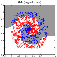
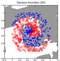
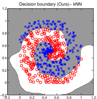
Figure 2: First column: Decision boundary using kNN on a Fermat’s problem ($k=3$). Second column: Decision boundary using kNN on $8$ bits code length learned with Spectral Hashing. Last two columns: Decision boundary using kNN and linear SVM on the $8$ bits feature learned using our approach.

Synthetic data set

We first evaluate the behaviour of C-BID on a Fermat’s problem in which two-class samples are distributed in a two-dimensional space forming a spiral shape. We plot a decision boundary using kNN ($k=3$) and illustrate the result in Fig. 2. We then apply Spectral Hashing (SH) [3] with $8$ bits code length and plot the decision bounding using kNN in the same figure. We observe that SH keeps the neighbourhood relationship of the original data but the decision boundary is not as smooth as the decision boundary of kNN on the original data. We then evaluate our approach by training $8$ bits feature length and plot the decision boundary using two popular classifiers (kNN with $k=3$ and linear SVM). The results are illustrated in the last two columns of Fig. 2. We observe that both classifiers achieve a very similar decision boundary using our features. Compared to the original $2$-D features, which do not exploit class label information, the new feature has a much smoother decision boundary. The results clearly demonstrates the benefit of training visual features using both pair-wise proximity and class-label information.

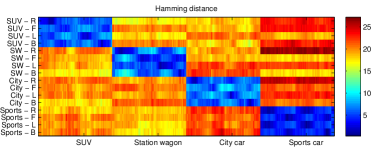
Figure 3: Top: Each class corresponds to each vehicle type (SUV, station wagon (SW), city car and sports car) with orientations ranging from right-profile (R), frontal pose (F), left-profile (L) to back view (B). Bottom: The weighted hamming distance between the binary code of query images and that of the database is illustrated. Each row represents each query image and each column represents each vehicle type being rotated at $4-5$ degrees. Hamming distance can be separated into three groups: a set of training images having the same class and similar orientations to the query image (dark blue), a set of images having the same class but different orientations (light blue), and a set of images having different classes (orange).

Image similarity identification

In this experiment, we demonstrate the capability of C-BID in retrieving similar images to the query image. We use EPFL multi-view car data sets. We categorize vehicles based on their appearance: SUV, station wagon, city car and sports car. Each category consists of the same vehicle type at different poses. For each category, we randomly select $80$ images as the training set and $4$ images, corresponding to the frontal pose, left-profile, right-profile and back view, as the test set. We extract pyramid HOG (pHOG) features and learn C-BID with $256$ bits. The weighted hamming distance between the binary code of test images and the binary code of training images is plotted in Fig. 3. Each row (Fig. 3 Bottom) represents each query image, e.g., SUV-R (the image of SUV captured at the right-profile orientation) is the first query image. Each column represents each vehicle type being rotated at $4-5$ degrees, e.g., the first column represents the image of SUV captured at the right-profile orientation and the second column represents the image of SUV rotated by $5$ degrees from the first column. The binary code learned using C-BID is not only discriminative across different vehicle types but also preserves similarity within the same vehicle category.

Face and pedestrian classification

Next we evaluate the performance of C-BID on face and pedestrian classification. We use $2000$ faces from [41] and randomly extract $2000$ negative patches from background images. We use the original raw pixel intensity and Haar-like features in our experiments. For pedestrians, we use the Daimler-Chrysler pedestrian data sets [42]. We use the original raw pixel intensities and pHOG features. We use $5$ nearest neighbours information per training sample. On both face and pedestrian data sets, C-BID consistently outperforms raw intensity, Haar-like and pHOG features. We show the results of experiments using both Haar-like and pHOG features in Fig. 4.

In the next experiment, we apply C-BID to the baseline pedestrian detector of [43] using INRIA human data sets [43] and TUD-Brussels data sets [44]. INRIA training set consists of $2,416$ cropped mirrored pedestrian images and $1,200$ large background images. The test set contains $288$ images containing $588$ annotated pedestrians and $453$ non-pedestrian images. In this experiment, we only use $288$ images which contain pedestrians [45]. TUD-Brussels test set contains $508$ images containing $1498$ annotated pedestrians. Pedestrian detection is divided into two steps: initial classification and post-verification. The first step is similar to the method described in [43] while, in the second step, we apply C-BID to enforce the pairwise-similarity between positive training samples. To be more specific, in the first step, each training sample is scaled to $64\times 128$ pixels with $16$ pixels additional borders for preserving the contour information. Histogram of oriented gradient features are extracted from $105$ blocks of size $16\times 16$ pixels. Each block is divided into $2\times 2$ cells, and the HOG in each cell is divided into $9$ bins. We train a pedestrian detector using the linear SVM. In the second step, we learn C-BID from HOG extracted in the first step. We use $5$ nearest neighbours information to generate $25$ triplets per positive training image. We learn $3780$ bits descriptor (similar to the original HOG feature length) and build the classifier using the linear SVM. During evaluation, each test image is scanned with $4\times 4$ pixels step size and $10$ scales per octave. For TUD-Brussels, we up-sample the original image to $1280\times 960$ pixels before applying the pedestrian detector. The performance is evaluated using the protocol described in [45]. Both ROC curves are plotted in Fig. 5. We also report the $\log$-average detection rate which is computed by averaging the detection rate at nine FPPI rates evenly spaced in $\log$-space between $10^{-2}$ to $1$. We observe that applying C-BID further improves the $\log$-average detection rate by $5.28\%$ on INRIA test set and $11.87\%$ on TUD-Brussels data sets. This performance gain comes at no additional feature extraction cost. Fig. 9 shows a qualitative assessment of the new detector. We observe that most false positive examples usually contain patterns that mimic the contour of human shoulders or vertical gradients that mimic the torso and leg boundaries.

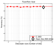
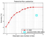
Figure 4: The average face (left) and pedestrian (right) classification performance on various code lengths.

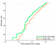
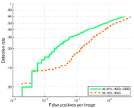
Figure 5: Pedestrian detection performance (left) INRIA (right) TUD-Brussels. Log-average detection rate is also reported.

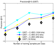
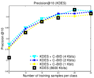
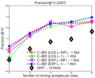
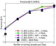
Figure 6: Combining C-BID with GIST and KDES. Top: Average ‘precision rate at $10$’ of different number of training samples per class. Bottom: Average precision rate of logistic and exponential losses with $\ell_{1}$ and $\ell_{\infty}$ penalties. Using GIST, C-BID at $256$ bits consistently outperforms GIST ($512$ dims $\approx$ $16$ kilobits). Using KDES, C-BID at $4096$ bits outperforms KDES ($270,000$ dims $\approx$ $8.6$ megabits).

Combining C-BID with various visual descriptors

Next we evaluate the performance of C-BID using GIST [46] and recently proposed Kernel Descriptors (KDES) [47]. We use UIUC Sports-8 data sets and vary the number of training samples per class. For each split, we train a linear SVM. The results are reported in Fig. 6. We observe that C-BID at $256$ bits consistently outperforms GIST (GIST occupies $4\times 512$ bytes of storage space) and C-BID at $2048$ bits performs comparable to KDES.

In the next experiment, we compare the performance of our binary descriptors with several existing bit-code-based methods. We use the state-of-the-art feature descriptor known as Meta-Class features (MC) [16] to learn binary codes. Experiments are conducted on four different visual data sets: Graz-02, UIUC Sports-8, Scene-15, and Caltech-101. For Graz-02 and Sports-8, we randomly select $50$ images per class for training, $10$ images per class for validation and the remainder for testing. For Scene-15, we randomly select $100$ images for training, $10$ images for validation, and the remainder for testing. For Caltech-101, we randomly select $15$ images per class for training, $5$ images per class for validation, and $20$ images per class for test. We evaluate our algorithm using two different classifiers: K-NN and SVM.

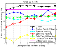
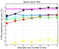
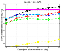
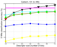
Figure 7: The average k-NN classification performance. We compare our approach with Anchor Graph [10], Spectral Hashing [3], Spherical Hashing [11], Self-Taught Hashing [48], and Laplacian Co-Hashing [49]. The performance of kNN is also plotted. C-BID outperforms all hashing methods as the number of bits increases.

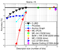
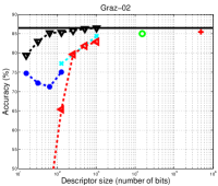
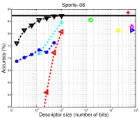
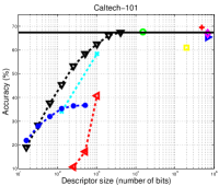
Figure 8: Image classification accuracy on Scene-15, Graz-02, Sports-8 and Caltech-101 data sets using different binary codes as a function of the number of bits. We compare our results with AGHash [10] + Linear SVM, MC-bit [16], BoW + HIK SVM [50], Sparse Coding [20] and LLC [21]. C-BID achieves comparable accuracy to many state-of-the-art algorithms while requiring at least an order of magnitude less storage.

k-NN

In this experiment, we compare C-BID with various hashing algorithms using k-NN classification accuracy. For C-BID, we use $5$ nearest neighbours information to generate $25$ triplets per training image. We use MC-PCA as our feature descriptors ($99\%$ of the total variance is preserved). We compare our approach with various state-of-the-art hashing methods, e.g. Spectral Hashing (SH) [3], Two-layer Anchor Graph Hashing (AGH) [10], Spherical Hashing (SphH) [11], Self-Taught Hashing (STH) [48] and Laplacian Co-Hashing (LCH) [49]. For AGHash, we set the number of anchors to be $300$ and the number of nearest anchors to be $5$. For STH, we set the k-NN parameter for LapEig to be $5$. The experiments are repeated $5$ times and the average accuracy is reported in Fig. 7. On Scene-15 data sets, we achieve the same accuracy as the original features while requiring only $64$ bits. By increasing the number of bits, our approach outperforms all hashing algorithms. Clearly, the performance of our approach improves as the number of bits increases. Examples of retrieval results for Graz and Sports data sets are shown in Table II and III.

SVM

To compare C-BID with state-of-the-art methods, e.g., Sparse Coding [20] and LLC [21], we learn the classifier using SVM. We also compare C-BID with other binary descriptors, e.g., PiCoDes [15], the thresholded version of MC (known as MC-bit [16]), MC-PCA and AGHash. For C-BID, we choose the regularization parameter from $\{10^{-8},10^{-7},10^{-6},10^{-5}\}$. We use $5$ nearest neighbours information to generate $25$ triplets per training image. Careful tuning of these parameters can further yield an improvement from the results reported here. We use LIBLINEAR [51] to train C-BID, PiCoDes, AGHash and MC descriptors. Average classification accuracy for different algorithms is compared in Fig. 8. We observe that our approach outperforms the baseline MC-PCA descriptors and performs comparable to many state-of-the-art algorithms when the number of bits increases. We observe that AGHash+SVM performs quite poorly as the number of bits increases. The similar phenomenon has also been pointed out in [52].

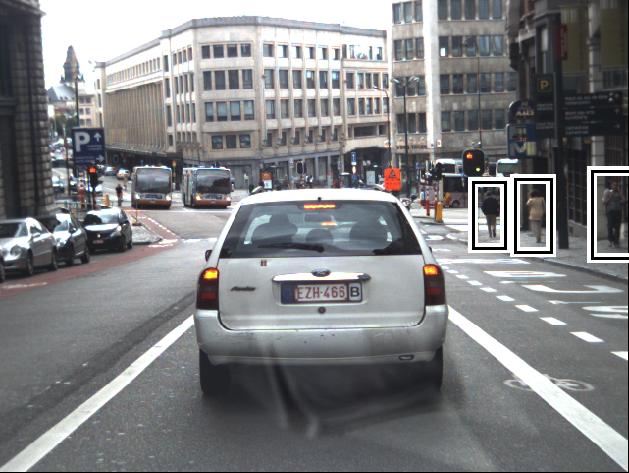
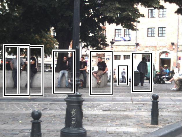
Figure 9: Top two rows: Pedestrian detection examples on TUD-Brussels data sets. Last row: False positive examples made by our detector. Most false positive examples usually contain patterns that mimic the contour of human shoulders or vertical gradients that mimic the torso and leg boundaries.

TABLE II: Examples of top $10$ retrieval results for bicycle (Graz data sets). Red bounding box indicates retrieval error

	C-BID
	AGH [10]
	LCH [49]
	LSI [53]
	SH [3]
	SphH [11]
	STH [48]

TABLE III: Examples of top $10$ retrieval results for sailing (Sports data sets). Red bounding box indicates retrieval error

	C-BID
	AGH [10]
	LCH [49]
	LSI [53]
	SH [3]
	SphH [11]
	STH [48]

V Conclusion

We have proposed a novel learning-based approach to building compact binary embeddings. The method is distinguished from other embedding techniques in that it exploits extra information in the form of a set of class labels and pair-wise proximity on the training data set. Although this learning-based approach is relatively computationally expensive, it needs only be carried out once offline. Exploiting previously ignored class-label information allows the method to generate embedded features which outperform their original high-dimensional counterparts. Experimental results demonstrate the effectiveness of our approach for both parametric and non-parametric models. Future works include applying the proposed formulation to multi-label classification, building hierarchical binary output codes and automatically generating the class labels for the training set.

Appendix A General convex loss with arbitrary regularization

In this appendix, we generalize our approach to arbitrary regularization. We first consider the logistic loss with $\ell_{\infty}$ penalty. The learning problem for the logistic loss in the $\ell_{\infty}$ regularization framework can be expressed as

$$\min_{{\boldsymbol{W}},{\boldsymbol{\rho}}}\; {\textstyle\sum}_{{\tau},r}\log\left(1+\exp(-\rho_{{\tau},r})\right)+\nu\|{\boldsymbol{W}}\|_{\infty}\quad$$ (17)

$$\mathop{\mathrm{s.t.\!\!:}}\nolimits\; \rho_{{\tau},r}={{\boldsymbol{a}}_{({\tau}|r)}}{\boldsymbol{w}}_{{y_{{\tau}}}}-{{\boldsymbol{a}}_{({\tau}|r)}}{\boldsymbol{w}}_{r},\forall{\tau},r;\;{\boldsymbol{W}}\geq 0.$$

Its Lagrange dual can be written as

$$\max_{{\boldsymbol{U}},{\boldsymbol{Q}}}\quad -{\textstyle\sum}_{{\tau},r}\Bigl{[}u_{{\tau},r}\log\left(u_{{\tau},r}\right)+$$ (18)

$$\left(1-u_{{\tau},r}\right)\log\left(1-u_{{\tau},r}\right)\Bigr{]}+\lambda\|{\boldsymbol{Q}}\|_{1}$$

$$\mathop{\mathrm{s.t.\!\!:}}\nolimits\quad {\textstyle\sum}_{{\tau}}\bigl{[}\delta_{r,{y_{{\tau}}}}\left(\textstyle\sum_{l}u_{{\tau},l}\right)-u_{{\tau},r}\bigr{]}{{\boldsymbol{a}}_{({\tau}|r)}}\leq\nu{\boldsymbol{q}}_{:r},\forall r;$$

${\boldsymbol{q}}_{:r}$ denotes the $r$-th column of ${\boldsymbol{Q}}$ and ${\boldsymbol{Q}}\geq 0$. Here the sub-problem for generating the most violated constraint is

$$h^{\ast}(\cdot)=\mathop{\mathrm{argmax}}\limits_{h(\cdot)\in\mathcal{H},r}\;{\textstyle\sum}_{{\tau}}(\delta_{r,{y_{{\tau}}}}\left(\textstyle\sum_{l}u_{{\tau},l}\right)-u_{{\tau},r}){a_{({\tau}|r)}}.$$ (19)

Although the subproblem for generating the binary function (weak learner) for both $\ell_{1}$ and $\ell_{\infty}$ penalties are the same, the solution to the primal variables, ${\boldsymbol{W}}$, are different. In our implementation, we solve the primal problem because the size of the primal problem is much smaller than the size of the dual problem.

Let us assume any general convex loss functions and arbitrary regularization penalties, the optimization problem can be rewritten as,

$$\min_{{\boldsymbol{W}},{\boldsymbol{\rho}}}\; {\textstyle\sum}_{{\tau},r}\Theta(\rho_{{\tau},r})+\nu\Omega({\boldsymbol{W}})$$ (20)

$$\;\mathop{\mathrm{s.t.\!\!:}}\nolimits\; \rho_{{\tau},r}={{\boldsymbol{a}}_{({\tau}|r)}}{\boldsymbol{w}}_{{y_{{\tau}}}}-{{\boldsymbol{a}}_{({\tau}|r)}}{\boldsymbol{w}}_{r},\forall{\tau},r;\ \text{and}\ {\boldsymbol{W}}\geq 0.$$

The Lagrangian of (20) is

$${\varLambda} ={\textstyle\sum}_{{\tau},r}\Theta\left(\rho_{{\tau},r}\right)+\nu\Omega({\boldsymbol{W}})$$ (21)

$$\;-{\textstyle\sum}_{{\tau},r}u_{{\tau},r}(\rho_{{\tau},r}-{{\boldsymbol{a}}_{({\tau}|r)}}{\boldsymbol{w}}_{{y_{{\tau}}}}+{{\boldsymbol{a}}_{({\tau}|r)}}{\boldsymbol{w}}_{r})-\operatorname{\bf Tr}({\boldsymbol{P}}^{\!\top}{\boldsymbol{W}}),$$

Following our derivation for the $\ell_{1}$ regularized logistic loss, the Lagrange dual can be written as,

$$\min_{{\boldsymbol{U}},{\boldsymbol{Q}}}\; {\textstyle\sum}_{{\tau},r}\Theta^{\ast}(-u_{{\tau},r})+\lambda\Omega^{\ast}({\boldsymbol{Q}})$$ (22)

$$\mathop{\mathrm{s.t.\!\!:}}\nolimits\; {\textstyle\sum}_{{\tau}}\bigl{[}\delta_{r,{y_{{\tau}}}}\left(\textstyle\sum_{l}u_{{\tau},l}\right)-u_{{\tau},r}\bigr{]}{{\boldsymbol{a}}_{({\tau}|r)}}\leq\nu{\boldsymbol{q}}_{:r},\forall r;$$

${\boldsymbol{Q}}\geq 0$. Here $\Theta^{\ast}(\cdot)$ is the Fenchel dual function of $\Theta(\cdot)$ and $\Omega^{\ast}(\cdot)$ is the Fenchel conjugate of $\Omega(\cdot)$.

References

- [1] A. Andoni and P. Indyk, “Near-optimal hashing algorithms for approximate nearest neighbor in high dimensions,” Communications of the ACM, vol. 51, no. 1, pp. 117 122, 2008.
- [2] Y. Liu, F. Wu, Y. Yang, Y. Zhuang, and A. G. Hauptmann, “Spline regression hashing for fast image search,” IEEE Trans. Image Proc., vol. 21, no. 10, pp. 4480–4491, 2012.
- [3] Y. Weiss, A. Torralba, and R. Fergus, “Spectral hashing,” in Proc. Adv. Neural Inf. Process. Syst., 2008.
- [4] A. Demiriz, K. P. Bennett, and J. Shawe-Taylor, “Linear programming boosting via column generation,” Mach. Learn., vol. 46, no. 1-3, pp. 225–254, 2002.
- [5] C. Shen, J. Kim, L. Wang, and A. van den Hengel, “Positive semidefinite metric learning using boosting-like algorithms,” J. Mach. Learn. Res., vol. 13, pp. 1007–1036, 2012.
- [6] M. Datar, N. Immorlica, P. Indyk, and V. Mirrokni, “Locality-sensitive hashing scheme based on p-stable distributions,” in Proc. of Symp. on Comp. Geometry, 2004.
- [7] Y. Ke, R. Sukthankar, and L. Huston, “Efficient near-duplicate detection and sub-image retrieval,” in Proc. of ACM Multimedia, 2004.
- [8] O. Chum, J. Philbin, M. Isard, and A. Zisserman, “Scalable near identical image and shot detection,” in Proc. of Int. Conf. on Image and Video Retrieval, 2007.
- [9] A. Frome and J. Malik, Object Recognition Using Locality-Sensitive Hashing of Shape Contexts, The MIT Press, 2005.
- [10] W. Liu, J. Wang, S. Kumar, and S.-F. Chang, “Hashing with graphs,” in Proc. Int. Conf. Mach. Learn., 2011.
- [11] J. Heo, Y. Lee, J. He, S. F. Chang, and S. E. Yoon, “Spherical hashing,” in Proc. IEEE Conf. Comp. Vis. Patt. Recogn., 2012.
- [12] S. Lazebnik, C. Schmid, and J. Ponce, “Beyond bags of features: Spatial pyramid matching for recognizing natural scene categories,” in Proc. IEEE Conf. Comp. Vis. Patt. Recogn., 2006.
- [13] L. Torresani, M. Szummer, and A. Fitzgibbon, “Efficient object category recognition using classemes,” in Proc. Eur. Conf. Comp. Vis., 2010.
- [14] L. J. Li, H. Su, L. Fei-Fei, and E. P. Xing, “Object bank: A high-level image representation for scene classification & semantic feature sparsification,” in Proc. Adv. Neural Inf. Process. Syst., 2010.
- [15] A. Bergamo, L. Torresani, and A. Fitzgibbon, “Picodes: Learning a compact code for novel-category recognition,” in Proc. Adv. Neural Inf. Process. Syst., 2011.
- [16] A. Bergamo and L. Torresani, “Meta-class features for large-scale object categorization on a budget,” in Proc. IEEE Conf. Comp. Vis. Patt. Recogn., 2012.
- [17] S. Bengio, J. Weston, and D. Grangier, “Label embedding trees for large multi-class tasks,” in Proc. Adv. Neural Inf. Process. Syst., 2010.
- [18] O. Boiman, E. Shechtman, and M. Irani, “In defense of nearest-neighbor based image classification,” in Proc. IEEE Conf. Comp. Vis. Patt. Recogn., 2008.
- [19] Y. L. Boureau, F. Bach, Y. LeCun, and J. Ponce, “Learning mid-level features for recognition,” in Proc. IEEE Conf. Comp. Vis. Patt. Recogn., 2010.
- [20] J. Yang, K. Yu, Y. Gong, and T. S. Huang., “Linear spatial pyramid matching using sparse coding for image classification,” in Proc. IEEE Conf. Comp. Vis. Patt. Recogn., 2009.
- [21] J. Wang, J. Yang, K. Yu, F. Lv, T. Huang, and Y. Gong, “Locality-constrained linear coding for image classification,” in Proc. IEEE Conf. Comp. Vis. Patt. Recogn., 2010.
- [22] Z. Wang, J. Feng, S. Yan, and H. Xi, “Linear distance coding for image classification,” IEEE Trans. Image Proc., vol. 22, no. 2, pp. 537–548, 2013.
- [23] R. Behmo, P. Marcombes, A. Dalalyan, and V. Prinet, “Towards optimal naive bayes nearest neighbor,” in Proc. Eur. Conf. Comp. Vis., 2010.
- [24] T Tuytelaars, M. Fritz, K. Saenko, and T. Darrell, “The NBNN kernel,” in Proc. IEEE Int. Conf. Comp. Vis., 2011.
- [25] S. McCann and D. G. Lowe, “Local naive bayes nearest neighbor for image classification,” in Proc. IEEE Conf. Comp. Vis. Patt. Recogn., 2012.
- [26] Z. Wang, Y. Hu, and L.-T. Chia, “Image-to-Class distance metric learning for image classification,” in Proc. Eur. Conf. Comp. Vis., 2010.
- [27] David G. Lowe, “Distinctive image features from scale-invariant keypoints,” Int. J. Comp. Vis., vol. 60, no. 2, pp. 91–110, 2004.
- [28] S. Zhang, Q. Tian, K. Lu, Q. Huang, and W. Gao, “Edge-SIFT: Discriminative binary descriptor for scalable partial-duplicate mobile search,” IEEE Trans. Image Proc., vol. 22, no. 7, pp. 2889–2902, 2013.
- [29] H. Bay, T. Tuytelaars, and L. Van Gool, “SURF: Speeded up robust features,” in Proc. Eur. Conf. Comp. Vis., 2006.
- [30] K. Kira and L. A. Rendell, “A practical approach to feature selection,” in Proc. Int. Conf. Mach. Learn., 1992.
- [31] Y. Sun, S. Todorovic, and S. Goodison, “Local-learning-based feature selection for high-dimensional data analysis,” IEEE Trans. Pattern Anal. Mach. Intell., vol. 32, no. 9, pp. 1610–1626, 2010.
- [32] K. Q. Weinberger, J. Blitzer, and L. K. Saul, “Distance metric learning for large margin nearest neighbor classification,” in Proc. Adv. Neural Inf. Process. Syst., 2006.
- [33] L. J. P. van der Maaten and K. Q. Weinberger, “Stochastic triplet embedding,” in IEEE Intl. Workshop on Mach. Learn. for Sig. Proc., 2012.
- [34] X. Liu and T. Yu, “Gradient feature selection for online boosting,” in Proc. IEEE Int. Conf. Comp. Vis., 2007.
- [35] C. Zhu, R. H. Byrd, P. Lu, and J. Nocedal, “Algorithm 778: L-bfgs-b: Fortran subroutines for large-scale bound-constrained optimization,” ACM Trans. Math. Software, vol. 23, no. 4, pp. 550–560, 1997.
- [36] Q.V. Le, J. Ngiam, A. Coates, A. Lahiri, B. Prochnow, and A.Y. Ng., “On optimization methods for deep learning.,” in Proc. Int. Conf. Mach. Learn., 2011.
- [37] M. Norouzi, D. Fleet, and R. Salakhutdinov, “Hamming distance metric learning,” in Proc. Adv. Neural Inf. Process. Syst., 2012.
- [38] A. Vedaldi and A. Zisserman, “Efficient additive kernels via explicit feature maps,” in Proc. IEEE Conf. Comp. Vis. Patt. Recogn., 2010.
- [39] A. Vedaldi and B. Fulkerson, “VLFeat: An open and portable library of computer vision algorithms,” http://www.vlfeat.org/, 2008.
- [40] M. Aly, M. Munich, and P. Perona, “Indexing in large scale image collections: Scaling properties and benchmark,” in IEEE Workshop on Apps. of Comp. Vis., 2011.
- [41] P. Viola and M. J. Jones, “Robust real-time face detection,” Int. J. Comp. Vis., vol. 57, no. 2, pp. 137–154, 2004.
- [42] S. Munder and D. M. Gavrila, “An experimental study on pedestrian classification,” IEEE Trans. Pattern Anal. Mach. Intell., vol. 28, no. 11, pp. 1863–1868, 2006.
- [43] N. Dalal and B. Triggs, “Histograms of oriented gradients for human detection,” in Proc. IEEE Conf. Comp. Vis. Patt. Recogn., 2005.
- [44] C. Wojek, S. Walk, and B. Schiele, “Multi-cue onboard pedestrian detection,” in Proc. IEEE Conf. Comp. Vis. Patt. Recogn., 2009.
- [45] P. Dollár, C. Wojek, B. Schiele, and P. Perona, “Pedestrian detection: An evaluation of the state of the art,” IEEE Trans. Pattern Anal. Mach. Intell., vol. 34, no. 4, pp. 743–761, 2012.
- [46] A. Torralba, K. P. Murphy, W. T. Freeman, and M. A. Rubin, “Context-based vision system for place and object recognition,” in Proc. IEEE Int. Conf. Comp. Vis., 2003.
- [47] L. Bo, K. Lai, X. Ren, and D. Fox, “Object recognition with hierarchical kernel descriptors,” in Proc. IEEE Conf. Comp. Vis. Patt. Recogn., 2011.
- [48] D. Zhang, J. Wang, D. Cai, and J. Lu, “Self-taught hashing for fast similarity search,” in ACM SIGIR, 2010.
- [49] D. Zhang, J. Wang, D. Cai, and J. Lu., “Laplacian co-hashing of terms and documents,” in European Conf. on IR Res., 2010.
- [50] J. Wu and J. M. Rehg, “CENTRIST: A visual descriptor for scene categorization,” IEEE Trans. Pattern Anal. Mach. Intell., vol. 33, no. 8, pp. 1489–1501, 2011.
- [51] R.-E. Fan, K.-W. Chang, C.-J. Hsieh, X.-R. Wang, and C.-J. Lin, “LIBLINEAR: A library for large linear classification,” J. Mach. Learn. Res., vol. 9, pp. 1871–1874, 2008.
- [52] Y. Weiss, R. Fergus, and A. Torralba, “Multidimensional spectral hashing,” in Proc. Eur. Conf. Comp. Vis., 2012.
- [53] S. C. Deerwester, S. T. Dumais, T. K. Landauer, G. W. Furnas, and R. A. Harshman, “Indexing by latent semantic analysis,” Journal American Socity for Information Science, vol. 41, no. 6, pp. 391–407, 1990.