C/O abundance ratios, iron depletions, and infrared dust features in Galactic Planetary Nebulae

Abstract

We study the dust present in 56 Galactic planetary nebulae (PNe) through their iron depletion factors, their C/O abundance ratios (in 51 objects), and the dust features that appear in their infrared spectra (for 33 objects). Our sample objects have deep optical spectra of good quality, and most of them also have ultraviolet observations. We use these observations to derive the iron abundances and the C/O abundance ratios in a homogeneous way for all the objects. We compile detections of infrared dust features from the literature and we analyze the available Spitzer/IRS spectra. Most of the PNe have C/O ratios below one and show crystalline silicates in their infrared spectra. The PNe with silicates have C/O $<1$, with the exception of Cn 1-5. Most of the PNe with dust features related to C-rich environments (SiC or the 30 $\mu$m feature usually associated to MgS) have C/O $\gtrsim 0.8$. PAHs are detected over the full range of C/O values, including 6 objects that also show silicates. Iron abundances are low in all the objects, implying that more than 90% of their iron atoms are deposited into dust grains. The range of iron depletions in the sample covers about two orders of magnitude, and we find that the highest depletion factors are found in C-rich objects with SiC or the 30 $\mu$m feature in their infrared spectra, whereas some of the O-rich objects with silicates show the lowest depletion factors.

1. Introduction

Planetary nebulae (PNe) are suitable sites to study the evolution of dust grains since their progenitors, asymptotic giant branch (AGB) stars, are among the most efficient sources of circumstellar dust in the Galaxy (Whittet, 2003). These stars lose large amounts of material and create circumstellar envelopes with both low temperatures (below 1500 K in the regions of dust formation) and high densities ($\sim$ 10¹³ cm^-3), where dust grains are efficiently formed.

In Delgado-Inglada et al. (2009), we studied iron depletions into dust grains in a sample of 33 Galactic disk PNe. Iron is an important contributor to the mass of dust grains (Sofia et al., 1994), and its gaseous abundance can be used as a proxy for the amount of depletion of other elements. We found low iron gaseous abundances in all the objects, suggesting that more than 90% of their iron atoms are located in grains. We also found that the range of iron depletions covers about two orders of magnitude, which may be a consequence of differences in the formation and evolution of the grains in the different nebulae. We did not find any obvious correlation between iron abundances and parameters related to the nebular age (such as the nebular radius or the surface brightness) or to the dominant chemistry in the nebulae (C-rich or O-rich) that could provide clues on the reasons behind the different depletions. However, the information available for the studied sample was scarce.

On the other hand, the dust features that appear in the infrared spectra of PNe provide information on the composition of their dust grains. In our galaxy, PNe with crystalline silicates, many of them also with PAHs, are the most numerous (Gutenkunst et al., 2008; Perea-Calderón et al., 2009; Stanghellini et al., 2012). Besides, a general correlation has been found between infrared features and C/O abundance ratios: Magellanic Clouds PNe with silicates have C/O $<1$, and those with carbonaceous dust have C/O $>1$, although for Galactic PNe the situation is less clear (Casassus et al., 2001a; Cohen & Barlow, 2005; Stanghellini et al., 2007; Waters et al., 1998).

The relative abundances of carbon and oxygen in the envelope of an AGB star depends on the nucleosynthesis processes occurring in the inner regions, which in turn depends on the mass of the progenitor star and on its initial metallicity. In our galaxy, we expect stars to be born with an almost solar C/O ratio (C/O $\sim 0.5$, Allende Prieto et al. 2002), that may change during the evolution of the star depending on its initial mass. Theoretical models (see, e.g., Marigo et al., 2003; Karakas et al., 2009) predict that the less massive progenitors (M_∗ $\lesssim 1.5$–2 M_⊙) will remain O-rich during their whole evolution. Stars with masses in the range $\sim$ 2–4 M_⊙ may evolve from O-rich to C-rich due to the third dredge-up process that enriches the surface of the AGB star with carbon. In the most massive progenitors (M_∗ $\gtrsim$ 4–5 M_⊙), the hot bottom burning process occurs efficiently and, since it converts carbon into nitrogen via the CN cycle, it can prevent the formation of a C-rich star.

The value of C/O in a dust-forming stellar envelope defines whether the dust particles will be C-rich or O-rich. If carbon is more abundant than oxygen, all the oxygen atoms will be trapped in CO molecules and carbon atoms will be available to form C-rich compounds, such as graphite, amorphous carbon, or silicon carbide (SiC). If oxygen is more abundant than carbon, all the carbon atoms will be trapped by CO and the remaining oxygen atoms will form O-rich grains like silicates and oxides.

Oxygen rich nebulae could have iron deposited in metallic iron grains, silicates and oxides, whereas C-rich nebulae are expected to have their iron atoms in the form of metallic grains, Fe₃C, FeSi, FeS, and FeS₂ (Whittet, 2003). Therefore, iron depletion factors could be different in C-rich and O-rich PNe. The C-rich or O-rich chemistry may be studied from the C/O abundance ratios or from the infrared dust features, and we expect both to be related. In principle, C-rich features such as SiC are expected in PNe with C/O $>1$ (but see Bond et al., 2010) whereas O-rich features like silicates are expected in PNe with C/O $<1$. ISO and Spitzer telescopes allow us to detect and identify several dust species in the spectra of PNe and therefore, to classify PNe as C-rich or O-rich according to the observed features.

Here, we extend the work performed in Delgado-Inglada et al. (2009) by studying a sample of Galactic PNe that nearly doubles the previous one and also by analyzing possible correlations between their iron depletions, C/O abundance ratios, and infrared dust features.

The paper is organized as follows. In Section 2 we describe our sample of Galactic PNe, whereas in Section 3 we present the calculation of electron temperatures and densities for all the objects. Section 4 contains an extensive discussion of the iron abundance and depletion factor calculations. Section 5 details the calculation of C/O abundance ratios from collisionally excited lines (CELs) and recombination lines (RLs), and the comparison between these two estimates. The compilation of infrared dust features observed in the sample is presented in Section 6. In Section 7 we discuss our results and study the correlation between iron abundances, C/O values, and dust features in our sample of PNe. Our conclusions are presented in Section 8.

2. The Sample

Our sample consists of 56 Galactic PNe with published spectra of relatively high spectral resolution and deep enough to detect the lines we need to calculate physical conditions and iron abundances. The sample includes 28 Galactic PNe studied in Delgado-Inglada et al. (2009), but we exclude nebulae with electron densities above 25 000 $\rm{cm}^{-3}$ since it is difficult to derive reliable physical conditions and chemical abundances in these objects (Delgado-Inglada et al., 2009). Besides, we set an upper limit on the $I(\mbox{{He~{}II}~{}}\lambda 4686)/I(\mbox{H}\beta)$ intensity ratio of 0.6, in order to avoid high excitation PNe for which the iron correction scheme adopted here may not apply (Rodríguez & Rubin, 2005). The final sample of 56 PNe is presented in Table 2.

Table 1Physical conditions

Object	$n_{\rm e}$ ($\rm{cm}^{-3}$)	$T_{\rm e}$[N II] (K)	$T_{\rm e}$[O III] (K)	Ref.
Cn 1-5 (catalog )	$4200^{+1800}_{-1200}$	$7300\pm 200$	$8800\pm 100$	1
Cn 3-1 (catalog )	$7200^{+1800}_{-1200}$	$7800\pm 200$	$7800\pm 400$	2
DdDm 1 (catalog )	$5300^{+3400}_{-1800}$	$13100^{+600}_{-800}$	$12300\pm 300$	2
H 1-41 (catalog )	$1600^{+900}_{-500}$	$9800^{+800}_{-900}$	$9800\pm 200$	1
H 1-42 (catalog )	$8700^{+2600}_{-1700}$	$11500\pm 1200$	$10200\pm 200$	1
H 1-50 (catalog )	$11200^{+2300}_{-1600}$	$11000^{+400}_{-500}$	$11000\pm 200$	1
Hu 1-1 (catalog )	$1800\pm 300$	$11500^{+400}_{-300}$	$12000\pm 300$	2
Hu 2-1 (catalog )	$9000^{+7500}_{-2900}$	$12300^{+700}_{-1300}$	$11000^{+200}_{-300}$	2
IC 418 (catalog )	$10300^{+1700}_{-1400}$	$9400\pm 300$	$8900\pm 200$	3
IC 1747 (catalog )	$3800^{+800}_{-600}$	$12400^{+400}_{-500}$	$10500\pm 200$	2
IC 2165 (catalog )	$4500^{+600}_{-500}$	$13100\pm 500$	$14600\pm 400$	4
IC 3568 (catalog )	$2100^{+700}_{-500}$	$18800^{+1200}_{-2900}$	$11500\pm 300$	5
IC 4191 (catalog )	$14800^{+2400}_{-2300}$	$11300\pm 500$	$10300\pm 200$	6
IC 4406 (catalog )	$2400^{+400}_{-300}$	$10200\pm 300$	$10000\pm 200$	6
IC 4593 (catalog )	$1700^{+700}_{-500}$	$9800^{+900}_{-1000}$	$8500^{+200}_{-300}$	7
IC 4699 (catalog )	$2500^{+1700}_{-900}$	$19500^{+500}_{-4600}$	$11800\pm 300$	1
IC 4846 (catalog )	$10100^{+4000}_{-2400}$	$12100^{+2000}_{-2100}$	$10600\pm 400$	8
IC 5217 (catalog )	$5100^{+1300}_{-1000}$	$13700^{+3400}_{-2800}$	$10800\pm 400$	9
JnEr 1 (catalog )	$400^{+600}_{-300}$	$10300^{+900}_{-800}$	$12700^{+2000}_{-1000}$	7
M 1-20 (catalog )	$12100^{+4900}_{-3200}$	$11000^{+600}_{-700}$	$9900\pm 200$	1
M 1-42 (catalog )	$1400^{+300}_{-200}$	$9100\pm 200$	$10000\pm 200$	10
M 1-73 (catalog )	$4300^{+1600}_{-900}$	$8800^{+200}_{-300}$	$7300\pm 100$	2
M 2-4 (catalog )	$8700^{+3100}_{-2200}$	$10000^{+400}_{-500}$	$8600\pm 100$	1
M 2-6 (catalog )	$10300^{+6200}_{-3500}$	$10600^{+600}_{-800}$	$10100\pm 200$	1
M 2-27 (catalog )	$13600^{+3500}_{-2300}$	$8800^{+300}_{-400}$	$8300\pm 100$	1
M 2-31 (catalog )	$7700^{+2300}_{-1500}$	$11400^{+400}_{-500}$	$9900\pm 200$	1
M 2-33 (catalog )	$3100^{+3600}_{-1600}$	$9200^{+1000}_{-1300}$	$8000\pm 100$	1
M 2-36 (catalog )	$4700^{+700}_{-600}$	$9200^{+400}_{-100}$	$8400\pm 100$	10
M 2-42 (catalog )	$4800^{+2400}_{-1600}$	$10200^{+400}_{-500}$	$8500\pm 100$	1
M 3-7 (catalog )	$4700^{+2400}_{-1500}$	$8600\pm 300$	$7700\pm 100$	1
M 3-29 (catalog )	$800^{+400}_{-200}$	$9000^{+600}_{-700}$	$9200\pm 200$	1
M 3-32 (catalog )	$2900^{+800}_{-600}$	$17400\pm 2500$	$8900\pm 200$	1
MyCn 18 (catalog )	$9400^{+1700}_{-1300}$	$9800\pm 300$	$7400\pm 100$	6
NGC 40 (catalog )	$1300\pm 200$	$8600\pm 200$	$10600\pm 200$	5
NGC 2392 (catalog )	$2200^{+1900}_{-1000}$	$12700^{+1600}_{-1300}$	$14600^{+900}_{-1000}$	7
NGC 3132 (catalog )	$700\pm 200$	$9700^{+200}_{-300}$	$9600\pm 200$	6
NGC 3242 (catalog )	$2400\pm 400$	$12400\pm 400$	$11900\pm 300$	6
NGC 3587 (catalog )	$2400^{+1900}_{-1300}$	$10900\pm 1000$	$11600\pm 500$	7
NGC 3918 (catalog )	$7100^{+1100}_{-900}$	$10800^{+300}_{-400}$	$12700\pm 300$	6
NGC 5882 (catalog )	$5100^{+700}_{-500}$	$10600\pm 300$	$9400\pm 200$	6
NGC 6153 (catalog )	$3900^{+500}_{-400}$	$10500\pm 300$	$9200\pm 200$	11
NGC 6210 (catalog )	$5800^{+4500}_{-2100}$	$11000^{+400}_{-300}$	$9600\pm 200$	5
NGC 6439 (catalog )	$6000^{+800}_{-700}$	$9700\pm 300$	$10400\pm 200$	1
NGC 6543 (catalog )	$5800^{+2000}_{-1400}$	$10000^{+500}_{-600}$	$7900\pm 200$	12
NGC 6565 (catalog )	$1600\pm 300$	$10600\pm 300$	$10400\pm 200$	1
NGC 6572 (catalog )	$17900^{+4300}_{-2700}$	$12000^{+600}_{-700}$	$10400\pm 200$	5
NGC 6620 (catalog )	$2900\pm 400$	$9000\pm 200$	$9600\pm 200$	1
NGC 6720 (catalog )	$700\pm 200$	$10600\pm 300$	$10700^{+300}_{-200}$	5
NGC 6741 (catalog )	$6700\pm 800$	$10800^{+400}_{-300}$	$12600\pm 300$	5
NGC 6803 (catalog )	$9300^{+1200}_{-900}$	$10700\pm 300$	$9700\pm 200$	2
NGC 6818 (catalog )	$2300\pm 300$	$11400\pm 400$	$13400^{+400}_{-300}$	6
NGC 6826 (catalog )	$2100\pm 300$	$10600\pm 500$	$9400\pm 200$	5
NGC 6884 (catalog )	$8900^{+1300}_{-1000}$	$11600\pm 400$	$11100\pm 300$	5
NGC 7026 (catalog )	$7500^{+1100}_{-800}$	$9700\pm 300$	$9300\pm 200$	2
NGC 7662 (catalog )	$3000\pm 400$	$13000^{+500}_{-400}$	$13400\pm 400$	5
Vy 2-1 (catalog )	$5400^{+2600}_{-1800}$	$9300^{+100}_{-700}$	$7900\pm 100$	1

References. — Line intensities from: (1) Wang & Liu (2007), (2) Wesson et al. (2005), (3) Sharpee et al. (2003), (4) Hyung (1994), (5) Liu et al. (2004b), (6) Tsamis et al. (2003), (7) Delgado-Inglada et al. (2009), (8) Hyung et al. (2001b), (9) Hyung et al. (2001a), (10) Liu et al. (2001), (11) Liu et al. (2000), (12) Wesson & Liu (2004).

3. Physical conditions

We derive electron densities and temperatures, $n_{\rm e}$ and $T_{\rm e}$, using the routine temden from the package nebular (Shaw, 1995) in IRAF. For each object, we calculate two temperatures from the observed intensity ratios [N II] $\lambda 5755/(\lambda 6548+\lambda 6584)$ and [O III] $\lambda 4363/(\lambda 4959+\lambda 5007)$ to characterize the low- and high-ionization regions, respectively. We also derive an average density from the available diagnostic ratios among the following: [O II] $\lambda 3726/\lambda 3729$, [S II] $\lambda 6716/\lambda 6731$, [Cl III] $\lambda 5518/\lambda 5538$, and [Ar IV] $\lambda 4711/\lambda 4740$. We use the default atomic data in IRAF except for Cl⁺⁺ and O⁺: for these ions we find densities in better agreement with those obtained from the other diagnostic ratios using the collision strengths of Krueger & Czyzak (1970) and Tayal (2007) and the transition probabilities of Mendoza & Zeippen (1982) and Zeippen (1982).

Rubin (1986) found that a significant fraction of the intensity of the [N II] $\lambda$5755 line can arise from recombinations of N⁺⁺. If this effect is not taken into account, the value of $T_{\rm e}$[N II] can be overestimated in those objects where N⁺⁺ is an important contributor to the total abundance of nitrogen. The contribution of recombination to [N II] $\lambda$5755 can be estimated using the expression derived by Liu et al. (2000), which depends on the N⁺⁺ abundance. This ionic abundance can be obtained either from infrared/ultraviolet collisionally excited lines or from optical recombination lines, leading in each case to different results. Thus, the correction is somewhat uncertain and we do not apply it here. However, we estimate an upper limit of the effect it could have on our results by using the highest possible values for the N⁺⁺ abundances, which are those implied by recombination lines. We find that in many of our objects $T_{\rm e}$[N II] would change by less than 10%. The objects with the largest differences in $T_{\rm e}$[N II] are DdDm 1, IC 3568, IC 4699, M 3-32, and NGC 3242, where they reach 30–50%. For these objects, this implies values of Fe/O up to 0.4 dex lower or up to 0.2 dex higher, depending on which ionization correction approach we use (see § 4.2). Hence, the iron abundances derived for these 5 PNe have this additional amount of uncertainty.

We calculate the uncertainties of the physical conditions and the ionic and total abundances of O and Fe using Montecarlo simulations, which assume that the errors in the line intensities follow Gaussian distributions. The line intensity errors are those given in the references listed in Table 2. Each Montecarlo run samples the Gaussian distributions of all the lines in order to provide new values for $T_{\rm e}$, $n_{\rm e}$, and all the ionic and total abundances described in § 4.1 and § 4.2 below. The errors listed for the calculated quantities define a confidence interval of 68$\%$ (equivalent to one standard deviation in a Gaussian distribution).

Table 2 presents the physical conditions and their associated uncertainties for our sample PNe. The values are similar to the ones obtained in Delgado-Inglada et al. (2009) for the objects in common. The highest differences are for the values of $n_{\rm e}$, and there are two reasons for that. First, we use here one more diagnostic ratio for the density, [O II] $\lambda 3726/\lambda 3729$. Second, whereas Delgado-Inglada et al. (2009) derive the final $n_{\rm e}$ as the weighted mean of the values implied by the available diagnostic ratios, here the final $n_{\rm e}$ is the median value of the density distribution obtained from averaging the $n_{\rm e}$ values calculated in each run of the Montecarlo simulation. One of the objects with significant differences is NGC 3587, where Delgado-Inglada et al. (2009) used the [S II] density diagnostic and found $n_{\rm e}$ $<100$ $\rm{cm}^{-3}$, whereas here we also use the [O II] diagnostic and find $n_{\rm e}$$=2400$ $\rm{cm}^{-3}$. This change in $n_{\rm e}$ implies a change in $T_{\rm e}$[N II] from 9800 K to 10900 K. In general, $T_{\rm e}$ differences are smaller, around 100 K in most of the objects. The new values derived for the physical conditions imply oxygen abundances that are within $\pm$0.15 dex of the old values. These differences illustrate the abundance uncertainties introduced by the approach chosen to perform the calculations.

4. Iron depletion factors

4.1. Ionic abundances

The total iron abundances of the sample PNe are calculated from the Fe⁺⁺ abundance (and Fe⁺ in some cases) along with ionization correction factors (ICFs) based on the ionic and total oxygen abundances. On the other hand, the ICF we use for oxygen is based on the He⁺ and He⁺⁺ abundances. Hence, we derive all these ionic abundances using the densities and temperatures from Table 2, in particular $T_{\rm e}$[N II] for O⁺, Fe⁺, and Fe⁺⁺, and $T_{\rm e}$[O III] for O⁺⁺, He⁺, and He⁺⁺.

The values of O⁺/H⁺ and O⁺⁺/H⁺ are calculated using the intensities of the [O II] $\lambda\lambda 3726+29$ and [O III] $\lambda\lambda 4959,5007$ lines with respect to H$\beta$ and the routine ionic of the package nebular in IRAF with the changes in atomic data mentioned in § 3.

The values of He⁺/H⁺ are based on He I $\lambda$6678 and the calculations of Benjamin et al. (1999). In DdDm 1 and IC 2165 we replace our computed He⁺ abundances (He⁺/H${}^{+}=0.041$ and 0.042) with the average of the He⁺ abundances derived from the He I $\lambda$$\lambda$4471, 5876 lines by Hyung (1994) and Wesson et al. (2005), respectively. These authors suggest that the low values implied by the $\lambda$6678 line could be due to underlying absorption.

The values of He⁺⁺/H⁺ are derived using He II $\lambda$4686 and the emissivities of Storey & Hummer (1995). The H I emissivities are also from Storey & Hummer (1995).

We estimate the Fe⁺ abundances for eleven PNe using the emissivities of Bautista & Pradhan (1996) and [Fe II] $\lambda 8616$, one of the few [Fe II] lines which are not affected by fluorescence (Verner et al., 2000). In some cases where this line is not available we use instead [Fe II] $\lambda 7155$ and $I(\lambda 8616)/I(\lambda 7155)\sim 1$, as found by Rodríguez (1996) in several H II regions. The values of Fe⁺/Fe⁺⁺ for these eleven PNe go from 0.06 (M 3-7) to 0.80 (NGC 6565 and NGC 6741). Only five of the sample PNe would require a value for the Fe⁺ abundance in the ionization correction scheme described below, in § 4.2. The two of them where it is available show that its contribution is not likely to be critical, since it only increases the value of Fe/H by 0.08 dex (in NGC 40) and 0.17 dex (in IC 418). Some of the calculated values of Fe⁺/H⁺ are also used in the calculations described in § 4.3.

The Fe⁺⁺ ionic abundances are derived by solving the equations of statistical equilibrium (Osterbrock & Ferland, 2006) for a 34-level model atom, using the collision strengths of Zhang (1996) and the transition probabilities of Quinet (1996). We used PyNeb (Luridiana et al., 2012) to compare the results obtained with these atomic data with those implied by the recent calculations of Bautista et al. (2010). In the three nebulae with the largest numbers of [Fe III] lines (Cn 1-5, M 2-4, and M 2-6), we find differences lower than 5% in the final Fe⁺⁺ abundances, but the older atomic data lead to a better agreement in the Fe⁺⁺ abundances derived from all the available [Fe III] lines, with standard deviations of 32%/39% for the old/new atomic data (Cn 1-5), 12%/25%(M 2-4), and 23%/25% (M 2-6). We performed a similar comparison using 14 out of the 15 [Fe III] lines measured by Esteban et al. (2004) in the Orion Nebula (we excluded the line at 4926 Å because it leads to much higher abundances with both sets of atomic data). We find that the new atomic data lead to a Fe⁺⁺ abundance that is 15% lower, whereas the standard deviation changes from 15% to 30%. Hence, we perform our calculations using the older set of atomic data.

We use up to 9 [Fe III] lines for each object, excluding those suspected to be contaminated with nearby recombination lines. For the eight PNe in the sample with no [Fe III] lines in their spectra, we estimate upper limits to their Fe⁺⁺ abundances using the intensities reported for C IV $\lambda$4658 or O II $\lambda$4661. These lines are close in wavelength to [Fe III] $\lambda$4658, the brightest [Fe III] line for the physical conditions of our PNe. We use C IV $\lambda$4658 for IC 4406, IC 1747, JnEr 1, M 1-42, M 3-29, and NGC 7026, and O II $\lambda$4661 for H 1-41 and M 3-32. Some PNe show lines from higher iron ionization states; this will be discussed in § 4.3.

Table 2 presents all the computed ionic abundances and their uncertainties. The last column shows the number of [Fe III] lines used to derive the Fe⁺⁺ abundance in each object. The PNe where only upper limits are available are distinguished either with “1?”, when the C IV $\lambda$4658 line was used (note that this line could be a misidentification of [Fe III] $\lambda$4658), or with “–” when O II $\lambda$4661 was used.

Table 2Ionic Abundances: {X⁺ⁱ} = 12 + $\log$ (X⁺ⁱ/H⁺)

PN	{He+}	{He++}	{O+}	{O++}	{Fe+}	{Fe++}	Number of
	$\lambda$6678	$\lambda$4686	$\lambda\lambda$3726,3729	$\lambda\lambda$4959.5007	$\lambda$8616	average	[Fe III] lines
Cn 1-5	$11.08\pm 0.02$	–	$8.36\pm 0.11$	$8.68\pm 0.04$	5.23	$6.29^{+0.05}_{-0.07}$	8
Cn 3-1	$10.67\pm 0.02$	$7.52^{+0.11}_{-0.15}$	$8.68^{+0.12}_{-0.09}$	$7.26^{+0.11}_{-0.08}$	–	$5.57^{+0.06}_{-0.05}$	3
DdDm 1	$10.95\pm 0.02$	–	$7.38^{+0.31}_{-0.14}$	$7.91^{+0.05}_{-0.04}$	–	$5.76^{+0.08}_{-0.04}$	4
H 1-41	$10.96\pm 0.02$	$10.35\pm 0.02$	$7.27^{+0.19}_{-0.14}$	$8.50\pm 0.04$	–	$<4.85$	–
H 1-42	$11.05\pm 0.02$	$8.83\pm 0.02$	$7.10^{+0.23}_{-0.18}$	$8.54\pm 0.04$	4.50	$4.67^{+0.17}_{-0.14}$	3
H 1-50	$10.99\pm 0.02$	$10.04\pm 0.02$	$7.50^{+0.12}_{-0.10}$	$8.62\pm 0.04$	–	$4.54^{+0.10}_{-0.11}$	1
Hu 1-1	$10.93\pm 0.02$	$10.18\pm 0.02$	$8.00^{+0.06}_{-0.05}$	$8.40\pm 0.04$	–	$4.25^{+0.16}_{-0.22}$	1
Hu 2-1	$10.83\pm 0.02$	$8.39^{+0.03}_{-0.01}$	$7.44^{+0.34}_{-0.07}$	$8.19^{+0.05}_{-0.04}$	–	$4.88^{+0.05}_{-0.08}$	4
IC 418	$10.97\pm 0.02$	–	$8.34^{+0.07}_{-0.12}$	$8.06\pm 0.04$	3.89	$4.20^{+0.06}_{-0.05}$	5
IC 1747	$11.01\pm 0.02$	$10.04\pm 0.02$	$7.07^{+0.09}_{-0.06}$	$8.56\pm 0.04$	–	$<4.34$	1?
IC 2165	$10.74\pm 0.02$	$10.73\pm 0.02$	$6.80\pm 0.06$	$8.10\pm 0.04$	3.64	$4.58^{+0.06}_{-0.07}$	3
IC 3568	$10.96\pm 0.02$	$9.02\pm 0.02$	$5.69^{+0.24}_{-0.06}$	$8.36\pm 0.05$	–	$3.90^{+0.17}_{-0.10}$	2
IC 4191	$11.04\pm 0.02$	$10.08\pm 0.02$	$7.51^{+0.12}_{-0.11}$	$8.64\pm 0.04$	–	$4.38^{+0.10}_{-0.11}$	1
IC 4406	$10.97\pm 0.02$	$10.08\pm 0.02$	$8.28\pm 0.06$	$8.58\pm 0.04$	–	$<4.58$	1?
IC 4593	$11.00\pm 0.02$	$8.53^{+0.05}_{-0.06}$	$7.39^{+0.24}_{-0.16}$	$8.54\pm 0.06$	–	$5.39^{+0.16}_{-0.13}$	4
IC 4699	$10.92\pm 0.02$	$10.26\pm 0.02$	$6.14^{+0.36}_{-0.03}$	$8.40\pm 0.04$	–	$3.90^{+0.27}_{-0.13}$	1
IC 4846	$10.96\pm 0.02$	$8.68^{+0.11}_{-0.15}$	$7.03^{+0.40}_{-0.26}$	$8.48\pm 0.06$	–	$4.54^{+0.26}_{-0.19}$	2
IC 5217	$10.84^{+0.08}_{-0.10}$	$9.95\pm 0.04$	$6.59^{+0.41}_{-0.28}$	$8.63\pm 0.07$	–	$4.61^{+0.27}_{-0.30}$	1
JnEr 1	$11.29^{+0.08}_{-0.09}$	$10.25\pm 0.04$	$8.40^{+0.19}_{-0.18}$	$7.83^{+0.16}_{-0.13}$	–	$<5.49$	1?
M 1-20	$10.99\pm 0.02$	$7.61^{+0.12}_{-0.16}$	$7.46^{+0.21}_{-0.17}$	$8.53\pm 0.04$	–	$4.39^{+0.16}_{-0.17}$	1
M 1-42	$11.22\pm 0.02$	$10.04\pm 0.02$	$7.61^{+0.16}_{-0.05}$	$8.36^{+0.05}_{-0.04}$	–	$<5.53$	1?
M 1-73	$11.02\pm 0.02$	$8.99\pm 0.02$	$8.13^{+0.13}_{-0.09}$	$8.52\pm 0.05$	–	$5.42^{+0.07}_{-0.06}$	2
M 2-4	$11.08\pm 0.02$	–	$7.82^{+0.18}_{-0.13}$	$8.66\pm 0.04$	–	$5.49\pm 0.07$	9
M 2-6	$11.05\pm 0.02$	$8.93\pm 0.02$	$7.70^{+0.26}_{-0.18}$	$8.36\pm 0.04$	–	$5.34^{+0.11}_{-0.08}$	8
M 2-27	$11.13\pm 0.02$	$8.84\pm 0.02$	$7.83^{+0.16}_{-0.12}$	$8.82\pm 0.04$	–	$5.51^{+0.09}_{-0.06}$	2
M 2-31	$11.10\pm 0.02$	–	$7.30^{+0.13}_{-0.09}$	$8.62\pm 0.04$	–	$5.55^{+0.14}_{-0.15}$	1
M 2-33	$11.01\pm 0.02$	$8.92\pm 0.02$	$7.34^{+0.41}_{-0.19}$	$8.67\pm 0.04$	–	$5.30^{+0.24}_{-0.16}$	5
M 2-36	$11.01\pm 0.02$	$9.01\pm 0.02$	$7.64^{+0.10}_{-0.07}$	$8.71\pm 0.04$	–	$4.37^{+0.13}_{-0.16}$	1
M 2-42	$11.05\pm 0.02$	$8.45^{+0.08}_{-0.10}$	$7.37^{+0.15}_{-0.10}$	$8.70\pm 0.04$	–	$5.16^{+0.10}_{-0.10}$	2
M 3-7	$11.05\pm 0.02$	$9.20\pm 0.02$	$7.83^{+0.16}_{-0.11}$	$8.62\pm 0.04$	4.56	$5.75^{+0.09}_{-0.08}$	2
M 3-29	$10.98\pm 0.02$	–	$7.68^{+0.17}_{-0.14}$	$8.40\pm 0.04$	–	$<5.31$	1?
M 3-32	$11.09\pm 0.02$	$10.02\pm 0.02$	$6.18^{+0.20}_{-0.14}$	$8.56\pm 0.04$	–	$<4.81$	–
MyCn 18	$10.94\pm 0.02$	$8.66\pm 0.02$	$7.78^{+0.11}_{-0.08}$	$8.50\pm 0.04$	–	$5.47\pm 0.05$	6
NGC 40	$10.80\pm 0.02$	$7.56^{+0.11}_{-0.14}$	$8.61^{+0.06}_{-0.05}$	$7.06\pm 0.05$	4.86	$5.55^{+0.05}_{-0.04}$	5
NGC 2392	$10.89^{+0.08}_{-0.10}$	$10.46\pm 0.04$	$7.40^{+0.23}_{-0.24}$	$8.06^{+0.09}_{-0.07}$	–	$5.63^{+0.13}_{-0.12}$	5
NGC 3132	$11.04\pm 0.02$	$9.51\pm 0.02$	$8.39\pm 0.05$	$8.51\pm 0.04$	–	$5.19^{+0.07}_{-0.09}$	6
NGC 3242	$10.90\pm 0.02$	$10.33\pm 0.02$	$6.48^{+0.06}_{-0.05}$	$8.41^{+0.05}_{-0.04}$	–	$4.03^{+0.07}_{-0.08}$	2
NGC 3587	$10.91^{+0.07}_{-0.09}$	$10.15^{+0.02}_{-0.03}$	$8.01^{+0.21}_{-0.18}$	$8.26^{+0.08}_{-0.07}$	–	$6.09^{+0.22}_{-0.37}$	1
NGC 3918	$10.84\pm 0.02$	$10.55\pm 0.02$	$7.71^{+0.10}_{-0.08}$	$8.43\pm 0.04$	–	$4.28^{+0.09}_{-0.10}$	3
NGC 5882	$11.02\pm 0.02$	$9.35\pm 0.02$	$6.91\pm 0.06$	$8.65\pm 0.04$	–	$4.74^{+0.07}_{-0.06}$	6
NGC 6153	$11.05\pm 0.02$	$10.05\pm 0.02$	$7.16\pm 0.06$	$8.61\pm 0.04$	–	$4.56^{+0.08}_{-0.09}$	2
NGC 6210	$11.02\pm 0.02$	$9.28\pm 0.02$	$7.26^{+0.10}_{-0.09}$	$8.53^{+0.06}_{-0.05}$	–	$4.65^{+0.08}_{-0.07}$	1
NGC 6439	$11.09\pm 0.02$	$10.31\pm 0.02$	$7.73\pm 0.07$	$8.58\pm 0.04$	–	$4.96^{+0.09}_{-0.10}$	2
NGC 6543	$11.05\pm 0.02$	–	$7.25^{+0.15}_{-0.13}$	$8.74\pm 0.06$	–	$4.93\pm 0.08$	6
NGC 6565	$11.00\pm 0.02$	$10.19\pm 0.02$	$8.06\pm 0.05$	$8.56\pm 0.04$	4.90	$5.40\pm 0.06$	7
NGC 6572	$11.01\pm 0.02$	$8.53\pm 0.02$	$7.41^{+0.20}_{-0.10}$	$8.56^{+0.06}_{-0.04}$	–	$4.53\pm 0.08$	7
NGC 6620	$11.07\pm 0.02$	$10.33\pm 0.02$	$8.20\pm 0.06$	$8.69\pm 0.04$	5.31	$5.05^{+0.12}_{-0.16}$	1
NGC 6720	$10.96\pm 0.02$	$10.25\pm 0.02$	$8.24^{+0.06}_{-0.05}$	$8.46\pm 0.05$	4.26	$4.77\pm 0.06$	4
NGC 6741	$10.89\pm 0.02$	$10.49\pm 0.02$	$8.10^{+0.19}_{-0.11}$	$8.39\pm 0.05$	5.58	$5.68^{+0.07}_{-0.05}$	7
NGC 6803	$11.04\pm 0.02$	$9.56\pm 0.02$	$7.38\pm 0.08$	$8.63\pm 0.05$	–	$4.87^{+0.06}_{-0.05}$	3
NGC 6818	$10.73\pm 0.02$	$10.72\pm 0.02$	$7.36^{+0.07}_{-0.06}$	$8.35\pm 0.04$	–	$4.68\pm 0.06$	1
NGC 6826	$11.00\pm 0.02$	$7.34^{+0.11}_{-0.15}$	$6.99\pm 0.09$	$8.50\pm 0.05$	–	$4.69\pm 0.08$	3
NGC 6884	$10.87\pm 0.02$	$10.19\pm 0.02$	$7.16^{+0.09}_{-0.07}$	$8.53\pm 0.05$	4.04	$4.72\pm 0.06$	6
NGC 7026	$11.04\pm 0.02$	$10.11\pm 0.02$	$7.76^{+0.06}_{-0.05}$	$8.60\pm 0.05$	–	$<4.67$	1?
NGC 7662	$10.82\pm 0.02$	$10.58\pm 0.02$	$6.28\pm 0.06$	$8.23^{+0.06}_{-0.05}$	–	$4.40\pm 0.06$	4
Vy 2-1	$11.11\pm 0.02$	$8.71^{+0.08}_{-0.10}$	$7.90^{+0.23}_{-0.06}$	$8.72\pm 0.04$	–	$4.86^{+0.16}_{-0.07}$	2

4.2. Total abundances with an ICF

The absence of He II lines in seven PNe of the sample indicates that their He⁺⁺ abundances are negligible, and since the ionization potentials of O⁺⁺ and He⁺ are very similar (54.93 eV and 54.42 eV, respectively), we do not expect an important amount of O³⁺ in these nebulae. Therefore, in these low-ionization PNe, we simply add the ionic abundances of O⁺ and O⁺⁺ to calculate the oxygen abundance. For the other PNe we use the expression

$$\frac{\mbox{O}}{\mbox{H}}=\left(\frac{\mbox{O}^{+}+\mbox{O}^{++}}{\mbox{H}^{+}}\right)\left(\frac{\mbox{He}^{+}+\mbox{He}^{++}}{\mbox{He}^{+}}\right)$$ (1)

(Peimbert & Torres-Peimbert, 1971). The ICFs of oxygen in most of our sample PNe have values below 1.2. The exceptions are the PNe with the highest $I(\mbox{{He~{}II}~{}}\lambda 4686)/I(\mbox{H}\beta)$ ratios: IC 2165 (ICF = $1.98$), NGC 3242 (1.28), NGC 3918 (1.51), NGC 6741 (1.40), NGC 6818 (1.97), and NGC 7662 (1.57). The differences between the values of O/H derived from equation (1) and those derived with the ICF suggested in Delgado-Inglada et al. (2014) are lower than 0.02 dex for most of the nebulae, and reach a maximum value of 0.13 dex for IC 2165 and NGC 6818. The differences are small because both ICFs lead to similar corrections for low ionization PNe, with $\mbox{He}^{++}/(\mbox{He}^{+}+\mbox{He}^{++})<0.5$.

In general, our values of O/H agree within 0.1 dex with those derived in the papers listed in Table 2. Ten PNe show differences of up to 0.4 dex, and are those with the highest differences in the adopted physical conditions and in the correction applied for the unobserved ions. Again, this illustrates the uncertainties introduced by the choices one has to make in order to calculate chemical abundances.

The [Fe III] lines are usually the brightest iron lines in photoionized nebulae. Therefore, total iron abundances are generally calculated using $\mbox{Fe}^{++}$ abundances and ICFs derived from photoionization models. However the iron abundances computed in this way differ from the ones obtained by adding up the ionic abundances of Fe⁺, Fe⁺⁺, and Fe⁺³ in some H II regions and low-excitation PNe. Rodríguez & Rubin (2005) studied the uncertainties involved in the calculations and proposed that the iron abundances can be constrained using two ICFs, one derived from photoionization models:

$$\frac{\mbox{Fe}}{\mbox{O}}=0.9\left(\frac{\mbox{O}^{+}}{\mbox{O}^{++}}\right)^{0.08}\frac{\mbox{Fe}^{++}}{\mbox{O}^{+}},$$ (2)

and the other computed from observational data:

$$\frac{\mbox{Fe}}{\mbox{O}}=1.1\left(\frac{\mbox{O}^{+}}{\mbox{O}^{++}}\right)^{0.58}\frac{\mbox{Fe}^{++}}{\mbox{O}^{+}}.$$ (3)

For low ionization objects, with $\log(\mbox{O}^{+}/\mbox{O}^{++})\geq-0.1$, equation (3) should be replaced by

$$\frac{\rm{Fe}}{\rm{O}}=\frac{\mbox{Fe}^{+}+\mbox{Fe}^{++}}{\mbox{O}^{+}},$$ (4)

since $\mbox{Fe}^{++}$ and $\mbox{O}^{+}$ will dominate the total abundances of Fe and O. This scheme provides three values for the iron abundance, each of them corresponding to one of the three possible explanations suggested by Rodríguez & Rubin (2005) for the iron abundance discrepancy. The Fe/O values obtained from equation (2) should be used if the collision strengths for Fe⁺³ are wrong. If the collision strengths for Fe⁺⁺ are incorrect, the best values are those obtained from equation (2) lowered by 0.3 dex. And third, if the recombination coefficient or the rate of charge-exchange reaction for Fe⁺³ are wrong, the ICF from equation (3) should be used. If there is a combination of causes for the discrepancy, the real iron abundance for each object will be intermediate between the two extremes given by the three values. Since equations (2) and (3) lead to different abundance distributions, and since we want to explore possible correlations with other parameters, we keep the individual abundances obtained from each ionization correction scheme, instead of just providing the average value.

Table 3 shows the final abundances of oxygen and iron. The results shown for iron are the values obtained from equations (2) and (3). The third set of values, needed to constrain the iron abundances in the manner described above, can be obtained by subtracting $\sim 0.3$ dex to the values in column (3). Taking into account these three values, we constrain the iron abundances to the abundance range shown in column (5).

Table 3Total Abundances: {X} = 12 + $\log$ (X/H)

PN	{O}	{Fe}	{Fe}	$\Delta${Fe}
Cn 1-5	$8.85^{+0.06}_{-0.05}$	$6.71^{+0.07}_{-0.09}$	$6.63^{+0.05}_{-0.07}$	6.4–6.7
Cn 3-1	$8.69^{+0.11}_{-0.08}$	$5.66^{+0.06}_{-0.05}$	$5.59^{+0.06}_{-0.05}$	5.4–5.7
DdDm 1	$8.02^{+0.11}_{-0.05}$	$6.31^{+0.12}_{-0.16}$	$6.13^{+0.08}_{-0.06}$	6.0–6.3
H 1-41	$8.62^{+0.05}_{-0.03}$	$<6.05$	$<5.52$	$<6.0$
H 1-42	$8.55^{+0.05}_{-0.03}$	$5.97\pm 0.25$	$5.34^{+0.19}_{-0.16}$	5.3–6.0
H 1-50	$8.69\pm 0.04$	$5.60^{+0.13}_{-0.16}$	$5.13^{+0.10}_{-0.12}$	5.1–5.6
Hu 1-1	$8.61\pm 0.03$	$4.79^{+0.16}_{-0.23}$	$4.68^{+0.15}_{-0.22}$	4.5–4.8
Hu 2-1	$8.26^{+0.10}_{-0.02}$	$5.57^{+0.05}_{-0.23}$	$5.29^{+0.04}_{-0.10}$	5.3–5.6
IC 418	$8.52^{+0.05}_{-0.08}$	$4.36^{+0.08}_{-0.05}$	$4.56^{+0.07}_{-0.04}$	4.1–4.6
IC 1747	$8.62\pm 0.04$	$<5.72$	$<5.06$	$<5.7$
IC 2165	$8.42\pm 0.04$	$6.05^{+0.06}_{-0.07}$	$5.49^{+0.06}_{-0.06}$	5.5–6.0
IC 3568	$8.37\pm 0.05$	$6.32^{+0.17}_{-0.24}$	$5.07^{+0.16}_{-0.15}$	5.1–6.3
IC 4191	$8.72\pm 0.04$	$5.45\pm 0.14$	$4.97^{+0.11}_{-0.10}$	5.0–5.4
IC 4406	$8.81^{+0.04}_{-0.03}$	$<5.04$	$<4.97$	$<5.0$
IC 4593	$8.57^{+0.06}_{-0.05}$	$6.43^{+0.22}_{-0.24}$	$5.94^{+0.18}_{-0.14}$	5.9–6.4
IC 4699	$8.49^{+0.04}_{-0.03}$	$6.02^{+0.21}_{-0.35}$	$4.98^{+0.24}_{-0.21}$	5.0–6.0
IC 4846	$8.50^{+0.07}_{-0.05}$	$5.85^{+0.33}_{-0.39}$	$5.21^{+0.26}_{-0.24}$	5.2–5.8
IC 5217	$8.69^{+0.08}_{-0.06}$	$6.50^{+0.35}_{-0.51}$	$5.57^{+0.28}_{-0.36}$	5.6–6.5
JnEr 1	$8.54^{+0.18}_{-0.15}$	$<5.63$	$<5.63$	$<5.6$
M 1-20	$8.57^{+0.05}_{-0.04}$	$5.36^{+0.22}_{-0.25}$	$4.92^{+0.17}_{-0.19}$	4.9–5.4
M 1-42	$8.45^{+0.04}_{-0.03}$	$<6.28$	$<5.99$	$<6.3$
M 1-73	$8.68\pm 0.06$	$5.88\pm 0.09$	$5.78^{+0.07}_{-0.06}$	5.6–5.9
M 2-4	$8.72^{+0.05}_{-0.04}$	$6.27^{+0.13}_{-0.15}$	$5.94^{+0.08}_{-0.08}$	5.9–6.3
M 2-6	$8.45^{+0.09}_{-0.05}$	$5.99\pm 0.17$	$5.74^{+0.11}_{-0.09}$	5.7–6.0
M 2-27	$8.87^{+0.05}_{-0.04}$	$6.42\pm 0.13$	$6.02^{+0.10}_{-0.08}$	6.0–6.4
M 2-31	$8.64\pm 0.04$	$6.74^{+0.16}_{-0.20}$	$6.16^{+0.14}_{-0.16}$	6.2–6.7
M 2-33	$8.69^{+0.07}_{-0.03}$	$6.50^{+0.27}_{-0.37}$	$5.92^{+0.23}_{-0.22}$	5.9–6.5
M 2-36	$8.75\pm 0.04$	$5.34^{+0.12}_{-0.17}$	$4.90^{+0.12}_{-0.15}$	4.9–5.3
M 2-42	$8.72\pm 0.04$	$6.37^{+0.14}_{-0.16}$	$5.79^{+0.11}_{-0.11}$	5.8–6.4
M 3-7	$8.69^{+0.05}_{-0.04}$	$6.50^{+0.13}_{-0.12}$	$6.19^{+0.09}_{-0.08}$	6.2–6.5
M 3-29	$8.48^{+0.06}_{-0.04}$	$<6.01$	$<5.73$	$<6.0$
M 3-32	$8.60\pm 0.04$	$<6.99$	$<5.89$	$<7.0$
MyCn 18	$8.58\pm 0.03$	$6.17\pm 0.09$	$5.89^{+0.06}_{-0.05}$	5.9–6.2
NGC 40	$8.62^{+0.06}_{-0.05}$	$5.64^{+0.05}_{-0.04}$	$5.64\pm 0.04$	5.3–5.6
NGC 2392	$8.30^{+0.12}_{-0.07}$	$6.42^{+0.25}_{-0.17}$	$6.17^{+0.16}_{-0.12}$	6.1–6.4
NGC 3132	$8.77^{+0.04}_{-0.03}$	$5.51\pm 0.08$	$5.54\pm 0.08$	5.2–5.5
NGC 3242	$8.52\pm 0.04$	$5.87^{+0.10}_{-0.11}$	$4.99^{+0.08}_{-0.09}$	5.0–5.9
NGC 3587	$8.53^{+0.13}_{-0.08}$	$6.54^{+0.38}_{-0.43}$	$6.50^{+0.39}_{-0.35}$	6.2–6.5
NGC 3918	$8.68\pm 0.04$	$5.15^{+0.08}_{-0.10}$	$4.88^{+0.09}_{-0.10}$	4.9–5.2
NGC 5882	$8.66\pm 0.04$	$6.31^{+0.10}_{-0.09}$	$5.53^{+0.07}_{-0.08}$	5.5–6.3
NGC 6153	$8.65\pm 0.04$	$5.90\pm 0.11$	$5.25\pm 0.09$	5.2–5.9
NGC 6210	$8.56\pm 0.05$	$5.80^{+0.13}_{-0.13}$	$5.25^{+0.09}_{-0.08}$	5.2–5.8
NGC 6439	$8.70\pm 0.04$	$5.82\pm 0.12$	$5.48^{+0.09}_{-0.10}$	5.5–5.8
NGC 6543	$8.76\pm 0.06$	$6.27^{+0.15}_{-0.16}$	$5.61^{+0.10}_{-0.10}$	5.6–6.3
NGC 6565	$8.74\pm 0.03$	$6.01\pm 0.07$	$5.84\pm 0.06$	5.7–6.0
NGC 6572	$8.59^{+0.06}_{-0.04}$	$5.57^{+0.11}_{-0.18}$	$5.09^{+0.08}_{-0.11}$	5.1–5.6
NGC 6620	$8.88\pm 0.03$	$5.65^{+0.13}_{-0.17}$	$5.49^{+0.12}_{-0.16}$	5.4–5.6
NGC 6720	$8.74^{+0.04}_{-0.03}$	$5.21\pm 0.08$	$5.18^{+0.07}_{-0.06}$	4.9–5.2
NGC 6741	$8.72^{+0.09}_{-0.05}$	$6.22\pm 0.05$	$6.17^{+0.20}_{-0.04}$	5.9–6.2
NGC 6803	$8.67^{+0.05}_{-0.04}$	$6.01^{+0.10}_{-0.09}$	$5.47^{+0.07}_{-0.06}$	5.5–6.0
NGC 6818	$8.68\pm 0.04$	$5.87\pm 0.06$	$5.47\pm 0.05$	5.5–5.9
NGC 6826	$8.52\pm 0.05$	$6.05^{+0.13}_{-0.12}$	$5.38\pm 0.09$	5.4–6.0
NGC 6884	$8.63^{+0.05}_{-0.04}$	$6.04^{+0.10}_{-0.11}$	$5.44\pm 0.07$	5.4–6.0
NGC 7026	$8.71\pm 0.04$	$<5.51$	$<5.17$	$<5.5$
NGC 7662	$8.43^{+0.06}_{-0.05}$	$6.35^{+0.06}_{-0.07}$	$5.46\pm 0.05$	5.5–6.4
Vy 2-1	$8.79^{+0.07}_{-0.03}$	$5.64^{+0.13}_{-0.17}$	$5.31^{+0.14}_{-0.08}$	5.3–5.6

4.3. Total abundances without an ICF

The ionization correction scheme for iron described above was derived for low-excitation objects. For high-excitation PNe, like IC 2165 (with a high value of He⁺⁺/He⁺), the estimated iron abundances are less reliable. Besides, for those objects with low values of O⁺/O⁺⁺, like IC 3568, our method does not constrain very well the iron abundance, since it remains uncertain by more than an order of magnitude. However, this is the only method that can be applied at the moment to study in a homogeneous way the iron abundances in a large sample of PNe. The main reason is that it is difficult to obtain reliable line intensities for higher ionization states of iron, because they are weak and prone to be blended.

Some of the nebulae do have detections of lines from iron ionization states higher than Fe⁺⁺, although there are problems with blends and misidentifications. Nevertheless, four of the sample PNe, seem to have reliable measurements of lines from most of their iron ionization states. For these nebulae, we have derived the iron abundances implied by the sum of the ionic abundances and compared them to those we obtain using the ICFs described in § 4.2.

The abundance of Fe⁺³ is calculated by solving the equations of statistical equilibrium for 33 energy levels using the transition probabilities of Froese Fischer et al. (2008) and the collision strengths of Zhang & Pradhan (1997). For Fe⁺⁴ we use a 34-level atom with transition probabilities from Nahar et al. (2000) and collision strengths from Ballance et al. (2007). For Fe⁺⁵ we use a 19-level atom with transition probabilities and collision strengths from Chen & Pradhan (1999, 2000). Finally, for Fe⁺⁶ we use a 9-level atom with transition probabilities and collision strengths from Witthoeft & Badnell (2008). Energy levels are those listed in the NIST Atomic Spectra Database; the H$\beta$ emissivities are based on the empirical formula by Aller (1984). We use the values of $n_{\rm e}$ and $T_{\rm e}$[O III] listed in Table 2 for all these calculations. In what follows, we use air wavelengths from either the NIST database or from the Atomic Line List of Peter van Hoof.

NGC 6210, which is a low-excitation PNe with $I(\mbox{{He~{}II}~{}}\lambda 4686)/I(\mbox{H}\beta)=0.015$, has measurements of [Fe IV] $\lambda 6739.8$, [Fe V] $\lambda 4227.2$, and [Fe VII] $\lambda 5276.4$. We think that the last line is a misidentification, since (1) Fe⁺⁴ is ionized at 75 eV and this is a low-excitation object, and (2) Liu et al. (2004b) identify the same feature in NGC 6741, where it leads to an abundance 13 times larger than the one we get from [Fe VII] $\lambda 4893.4$.

Besides [Fe VII] $\lambda 4893.4$, NGC 6741 (with $I(\mbox{{He~{}II}~{}}\lambda 4686)/I(\mbox{H}\beta)=0.36$) has measurements of [Fe V] $\lambda 4227.2$, and several [Fe VI] lines at 4967.1, 4972.5, 5335.2, 5424.2, 5426.6, 5484.8, 5631.1, and 5677.0 Å. NGC 6741 also has upper limits for the intensities of the [Fe IV] lines at 4906.6 and 5233.8 Å, which imply $\mbox{Fe}^{+3}/\mbox{H}^{+}<6\times 10^{-7}$, in agreement with the value we estimate by averaging the abundances of Fe⁺⁺ and Fe⁴⁺: $\mbox{Fe}^{+3}/\mbox{H}^{+}\simeq 3.8\times 10^{-7}$. We suspect that the two [Fe V] lines identified at 3839.3 and 3895.2 Å can be affected by blends or misidentifications because they lead to high abundances in this nebula and in NGC 6884 and IC 2165. On the other hand, note that Fe⁶⁺ has an ionization potential of 125 eV and we do not expect it to be significantly ionized in any of our PNe.

NGC 6884 (with $I(\mbox{{He~{}II}~{}}\lambda 4686)/I(\mbox{H}\beta)=0.18$) has measurements of [Fe IV] $\lambda\lambda 4900.0,6739.8$, [Fe VI] lines at 5335.2, 5484.8, and 5631.1 Å, and [Fe VII] $\lambda 4942.5$. There is also an upper limit for the intensity of [Fe V] $\lambda 4227.2$, which implies $\mbox{Fe}^{+4}/\mbox{H}^{+}<1.8\times 10^{-7}$, in agreement with the average of the Fe³⁺ and Fe⁵⁺ abundances that we adopt: $\mbox{Fe}^{+4}/\mbox{H}^{+}\simeq 1.1\times 10^{-7}$.

Finally, IC 2165, our highest excitation object ($I(\mbox{{He~{}II}~{}}\lambda 4686)/I(\mbox{H}\beta)=0.63$), has measurements of [Fe V] $\lambda 4227.2$, [Fe VI] lines at 4972.5, 5176.0, 5335.2, 5424.2, 5426.6, 5484.8, 5631.1, and 5677.0 Å, and [Fe VII] $\lambda\lambda 4988.6,5720.7$. The lines identified as [Fe VI] $\lambda 4969.0$, [Fe VI] $\lambda 5277.8$, and [Fe VII] $\lambda 4984.6$ are likely blends or misidentifications. The Fe³⁺ abundance is estimated from the average of the Fe⁺⁺ and Fe⁴⁺ abundances. The results obtained for NGC 6741 and NGC 6884 suggest that in this case this is a reasonable approximation.

We used all the lines listed above which are not affected or suspected of blends and misidentifications to derive ionic abundances in these four PNe. The resulting ionic and total abundances are presented in Table 4. If we compare the iron abundances in this table with those shown in Table 3, we find that in NGC 6741 all the derived values of Fe/H are very similar ($12+\log(\mbox{Fe}/\mbox{H})_{\rm sum}=6.15$ versus $5.9\leq 12+\log(\mbox{Fe}/\mbox{H})_{\rm ICF}\leq 6.2$ in Table 3), in NGC 6884 the value of Table 4 is intermediate between those of Table 3 ($12+\log(\mbox{Fe}/\mbox{H})_{\rm sum}=5.65$ versus $5.4\leq 12+\log(\mbox{Fe}/\mbox{H})_{\rm ICF}\leq 6.0$), in NGC 6210 the iron abundance of Table 4 is similar to the upper limit to the iron abundance inferred from Table 3 ($12+\log(\mbox{Fe}/\mbox{H})_{\rm sum}=5.80$ versus $5.2\leq 12+\log(\mbox{Fe}/\mbox{H})_{\rm ICF}\leq 5.8$), and in IC 2165 it is close to the lower limit ($12+\log(\mbox{Fe}/\mbox{H})_{\rm sum}=5.28$ versus $5.5\leq 12+\log(\mbox{Fe}/\mbox{H})_{\rm ICF}\leq 6.1$). This suggests that the process we follow to constrain the iron abundances within the ranges shown in the last column of Table 3 is working well. The fact that we do not find one ICF working significantly better than the other might arise from the inherent limitations of all ionization correction schemes, or of this scheme in particular. On the other hand, further measurements of the main iron ionization states in other PNe might help in improving this ionization correction scheme or in defining a better one. In what follows we will check that all our results hold when using any of the iron ICFs that we have applied.

Table 4Iron abundances without ICFs: {X} = 12 + $\log$ (X/H)

Object	{Fe+3}	{Fe+4}	{Fe+5}	{Fe+6}	{Fe}
IC 2165 (catalog )	4.62	4.66	4.58	4.35	5.28
NGC 6210 (catalog )	5.75	4.04	–	–	5.80
NGC 6741 (catalog )	5.58	5.45	5.10	4.67	6.15
NGC 6884 (catalog )	5.21	5.04	4.77	4.67	5.65

4.4. Iron depletions

Figure 1 shows the values of Fe/O for all the PNe as a function of their degree of ionization, given by $\log$(O⁺/O⁺⁺). The upper panel displays the values derived from equation (2) and the bottom panel shows the values computed with equations (3) and (4). Note that the main difference between the results implied by the two ICFs lies in the iron abundances of those objects with the lowest values of O⁺/O⁺⁺.

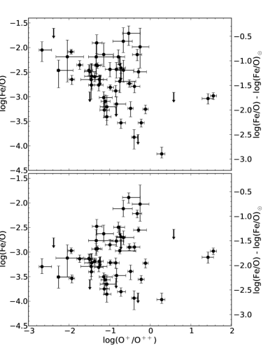
Figure 1.— Values of Fe/O (left axis) and the depletion factors for Fe/O ($[\mbox{Fe/O}]=\log(\mbox{Fe/O})-\log(\mbox{Fe/O})_{\odot}$, right axis) as a function of the degree of ionization for all the PNe. The upper panel shows the values obtained from equation (2) whereas the bottom panel shows the ones obtained with equations (3) or (4).

The right axis in Figure 1 shows estimates of the depletion factors for Fe/O. The depletion of one particular element (X) is usually calculated as the difference between the observed and the expected values of X/H: $[\mbox{X}/\mbox{H}]=\log(\mbox{X/H})-\log(\mbox{X/H})_{\rm ref}$. However, we will use Fe/O instead of Fe/H to calculate depletion factors, since the intrinsic value of Fe/O is expected to show less variations from object to object than either Fe/H or O/H (Ramírez et al., 2007). In principle, we could use a different reference element, but oxygen abundances require small ionization correction factors in most objects and hence are the ones that can be determined in a more reliable way. We adopted the solar value of $\log(\mbox{Fe/O})_{\odot}=-1.27\pm 0.11$ (Lodders, 2010) as the expected abundance ratio for our objects. For the range of metallicities covered by our sample PNe, the stellar values of Fe/O are found to decrease from solar to 0.4–0.5 dex below solar in the Galaxy (Meléndez et al., 2006; Ramírez et al., 2007). This means that the halo PN DdDm 1, that has the lowest metallicity and the highest Fe/O abundance ratio in our sample, could have a depletion factor close or equal to zero (but its infrared spectrum shows the presence of silicates, see § 6).

We should also bear in mind that the oxygen atoms may be depleted into dust grains, and in such case our values of $[\mbox{Fe}/\mbox{O}]$ should be lowered by up to $\sim$0.15 dex if oxygen is trapped in oxides and silicates (Whittet, 2010). On the other hand, in Rodríguez & Delgado-Inglada (2011) we found that the oxygen abundances in a group of PNe from the solar neighborhood were systematically higher than the ones in nearby H II regions (calculated either from collisionally excited lines or recombination lines). We suggested that the difference could be due to oxygen depletion in organic refractory dust components, but another possible explanation for these overabundances is oxygen production in the PN progenitor stars, and if this production is important, it will change significantly the value of Fe/O. However, the amount of oxygen production by AGB stars is very uncertain and could be negligible (see the predictions of models by different authors in Karakas & Lattanzio, 2007). Thus, we present our results for Fe/O, but in what follows we will check that our results hold both for the Fe/O and Fe/H abundance ratios.

As we mentioned above, our ionization correction scheme provides three values for the iron abundance, and the real value of Fe/O for each object is expected to lie in the range defined by these three values. We can see from Figure 1 that iron abundances are better constrained for objects with a relatively low degree of ionization, $\log(\mbox{O}^{+}/\mbox{O}^{++})\gtrsim-1.0$, where the three values obtained with the different ICFs differ by less than 0.5 dex. The values of $\log(\mbox{Fe/O})$ in our sample range from $-4.5$ to $-1.7$, which are the most extreme upper and lower limits that we find. In the same way, the depletion factors [Fe/O] range from $-3.2$ for IC 418 to $-0.4$ for DdDm 1.

Even taking into account all the considerations mentioned above that could change the iron depletions factors shown in the right axes of Figure 1, we can conclude that a significant fraction of our sample PNe have more than $\sim 90\%$ of their iron atoms deposited into dust grains. In agreement with our previous findings in a smaller sample of PNe (Delgado-Inglada et al., 2009), the range of depletions is high, with differences reaching a factor of $\sim 100$. These differences can be related to the PNe ages or grain compositions, maybe reflecting different efficiencies of the grain formation and destruction processes, an issue that we will explore further in the following sections.

5. The C/O abundance ratios

As we mentioned in § 1, one can expect a correlation between the C/O abundance ratios and the type of dust grains present in PNe. Unfortunately, obtaining accurate values of C/O for PNe is not easy (see, e.g., Rola & Stasińska, 1994; Henry et al., 1996). The ionic abundances of carbon and oxygen can be derived from collisionally excited lines (CELs) or from recombination lines (RLs), and the abundances obtained with RLs are systematically higher than the ones derived from CELs, by factors that are around two for many PNe but can reach $\sim$70 (see Liu et al., 2006). The reason for this discrepancy is still a matter of debate and we do not know which lines lead to more representative abundances in PNe. The abundances derived from CELs are highly dependent on the electron temperature, but these lines are brighter than RLs and thus, more easily measured. On the other hand, RLs are weakly dependent on physical conditions, but they are faint and may suffer from other problems (see, e.g, Rodríguez & García-Rojas, 2010; Escalante et al., 2012).

One important source of uncertainties in the C/O values derived from CELs is the normalization between ultraviolet and optical fluxes since carbon lines are found in the ultraviolet range whereas oxygen lines are better measured in the optical range. This correction introduces uncertainties in the values of C/O, which are more severe for extended objects, where ultraviolet and optical observations may cover different regions of the nebula. One advantage of using RLs is that this issue does not arise, since they are observed in the optical range.

A further complication is introduced by the ICFs needed to account for unobserved ions and estimate the total abundances. For oxygen we have used here the equation proposed by Peimbert & Torres-Peimbert (1971) to correct for the contribution of O⁺³ to the total abundance. In the case of oxygen abundances based on RLs, only the O⁺⁺ abundances can be easily calculated, and we assume that the distribution of all ionization states is equal to the one inferred from CELs. As for carbon, one can apply the widely used correction scheme of Kingsburgh & Barlow (1994), consisting of several ICFs which are employed depending on the degree of ionization of the object and the detected ionization stages (up to four different ions can be observed in PNe: C⁺, C⁺⁺, C⁺³, and C⁺⁴), although certain cases are not covered by this scheme. Therefore, the correction scheme of Kingsburgh & Barlow (1994) produces an inhomogeneous determination of carbon abundance when applied to different objects.

The other method that is frequently adopted to calculate C/O is $\mbox{C}/\mbox{O}=\mbox{C}^{++}/\mbox{O}^{++}$. However, this ICF generally overestimates the value of C/O, especially in low ionization PNe (Delgado-Inglada et al., 2014). Here we calculate C/O in a homogeneous way using the ICF derived in Delgado-Inglada et al. (2014):

$$\frac{{\rm C}}{{\rm O}}=\frac{{\rm C}^{++}}{{\rm O}^{++}}(0.05+2.21\omega-2.77\omega^{2}+1.74\omega^{3}),$$ (5)

where $\omega=\mbox{O}^{++}/(\mbox{O}^{+}+\mbox{O}^{++})$. This ICF is valid in the range $0.05<\omega<0.97$. In this range, the ICF is expected to reproduce the values of C/O to within ${}^{+0.13}_{-0.09}$ dex. However, the C/O values derived for NGC 40 (with $\omega=0.03$), and for IC 3568, IC 5217, NGC 3242, NGC 5882, M3-32, NGC 7662 (all of them with $\omega>0.97$) are more uncertain. For NGC 40, we estimate a confidence interval of ${}^{+0.26}_{-1.0}$ dex; for the objects with the highest values of $\omega$, we estimate confidence intervals of ${}^{+0.26}_{-0.22}$ dex. These uncertainties will be taken into account in the forthcoming analysis.

The value of the ICF in equation (5) is close to 1 for most of our objects, where $\omega\gtrsim 0.8$, changing the C⁺⁺/O⁺⁺ ratio by less than 0.05 dex. However, in the low ionization PNe IC 418 and NGC 40, the differences between both estimates reach 0.9 dex.

We compared the values of C/O implied by the three different methods described above ($\mbox{C}/\mbox{O}=\mbox{C}^{++}/\mbox{O}^{++}$, the set of ICFs from Kingsburgh & Barlow 1994, and the ICF from Delgado-Inglada et al. 2014) and by the two types of lines we use (CELs or RLs). We find that the differences seem to be more related to whether we use CELs or RLs than to the correction scheme we apply. Hence we will restrict the forthcoming discussion to the values of C/O calculated with equation (5), derived either from RLs or from CELs.

5.1. C/O from CELs

The C⁺⁺ abundances were calculated from the fluxes of the C III] $\lambda 1908$ doublet (provided in the same papers we use for the optical fluxes, see Table 2) through the IRAF routine ionic using the values of $n_{\rm e}$ and $T_{\rm e}$[O III] listed in Table 2. Since the collision strengths for C⁺⁺, derived by Berrington et al. (1985), are available only for $T_{\rm e}$ $>12600$ K, we extrapolated them to lower temperatures in order to cover the $T_{\rm e}$ range found for our sample PNe. Table 5 shows the values we obtain for C⁺⁺/H⁺.

The highest differences between our values of $\rm{C}^{++}/\rm{H}^{+}$ and the ones in the papers listed in Table 2 are found for Hu 1-1 (0.35 dex) and IC 4406 (0.23 dex). For the other PNe the differences are lower than 0.15 dex. These disagreements are due to the different physical conditions adopted in the calculations, except for IC 4406, for which the value given in Tsamis et al. (2003) is a typo, and their corrected value agrees with the one we derive (Y. Tsamis, private communication).

Using the values of O⁺⁺ from Table 2, we calculate the C/O values listed in the third column of Table 5. Because these values are based on CELs located in the optical ([O III] $\lambda\lambda 4959,5007$) and in the ultraviolet (C III] $\lambda 1908$), there are several important sources of uncertainty associated to them, namely, the adopted $T_{\rm e}$, the extinction correction, the normalization between ultraviolet and optical fluxes, and the aperture correction in extended nebulae. The uncertainties associated with the normalization of optical and ultraviolet fluxes are difficult to quantify. The other sources of uncertainty are discussed below.

The correction for interstellar extinction is important, and the extinction law for the bulge PNe, needed for some of our sample objects, is uncertain (see, e.g., Liu et al., 2001; Wang & Liu, 2007, and references therein). Even a small error in the extinction coefficient, $\sigma\{c(\mbox{H}\beta)\}=0.1$, introduces an uncertainty of $\sim 0.1$ dex in the intensity ratio of the C III] $\lambda$1908 and [O III] $\lambda$4959 lines. However, the main effect of an error in the extinction coefficient will occur through its impact on the derived temperature. The determination of an accurate value of $T_{\rm e}$ is a critical factor in obtaining reliable ionic abundances from CELs, and the emissivities of ultraviolet CELs are more dependent on $T_{\rm e}$ than those of optical CELs. As an example, consider an error of 500 K, which can arise easily from errors in the extinction correction, the flux calibration or the line measurements that will not necessarily appear in the quoted line intensity errors. At $T_{\rm e}$ $=10000$ K, this variation introduces a change of $0.18$ dex in C⁺⁺/H⁺ and a change of $0.07$ dex in O⁺⁺/H⁺; the final effect in the C⁺⁺/O⁺⁺ ratio will be around 0.1 dex.

Aperture corrections are needed in those nebulae that are more extended than the aperture of the International Ultraviolet Explorer ($\sim 10\times 20$ arsec²), or that were observed in the optical with a long slit at a single position (as opposed to a long slit scanning the whole object). The scale factors applied by the different authors in our sample PNe go up to 13, with NGC 6720 (angular diameter of 76 arcsec) the PN with the highest aperture correction (Liu et al., 2004a). We use here the ultraviolet fluxes provided by the different authors, already scaled and normalized by them. The uncertainties related to this procedure are difficult to estimate, but might reach a factor of 2–3 for objects like NGC 6720.

Table 5 shows the C⁺⁺ abundances and the values of C/O based on CELs and the ICF of equation (5). We only present in this table the uncertainties associated with the final values of C/O. We consider an uncertainty of 0.2 dex in $(\mbox{C}^{++}/\mbox{O}^{++})_{\rm CELs}$, based on the discussion above (it could be higher for some objects, such as extended nebulae with important aperture corrections), which is added quadratically to the uncertainty in the ICF computed from equations (40) and (41) in Delgado-Inglada et al. (2014).

Table 5Ionic abundances: {X⁺ⁱ} = 12 + $\log$ (X⁺ⁱ/H⁺) and $\log$(C/O) values from CELs and RLs

PN	CELs		RLs
	{C++}	$\log$(C/O)	{C++}	{O++}	$\log$(C/O)
Cn 1-5	9.04	$0.28^{+0.20}_{-0.22}$	9.08	8.90	$0.09^{+0.05}_{-0.10}$
Cn 3-1	$\ldots$	$\ldots$	8.05	$\ldots$	$\ldots$
DdDm 1	6.78	$-1.16^{+0.20}_{-0.22}$	$\ldots$	8.43	$\ldots$
H 1-41	$\ldots$	$\ldots$	8.57	9.18	$-0.56^{+0.09}_{-0.10}$
H 1-42	7.61	$-0.86\pm 0.22$	8.34	8.92	$-0.52\pm 0.10$
H 1-50	7.82	$-0.76^{+0.21}_{-0.22}$	8.63	9.05	$-0.38^{+0.09}_{-0.10}$
Hu 1-1	$\ldots$	$\ldots$	8.94	8.54	$0.33^{+0.05}_{-0.10}$
Hu 2-1	8.53	$0.34^{+0.21}_{-0.22}$	8.62	8.71	$-0.09^{+0.07}_{-0.10}$
IC 418	8.35	$0.04^{+0.21}_{-0.22}$	8.73	8.21	$0.26^{+0.06}_{-0.10}$
IC 1747	9.04	$0.55\pm 0.22$	9.09	8.76	$0.39\pm 0.10$
IC 2165	8.28	$0.24\pm 0.22$	8.53	8.63	$-0.04^{+0.09}_{-0.10}$
IC 3568	8.05	$-0.22\pm 0.22$	8.49	8.75	$-0.17\pm 0.10$
IC 4191	$\ldots$	$\ldots$	8.72	9.07	$-0.30^{+0.09}_{-0.10}$
IC 4406	8.57	$-0.10^{+0.20}_{-0.22}$	8.89	8.89	$-0.09^{+0.05}_{-0.10}$
IC 4593	$\ldots$	$\ldots$	8.63	8.65	$0.02^{+0.09}_{-0.10}$
IC 4699	8.00	$-0.32\pm 0.22$	8.72	9.15	$-0.35^{+0.11}_{-0.10}$
IC 4846	7.86	$-0.55\pm 0.22$	8.16	8.76	$-0.52\pm 0.10$
IC 5217	8.26	$-0.29\pm 0.22$	8.36	8.65	$-0.20\pm 0.10$
JnEr 1	$\ldots$	$\ldots$	$\ldots$	$\ldots$	$\ldots$
M 1-20	$\ldots$	$\ldots$	8.66	8.63	$0.08^{+0.08}_{-0.10}$
M 1-42	7.92	$-0.44^{+0.21}_{-0.22}$	9.38	9.63	$-0.25^{+0.07}_{-0.10}$
M 1-73	$\ldots$	$\ldots$	8.73	9.00	$-0.34^{+0.05}_{-0.10}$
M 2-4	$\ldots$	$\ldots$	8.50	8.89	$-0.37^{+0.07}_{-0.10}$
M 2-6	$\ldots$	$\ldots$	7.90	8.62	$-0.74^{+0.06}_{-0.10}$
M 2-27	$\ldots$	$\ldots$	8.84	9.37	$-0.50^{+0.08}_{-0.10}$
M 2-31	$\ldots$	$\ldots$	8.79	$\ldots$	$\ldots$
M 2-33	8.59	$-0.02\pm 0.22$	8.30	9.04	$-0.68^{+0.07}_{-0.10}$
M 2-36	8.65	$-0.03^{+0.21}_{-0.22}$	9.36	9.51	$-0.11^{+0.08}_{-0.10}$
M 2-42	$\ldots$	$\ldots$	$\ldots$	9.60	$\ldots$
M 3-7	$\ldots$	$\ldots$	$\ldots$	9.42	$\ldots$
M 3-29	$\ldots$	$\ldots$	8.51	9.25	$-0.75^{+0.07}_{-0.10}$
M 3-32	8.42	$-0.06\pm 0.22$	9.55	9.74	$-0.10^{+011}_{-0.10}$
MyCn 18	$\ldots$	$\ldots$	8.36	8.81	$-0.47^{+0.07}_{-0.10}$
NGC 40	8.01	$-0.02^{+0.24}_{-0.22}$	8.81	8.61	$-0.76^{+0.14}_{-0.10}$
NGC 2392	7.69	$-0.39^{+0.21}_{-0.22}$	$\ldots$	9.81	$\ldots$
NGC 3132	8.18	$-0.47^{+0.20}_{-0.22}$	8.82	8.80	$-0.11^{+0.05}_{-0.10}$
NGC 3242	8.04	$-0.28\pm 0.22$	8.79	8.78	$0.09^{+0.09}_{-0.10}$
NGC 3587	$\ldots$	$\ldots$	8.36	9.38	$-1.13^{+0.05}_{-0.10}$
NGC 3918	8.36	$-0.07^{+0.21}_{-0.22}$	8.70	8.75	$-0.06^{+0.07}_{-0.10}$
NGC 5882	8.11	$-0.46\pm 0.22$	8.58	8.93	$-0.27\pm 0.10$
NGC 6153	8.38	$-0.16\pm 0.22$	9.35	9.51	$-0.09\pm 0.10$
NGC 6210	7.87	$-0.60\pm 0.22$	8.80	9.53	$-0.66\pm 0.10$
NGC 6439	8.32	$-0.24^{+0.21}_{-0.22}$	8.99	9.21	$-0.21^{+0.07}_{-0.10}$
NGC 6543	8.48	$-0.19\pm 0.22$	8.76	9.07	$-0.24\pm 0.10$
NGC 6565	8.29	$-0.32^{+0.20}_{-0.22}$	8.65	8.85	$-0.25^{+0.05}_{-0.10}$
NGC 6572	8.77	$0.25^{+0.21}_{-0.22}$	8.69	8.71	$0.03^{+0.09}_{-0.10}$
NGC 6620	8.16	$-0.58^{+0.20}_{-0.22}$	8.94	9.24	$-0.36^{+0.05}_{-0.10}$
NGC 6720	8.38	$-0.19^{+0.20}_{-0.22}$	8.94	8.90	$-0.08^{+0.05}_{-0.10}$
NGC 6741	8.40	$-0.09^{+0.20}_{-0.22}$	8.79	8.74	$-0.04^{+0.05}_{-0.10}$
NGC 6803	8.24	$-0.33\pm 0.22$	8.79	9.05	$-0.21^{+0.09}_{-0.10}$
NGC 6818	8.17	$-0.14\pm 0.22$	8.66	8.57	$0.12^{+0.08}_{-0.10}$
NGC 6826	8.40	$-0.03\pm 0.22$	8.73	8.92	$-0.11\pm 0.10$
NGC 6884	8.45	$-0.02\pm 0.22$	8.87	8.98	$-0.05^{+0.09}_{-0.10}$
NGC 7026	8.33	$-0.26^{+0.21}_{-0.22}$	8.93	9.07	$-0.13^{+0.07}_{-0.10}$
NGC 7662	7.99	$-0.15^{+0.21}_{-0.22}$	8.67	8.58	$0.17\pm 0.10$
Vy 2-1	8.61	$-0.11^{+0.21}_{-0.22}$	8.62	8.98	$-0.34^{+0.07}_{-0.10}$

5.2. C/O from RLs

C II and O II RLs can be measured in the optical range and do not suffer from many of the uncertainties discussed above. Therefore, these lines will provide better estimates of the C/O abundance ratio, or they will do so if they can be considered to sample the abundances of the nebular gas. For example, these emission lines might not be representative of the nebular abundances if they arise mostly from metal-rich inclusions, whose existence in PNe has been postulated to explain the discrepant abundances implied by CELs and RLs (see, e.g., Liu et al., 2004a).

The C⁺⁺/H⁺ and O⁺⁺/H⁺ abundance ratios implied by RLs are derived for all objects with available measurements of the required RLs using the values of $n_{\rm e}$ and $T_{\rm e}$[O III] in Table 2 and the effective recombination coefficients for H$\beta$ of Storey & Hummer (1995). The C⁺⁺ abundances are calculated using the C II $\lambda$4267 line and the case B effective recombination coefficients of Davey et al. (2000). The O⁺⁺ abundances are computed from the total intensity of multiplet 1 of O II and the recombination coefficients of Storey (1994). The multiplet intensity was corrected for the contribution of undetected lines with the formulae derived by Peimbert et al. (2005). Typical errors in C⁺⁺/H⁺ and O⁺⁺/H⁺ arising from errors in the line intensities are $\pm 0.02$ dex and $\pm 0.06$ dex, respectively. Final errors in C⁺⁺/O⁺⁺ due to errors in the line intensities are around $\pm 0.06$ dex. If we also consider the uncertainties in the ICF, as explained in § 5.1, we obtain the final uncertainties presented in Table 5 together with the ionic abundances of C⁺⁺ and O⁺⁺ obtained from RLs.

We found differences between our values and the ones in the reference papers that are in general lower than 0.06 dex but reach 0.17 dex for some nebulae. The highest differences are found for H 1-42 (with a difference of 0.32 dex in the value of C⁺⁺/H⁺), M 2-42 (0.56 dex in O⁺⁺/H⁺), and M 3-29 (0.49 dex in O⁺⁺/H⁺) and are not due to differences in the physical conditions used in the calculations. We do not know the reasons for these discrepancies, but they do not affect our conclusions, since we do not have information about the types of grains present in H 1-42 and M 3-29, and we cannot calculate the C/O abundance ratio in M 2-42. Hence, these PNe are not included in the forthcoming analysis.

Figure 2 shows a comparison between the values of C/O obtained from CELs and RLs in those PNe where both types of lines are observed. We also plot in the figure the error bars associated with this abundance ratio for each object. The error bars take into account both the uncertainties in the line intensity ratios ($\pm 0.2$ dex for the values derived from CELs and $\pm 0.06$ dex for the ones derived from RLs) and the uncertainties in the ICF. Although there is general agreement between these two abundance ratios, a result previously found in several studies (see Liu et al., 2004a, and references therein), the differences are high for some objects. The highest differences reach $\sim 0.7$ dex and are found for NGC 40 and M 2-33. NGC 40 is an extended PN (diameter of around 48 arcsec) with a Wolf-Rayet central star, thus, an incorrect aperture correction and/or contamination of the ultraviolet line fluxes with stellar winds could explain the discrepancy. M 2-33 is smaller (with a diameter of around 5.8 arcsec) and thus, we expect that the scaling of optical and ultraviolet observations is not that critical. The discrepancy could also be explained if the $T_{\rm e}$ is underestimated by $\sim 3000$ K, but we do not expect such a large error in $T_{\rm e}$. We have explored if the differences between the ionic abundance ratios derived from CELs and RLs are related to parameters such as $T_{\rm e}$[O III], $n_{\rm e}$, the extinction coefficient, the nebular size, the type of dust, the abundance discrepancy factor, or the $T_{\rm e}$ deduced from the H I recombination continuum Balmer discontinuity, but we do not find any obvious correlation.

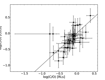
Figure 2.— Comparison of C/O = C⁺⁺/O⁺⁺ values derived from CELs and from RLs. The error bars represent typical errors as explained in the text. The line shows where the values of C/O are equal.

As we mentioned above, the C/O abundance ratios in PNe tell us whether the ionized gas is carbon rich or oxygen rich. We find that both CELs and RLs imply that 20% of the PNe are C–rich. Most of the PNe in our sample seem to be O-rich objects. According to theoretical models (see, e.g., Marigo et al., 2003), these PNe evolve either from the lowest mass progenitors (masses below 1.5 M_⊙) or from the highest mass progenitors (above 4–5 M_⊙), although the details depend on the metallicity and on the model assumptions.

6. Dust features from infrared spectra

We used the archive of the Infrared Spectrograph (IRS; Houck et al. 2004), on board the Spitzer Space Telescope (Werner et al., 2004), to download the spectra available for our sample PNe. We decided to look for the following dust features: polycyclic aromatic hydrocarbons (PAHs), the broad features around 11 and 30 $\mu$m (usually associated with SiC and MgS, respectively), amorphous silicates, and crystalline silicates. We restricted the analysis to these features because they are relatively easy to identify and are, in principle, reliably associated with either a carbon-rich or an oxygen-rich environment (we will come back to this point later). A detailed analysis of all the dust features present in the PNe is beyond the scope of this paper. We also compiled dust identifications from the literature, mainly from spectra of the Infrared Space Observatory (ISO; Kessler et al. 1996). The results are summarized in Table 6 and are discussed below.

Table 6Compilation of dust features, range of Fe/O values: {Fe/O} = $\log$(Fe/O), and $\log$(C/O) values.

Object	$\Delta${Fe/O}	$\log$(C/O)	PAHs	SiC	30 $\mu$m	Amorphous	Crystalline	Source
		CELs/RLs				silicates	silicates
Cn 1-5	$[-2.4,-2.1]$	$+0.28$/$+0.09$	$\surd$	$\times$	$\times$	$\times$	$\surd$	ISO (1), Spitzer (2,3), UKIRT (7)
DdDm 1	$[-2.0,-1.7]$	$-1.16$/$\ldots$	$\times$	$\times$	$\times$	$\surd$	$\surd$	Spitzer (3,4)
H 1-50	$[-3.6,-3.1]$	$+0.34$/$-0.09$	$\surd$?	$\times$	$\times$	$\surd$	$\surd$	Spitzer (2,3)
Hu 2-1	$[-3.0,-2.7]$	$+0.34$/$-0.09$	$\surd$	$\surd$	$\ldots$	$\times$	$\ldots$	ISO (1), Spitzer (3), UKIRT (6)
IC 418	$[-4.5,-4.0]$	$+0.04$/$+0.26$	$\surd$	$\surd$	$\surd$	$\times$	$\ldots$	ISO (1, 5), Spitzer (3), UKIRT (6)
IC 2165	$[-2.9,-2.4]$	$+0.24$/$-0.04$	$\times$	$\surd$?	$\ldots$	$\times$	$\ldots$	Spitzer (3), UKIRT (6)
IC 3568	$[-3.3,-2.0]$	$-0.22$/$-0.17$	$\times$	$\ldots$	$\ldots$	$\ldots$	$\ldots$	ISO (1)
IC 4406	$<-3.8$	$-0.10$/$-0.09$	$\times$	$\ldots$	$\ldots$	$\ldots$	$\ldots$	ISO (1)
IC 4846	$[-3.3,-2.6]$	$-0.55$/$-0.52$	$\times$	$\times$	$\times$	$\surd$?	$\times$?	Spitzer (3)
M 1-20	$[-3.6,-3.2]$	$\hskip 5.97527pt\ldots$/$+0.08$	$\surd$	$\surd$	$\surd$	$\times$	$\times$	Spitzer (2,3,8), UKIRT (7)
M 1-42	$<-2.2$	$-0.44$/$-0.25$	$\surd$	$\times$	$\times$	$\times$	$\surd$	ISO (1), Spitzer (3)
M 2-27	$[-2.8,-2.4]$	$\hskip 5.97527pt\ldots$/$-0.50$	$\surd$	$\times$	$\times$	$\times$	$\surd$	Spitzer (2,3)
M 2-31	$[-2.5,-1.9]$	$\hskip 5.97527pt\ldots$/$\ldots$	$\surd$	$\times$	$\times$	$\times$	$\surd$	Spitzer (3,9)
M 2-36	$[-3.9,-3.4]$	$-0.03$/$-0.11$	$\times$	$\ldots$	$\ldots$	$\ldots$	$\ldots$	ISO (1)
M 2-42	$[-2.9,-2.4]$	$\hskip 5.97527pt\ldots$/$\ldots$	$\times$	$\times$	$\times$	$\times$	$\surd$	Spitzer (3)
MyCn 18	$[-2.7,-2.4]$	$\hskip 5.97527pt\ldots$/$-0.47$	$\surd$	$\times$	$\times$	$\surd$	$\surd$	Spitzer (3)
NGC 40	$[-3.3,-3.0]$	$-0.02$/$-0.76$	$\surd$	$\times$	$\surd$	$\times$	$\times$	ISO (1, 5), Spitzer (3)
NGC 2392	$[-2.2,-1.9]$	$-0.39$/$\ldots$	$\times$	$\times$	$\times$	$\times$	$\times$	Spitzer (3)
NGC 3132	$[-3.6,-3.2]$	$-0.47$/$-0.11$	$\times$	$\times$	$\times$	$\times$	$\surd$	Spitzer (3)
NGC 3242	$[-3.5,-2.6]$	$-0.28$/$+0.09$	$\times$	$\times$	$\surd$	$\times$	$\times$	Spitzer (3)
NGC 3918	$[-3.8,-3.5]$	$-0.07$/$-0.06$	$\times$	$\times$	$\surd$	$\times$	$\ldots$	ISO (1, 5, 10), Spitzer (3)
NGC 6153	$[-3.4,-2.8]$	$-0.16$/$-0.09$	$\times$	$\ldots$	$\ldots$	$\surd$?	$\times$?	ISO (1, 10)
NGC 6210	$[-3.3,-2.8]$	$-0.60$/$-0.66$	$\times$	$\times$	$\times$	$\times$?	$\surd$	ISO (1), Spitzer (3)
NGC 6439	$[-3.2,-2.9]$	$-0.24$/$-0.21$	$\surd$?	$\times$	$\times$	$\times$	$\surd$	Spitzer (3)
NGC 6543	$[-3.1,-2.5]$	$-0.19$/$-0.24$	$\times$	$\ldots$	$\ldots$	$\surd$	$\surd$	ISO (1, 10)
NGC 6572	$[-3.5,-3.0]$	$+0.25$/$+0.03$	$\times$	$\surd$?	$\ldots$	$\times$	$\times$	ISO (1), UKIRT (6)
NGC 6720	$[-3.8,-3.5]$	$-0.19$/$-0.08$	$\times$	$\times$	$\ldots$	$\times$	$\ldots$	ISO (1), Spitzer (3)
NGC 6741	$[-2.8,-2.5]$	$-0.09$/$-0.04$	$\surd$	$\times$	$\ldots$	$\times$	$\ldots$	ISO (1), Spitzer (3), UKIRT (6)
NGC 6818	$[-3.2,-2.8]$	$-0.14$/$+0.12$	$\times$	$\times$	$\times$	$\times$	$\times$?	Spitzer (3)
NGC 6826	$[-3.1,-2.5]$	$-0.03$/$-0.11$	$\times$	$\times$	$\surd$	$\times$	$\ldots$	ISO (1, 5), Spitzer (3)
NGC 6884	$[-3.2,-2.6]$	$-0.02$/$-0.05$	$\surd$	$\times$	$\ldots$	$\times$	$\ldots$	ISO (1), Spitzer (3)
NGC 7026	$<-3.2$	$-0.26$/$-0.13$	$\surd$	$\times$	$\times$	$\times$	$\surd$	Spitzer (3)
NGC 7662	$[-3.0,-2.1]$	$-0.15$/$+0.17$	$\times$	$\times$	$\ldots$	$\times$	$\ldots$	ISO (1), Spitzer (3)

References. — (1) Cohen & Barlow (2005), (2) Perea-Calderón et al. (2009), (3) this work, (4) Henry et al. (2008), (5) Hony et al. (2002), (6) Casassus et al. (2001a), (7) Casassus et al. (2001b), (8) García-Hernández et al. (2010), (9) Gutenkunst et al. (2008), (10) Bernard-Salas & Tielens (2005), (11) Stanghellini et al. (2012)

6.1. Data from Spitzer

We found Spitzer IRS spectra for 27 PNe of our sample (we excluded the very noisy spectra of JnEr 1 and NGC 3587). The data belong to the following observing programs: ID 45 (PI: T. Roellig), ID 93 (PI: D. Cruikshank), ID 1406 (PI: L. Armus), ID 1427 (calibration program), ID 20049 (PI: K. Kwitter), ID 30285, 40115 (PI: G. Fazio), ID 30430, 40536 (PI: H. Dinnerstein), ID 30550 (PI: J. R. Houck), ID 3633 (PI: M. Bobrowsky), and ID 50261 (PI: L. Stanghellini). The Spitzer spectra of Cn 1-5, DdDm 1, H 1-50, IC 4846, M 1-20, M 2-27, M 2-42, M 2-31, and MyCn 18 have been studied already in several works (Perea-Calderón et al., 2009; Gutenkunst et al., 2008; Henry et al., 2008; Stanghellini et al., 2012), where some of the dust features in these objects are identified.

The PNe were observed with at least one of the four different modules of IRS (SL, LL, SH, and LH) and, therefore, the wavelength coverage and the spectral resolution are not the same for all the nebulae. Each module is named by its wavelength coverage and resolution as Short-Low (SL, covering the range 5.2–14.5 $\mu$m with a spectral resolution $\lambda$/$\Delta\lambda$ = 64–128), Long-Low (LL: 14.0–38 µm and the same spectral resolution as SL), Short-High (SH: 9.9–19.6 $\mu$m and $\lambda$/$\Delta\lambda$ $\sim$ 600), and Long-High (LH: 18.7–37.2 $\mu$m and the same spectral resolution as SH). We used the observations performed in the staring mode in which the object is placed at two different positions (nods) in the slit.

We retrieved the data from the Spitzer/IRS archive and we reduced them following the usual steps. We started the reduction from the Base Calibrated Data (BCD). First, we used the IDL procedure doall_coads to produce a single coadded image for each nod position and module separately. Each of the low-resolution modules contains two slits; when one of them is observing the source, the other one is off-source. We used the off-source spectra to subtract the background in the on-source spectra. For the high-resolution modules, extra sky images are needed to remove this contribution in the source spectra. In some cases, there were no available images to remove the sky background, but this is not important for our identification purposes. Rogue pixels were removed with the irsclean tool. The spectra for each nod position was wavelength and flux calibrated, and extracted with the Spitzer IRS Custom Extractor (SPICE) using one of the two available extractions: point-source aperture or full-slit extraction, depending on the size of the PNe. Finally, we used the Spectroscopic Modeling Analysis and Reduction Tool (SMART, Higdon et al. 2004; Lebouteiller et al. 2010) to manually eliminate bad pixels, jumps, and to combine and merge into one final spectra the observations of each module. High-resolution spectra were smoothed using a box-car algorithm (of widths 0.06 $\mu$m and 0.08 $\mu$m for the SH and LH modules, respectively) to slightly lower the noise without losing information about the dust features.

Different regions of the final Spitzer/IRS spectra for the 27 sample PNe are shown in Figures 3–6. For the convenience of the reader, we display all the Spitzer spectra available for our objects, although some of them have already been published, and some of the features of interest have been identified in the works we mentioned above. A total of 18 PNe have observations for the whole IRS spectral range, 5–37 $\mu$m, where many dust features can be observed (Figs. 4 and 5). The other nebulae do not have data for the full spectral range that can be covered with Spitzer/IRS. On the other hand, some objects have wavelength ranges covered at both high and low spectral resolutions. In such cases, we show the spectra where the dust emission features can be seen more clearly.

6.2. Identification of dust features

6.2.1 C-rich features: SiC, the 30 $\mu$m feature, and PAHs

Using the IRS spectra, we identify the broad feature around 11.3 µm, associated with SiC grains, in Hu 2-1, IC 418, and M 1-20 (Figs. 3–4). This feature was already detected by Casassus et al. (2001a, b) and Cohen & Barlow (2005) in UKIRT and ISO spectra of these three PNe, and also in IC 2165 and NGC 6572. In the last two PNe, the feature is not as evident as for the other objects. In the case of IC 2165, there are Spitzer/IRS spectra, and we do not see clear evidence of the feature (Fig. 3). Therefore, we label the identification as doubtful in this PNe.

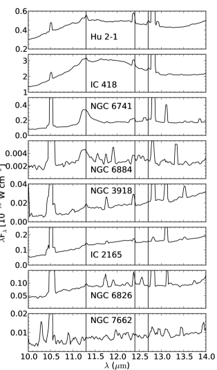
Figure 3.— Spitzer/IRS spectra showing PAH and/or SiC features. The solid lines are at the wavelengths of the usual peak intensities of the PAH features at 11.3, 12.4, and 12.7 $\mu$m. The spectra available for these PNe do not cover the same range as the ones for the objects shown in Figures 4 and 5.

The 30 $\mu$m feature, often attributed to MgS grains, is present in the spectra of NGC 3242 and M 1-20 (see Fig. 5). Besides, Hony et al. (2002) detected this feature in ISO spectra of IC 418, NGC 40, NGC 3918, and NGC 6826. We do not observe the feature in NGC 40, but this could be due to the different areas observed by ISO ($\sim$ 440 arcsec², covering almost the whole nebula) and Spitzer ($\sim$ 248 arcsec²).

Figure 4.— Spitzer/IRS spectra showing PAH features. Thin vertical lines represent the usual peak intensity of the features at 8.6, 11.3, 12.4, and 12.7 $\mu$m, whereas shaded areas show the range of variation for peak intensity of the features at 6.2 and 7.7 $\mu$m. The PNe are ordered as in figure 5.

Figure 5.— Spitzer/IRS spectra showing crystalline silicate complexes around 23, 28, and 33 $\mu$m (grey rectangles), amorphous silicates, SiC, and the broad feature at 30 $\mu$m. The PNe are ordered according to the prominence of their crystalline silicate features.

There are PAH features in the IRS spectra of 12 of the 27 PNe with available data (see Figs. 3–4), and we cannot rule out their presence in at least 2 of the other PNe. Some of the PNe would require deeper spectra or a higher spectral resolution to reach more definitive conclusions. As an example, Cohen & Barlow (2005) did not find PAHs in M 1-42 using ISO observations, but we think that the Spitzer spectra of this nebula shows evidence of these features (see Fig. 4). For this nebula, a higher spectral resolution would show the presence or absence of PAHs more clearly.

The detection of PAHs is not clear in some nebulae, in particular those with spectra of low spectral resolution, because of contamination with emission lines (see Fig. 6 for some identifications). We see that in those PNe where PAHs are more conspicuous, such as NGC 40 and Cn 1-5 (Fig. 4), the broad feature at 11.3 $\mu$m is the PAH feature most easily seen. Hence we used the presence of this broad feature as the main criterion for the detection of PAHs.

Originally, PAHs were thought to appear only in those dust forming sources that are carbon-rich (Whittet, 2003), but in recent years these molecules have also been observed in oxygen-rich AGB and post-AGB stars, and in oxygen-rich PNe (see, e.g., Jura et al., 2006; Cerrigone et al., 2009; Guzmán-Ramírez et al., 2011; Gielen et al., 2011). These so-called mixed-chemistry PNe show PAHs and crystalline silicate features together in their infrared spectra (see e.g. Waters et al., 1998; Cohen et al., 1999). We will come back to this issue in § 6.2.2.

Figure 6 shows the 6–14 $\mu$m IRS spectra of NGC 6720, which has observations at three different locations. The upper panel shows the spectrum for a region that includes part of the outer halo of the nebula; the middle panel shows the spectrum for an aperture that crosses the halo; and the lower panel shows the spectrum for an aperture that crosses the bright region close to the center of the nebula. We do not see evidence for PAHs, SiC, nor amorphous silicates.

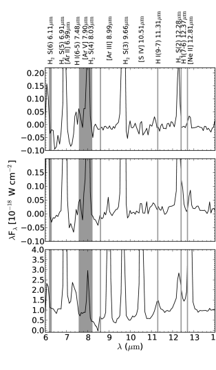
Figure 6.— Spitzer/IRS spectra for three different positions in NGC 6720. Grey lines and rectangles represent the usual peak intensity of the PAH features at 8.6, 11.3, 12.4, and 12.7 $\mu$m, and the range of variation for peak intensity of the features at 6.2 and 7.7 $\mu$m.

6.2.2 O-rich features: amorphous and crystalline silicates

We observe the broad features associated with amorphous silicates in 3–5 PNe of the 27 PNe with IRS/Spitzer spectra in the adequate wavelength range (see Figs. 4 and 5). DdDm 1, MyCn 18, and H 1-50 show the feature at 9.7 $\mu$m and some indication of the 18 $\mu$m feature. We cannot rule out the presence of these features in IC 4846 and NGC 6210. Some PNe, like NGC 40, NGC 2392, and NGC 6210, show a small bump around 17–18 $\mu$m, but this feature is likely to be related with problems in the overlap of the SH and LH spectra. Finally, Bernard-Salas & Tielens (2005) identified amorphous silicates in the ISO spectra of NGC 6543 and, probably, in NGC 6153.

We also identify the crystalline silicate features around 23$\mu$m, 27$\mu$m, and 33 $\mu$m in the IRS spectra of 12 PNe from the sample. We cannot rule out the presence of crystalline silicates in IC 4846 and NGC 6818 due to the low resolution or poor signal-to-noise ratio of their spectra. Bernard-Salas & Tielens (2005) used ISO spectra and detected crystalline silicates in NGC 6543, whereas they could not rule out their presence in NGC 6153. Therefore, 13–16 nebulae from the 21 PNe with available spectra in the required wavelength range show crystalline silicates. The three PNe with amorphous silicates also show crystalline silicates.

Six out of the thirteen PNe that show silicate features belong to the mixed-chemistry class, objects that show both silicates and PAHs. Several scenarios have been proposed to explain the simultaneous presence of silicates and PAHs in PNe (see, e.g., Perea-Calderón et al., 2009). One of the preferred explanations is that the silicates were formed and ejected before the star experienced the third dredge-up, when it was still O-rich, whereas PAHs form later (Waters et al., 1998). According to this scenario, silicates are located in a O-rich disk/torus while PAHs occupy a more recent C-rich outflow. This could explain the mixed chemistry of Cn 1-5, where me measure C/O $>1$. However, this explanation is not valid for stars that remain O-rich during their whole evolution, either because the third dredge-up does not occur due to their low initial masses or because the effect of the third dredge-up is counteracted by the hot bottom burning process. In these PNe, it might apply the explanation proposed by Guzmán-Ramírez et al. (2011), in which the PAHs form in an O-rich and dense torus after the CO molecules are dissociated.

7. Discussion

The values of $12+\log(\mbox{O}/\mbox{H})$ in our sample of PNe go from 8.02 (for the halo PN DdDm 1) to 8.88 (for NGC 6620). If we consider the values of O/H found for the PNe that have different dust features, they cover the ranges: 8.26–8.87 (PAHs), 8.26–8.68 (SiC or 30 $\mu$m feature), 8.02–8.87 (silicates), and 8.45–8.87 (mixed-chemistry objects: silicates and PAHs). Thus the sample PNe with silicate dust grains seem to arise from a broad population that includes the halo PN, DdDm 1, PNe from the Galactic disk, and objects that might belong to the bulge, like H 1-50 and M 2-31 (Wang & Liu, 2007). Our PNe with SiC and the 30 $\mu$m feature seem to arise from a more homogeneous population in the Galactic disk; only one of them, M 1-20, might belong to the bulge. This agrees with the results of Stanghellini et al. (2012), who found that six of their compact Galactic PNe with C-rich dust features, for which they could estimate the dust temperature, follow a well defined sequence in their plots of dust temperature versus infrared luminosity or physical radii. Stanghellini et al. (2012) conclude that this is an evolutionary sequence and that the progenitors of these PNe covered a narrow range in initial mass and metallicity. The high oxygen abundances found for the mixed-chemistry PNe also agree with the results of Stanghellini et al. (2012), since they found that these nebulae are concentrated towards the Galactic center and are absent from the Magellanic Clouds.

The range of iron depletions we find in our sample of PNe covers about two orders of magnitude, suggesting differences in the formation and evolution of dust grains from one PN to another. As in Delgado-Inglada et al. (2009), we explored possible correlations between the iron depletions and different nebular and stellar parameters such as the electron density, the nebular radius, the surface brightness, the effective temperature of the central star, or the nebular morphology. In agreement with Delgado-Inglada et al. (2009), we do not find any obvious correlation. We investigate here if this large range of iron depletions is related to the type of dust grains found in the PN (i.e., C-rich or O-rich dust grains) or to the dominant chemistry present in the ionized gas (i.e., if the computed C/O ratio is lower or greater than one). In Figure 7 we display the values of Fe/O and the depletion factors for Fe/O as a function of the C/O abundance ratios, derived from CELs and RLs, for all the PNe in our sample with available data. Note that the sample PNe can have two, one, or no values for C/O (depending on whether the required CELs and RLs are measured or not) and hence not all the PNe in Table 3 appear in Figure 7, and some objects only appear in the panels at the right (left). We present the results for the values of Fe/O derived with equations (3) and (4), but the values of Fe/O implied by equation (2) lead to similar results.

Figure 7.— Values of Fe/O (left axis) and the depletion factors for Fe/O ($[\mbox{Fe/O}]=\log(\mbox{Fe/O})-\log(\mbox{Fe/O})_{\odot}$, right axis) as a function of the C/O abundance ratios obtained from CELs (right panels) and RLs (left panels) for all the PNe with available data. We use the symbols identified in each panel to mark those PNe with detections and non-detections of different infrared dust features.
(A color version of this figure is available in the online journal.)

We also identify in Figure 7 the PNe showing dust features in their infrared spectra, as well as those with doubtful or no detection of dust features. Note that, given the uncertainties related to the calculation of C/O from emission lines, the type of dust grains (O-rich or C-rich excluding PAHs) might provide better information on whether the intrinsic value of C/O in the nebular gas is above 1 or not (unless grain components like SiC can form in slightly O-rich conditions, see Bond et al., 2010).

The upper panels of Figure 7 show the PAH identifications. The first studies on the relation between PAHs and the C/O abundance ratios found a trend of increasing strength of these features as C/O increases (Cohen & Barlow, 2005, and references therein), and it was suggested that these molecules are only present in PNe with C/O $>1$. Here we find some PNe with intense PAH features and low C/O ratios, such as NGC 7026 or NGC 6439. Besides, PAH emission is not restricted to PNe with C/O $>1$, in agreement with the idea that PAH molecules may form both in C-rich and O-rich environments (Guzmán-Ramírez et al., 2011). We also see from this figure that PNe with PAHs are distributed over the whole range of iron depletions, suggesting that the presence of these molecules has no direct relation with the highest and lowest iron depletions found in the ionized gas.

The middle panels of Figure 7 identify those PNe with SiC or the broad feature at 30 $\mu$m, usually associated with dust grains formed in a C-rich environment. Most of these PNe are located close to the region where C/O $>1$. NGC 40 has a C/O value from RLs that is not consistent within the errors with C/O $>1$, but its C/O value from CELs is consistent with C/O = 1. On the other hand, Bond et al. (2010) find in their simulations of terrestrial planet formation that solid SiC can form when the C/O ratio is above 0.8. In this case, the range of C/O ratios for nebulae with C-rich dust can be somewhat wider.

The lower panels of Figure 7 show the PNe with amorphous or crystalline silicates in their spectra. These dust features seem to be very common in our sample. All but one of those PNe with silicate features have values of C/O that are compatible with an O-rich environment. Cn 1-5 is the exception, showing silicates with a C/O value clearly above one, regardless of what lines are used in the abundance determination and regardless of the adopted ICF. One possible explanation for this is that the C⁺⁺/O⁺⁺ values derived from CELs and RLs are seriously wrong for this nebula. Another option, already mentioned in § 6, is that the computed C/O value in the ionized gas is correct, and the prominent silicate features are revealing an O-rich past where the silicate grains formed.

If we consider as C-rich those PNe with SiC or the 30 $\mu$m feature and as O-rich those with silicates, we can see in Figure 7 that both C-rich and O-rich PNe cover a wide range of iron depletions. However, C-rich nebulae are not present in the region of lowest iron depletions (highest gaseous iron abundances), whereas O-rich PNe do not appear at the highest depletions. The PNe with the highest iron depletions that have identifications of dust features are IC 418 and NGC 3242, two PNe with C-rich dust features and no silicates. On the other hand, the PNe with the lowest depletions that also have identifications of dust features are Cn 1-5, DdDm 1, M 1-42, and NGC 2392, four PNe that show silicates and no C-rich dust features. In order to check whether this finding is due to small-number statistics, we performed a Kolmogorov-Smirnov (KS) test that compares the distributions of iron depletions for C-rich and O-rich PNe (as defined by the presence of SiC or the 30 $\mu$m feature, versus the presence of silicates). Using the values of Fe/O in Figure 7 we find that the p-value (the probability of finding different distributions of Fe/O for C-rich and O-rich PNe if both arise from the same distribution) is 4%. We also performed the KS test using the values of Fe/O implied by equation (2) and the values of Fe/H implied by both ionization correction schemes, finding probabilities in the range 0.2% to 7%, with the values of Fe/H implying the lowest values (0.2% and 1%). Therefore, the difference is significant at the 0.2–7% level.

An independent way to test this relation of iron depletions with C/O is by studying the correlation between the iron abundances and the values derived for C/O. We studied this correlation considering the two values of Fe/H and Fe/O implied by the two different ionization correction schemes we use, and the values of C/O implied by either CELs or RLs (making a total of 8 cases). We find weak Spearman rank correlation coefficients, in the range $-0.4$ to $-0.1$, and p-values that go from 0.1% (for iron abundances derived from eq. (3) and (4) and C/O values implied by RLs) to 30%. Hence, the relation between iron depletions and C/O abundances, although weak, seems to be significant. This relation could arise from changes in the composition of dust grains for environments characterized by different values of C/O.

Our results do not agree with the model results of Ferrarotti & Gail (2006) for dust production in AGB stars. Whereas most of our objects show high iron depletion factors, their calculations only show large degrees of condensation for iron, above 80%, in objects where the value of C/O is extremely close to 1 (see their Figs. A.3 and A.4). As discussed by Mauron & Huggins (2010), who find strong depletions of elements like Fe and Ca in the circumstellar envelope of an AGB carbon star, adsorption of metals at the surface of the dust grains may be as important as the initial dust condensation processes considered by the models of dust formation in stellar envelopes.

8. Summary and conclusions

We have studied a sample of 56 PNe, belonging to the Galactic bulge, the halo, and the disk. The nebulae have available optical spectra of good quality and we constrain their iron abundances using [Fe III] lines and the ionization correction scheme derived by Rodríguez & Rubin (2005). The iron depletion factors we find imply that most of the studied PNe have less than 10% of their iron atoms in the gas, the missing iron atoms are presumably condensed into dust grains.

We have calculated the C/O abundance ratios using both optical RLs (for 49 PNe) and ultraviolet and optical CELs (for 39 PNe). The differences between the two estimates reach $\sim 0.7$ dex in some objects. Most of the sample PNe show C/O $<1$ which, according to theoretical models, indicates that they could either descend from stars with masses below $\sim 1.5$ M_⊙ or from stars with masses above 4–5 M_⊙. Those PNe with C/O $>1$ are probably the result of intermediate mass stars.

We have also studied the infrared spectra of the PNe with available data in order to identify the following features: PAHs, SiC, the broad band at 30 $\mu$m, and amorphous and crystalline silicates. We find PAHs in 12–14 of the 33 PNe with infrared spectra. The presence of these features is not restricted to PNe with C/O $>1$. Silicates are found in 13–16 PNe; SiC and/or the 30 $\mu$m feature, which is also associated with C-rich environments, in 7–9 objects. The presence of silicates and SiC or the 30 $\mu$m feature does not agree in all cases with the values of C/O derived from emission lines, maybe reflecting the uncertainties related to the determination of the C/O abundance ratio. Note also that the C/O value we measure can be affected by the depletion of C or O atoms into dust grains.

The oxygen abundances, $12+\log(\mbox{O}/\mbox{H})$, found for the PNe that have different dust features cover the ranges: 8.26–8.87 (PAHs), 8.26–8.68 (SiC or 30 $\mu$m feature), 8.02–8.87 (silicates), and 8.45–8.87 (mixed-chemistry objects: silicates and PAHs). Therefore, the sample PNe with silicate dust grains seem to arise from a broad population that includes our halo PN, PNe from the Galactic disk, and objects that might belong to the bulge. Our PNe with SiC and the 30 $\mu$m feature seem to arise from a more homogeneous population in the Galactic disk, while the mixed-chemistry objects arise from PNe of relatively high metallicities, results that agree with those found by Stanghellini et al. (2012) using measurements of the dust temperature and the distribution in the Galaxy of their sample objects.

We find a relation between the iron depletions and the type of chemistry in the nebulae, C-rich or O-rich. Both C-rich and O-rich PNe cover a wide range of iron depletions, but the PNe with the highest iron depletions have C-rich dust features (SiC and/or the 30 $\mu$m band) whereas those PNe with the lowest iron depletions have silicates in their infrared spectra. In accordance with this result, we find a weak but significant anticorrelation between the iron abundances and the C/O abundance ratios derived from emission lines. Some kind of correlation is expected from the different molecules and dust compounds that should form in environments with different values of C/O.

References

- Allende Prieto et al. (2002) Allende Prieto, C., Lambert, D. L., & Asplund, M. 2002, ApJ, 573, L137
- Aller (1984) Aller, L. H. 1984, Astrophysics and Space Science Library, Vol. 112, Physics of Thermal Gaseous Nebulae. Reidel, Dordrecht
- Ballance et al. (2007) Ballance, C. P., Griffin, D. C., & McLaughlin, B. M. 2007, Journal of Physics B Atomic Molecular Physics, 40, 327
- Bautista & Pradhan (1996) Bautista, M. A. & Pradhan, A. K. 1996, A&AS, 115, 551
- Bautista et al. (2010) Bautista, M. A., Ballance, C. P., & Quinet, P. 2010, ApJ, 718, L189
- Benjamin et al. (1999) Benjamin, R. A., Skillman, E. D., & Smits, D. P. 1999, ApJ, 514, 307
- Bernard-Salas & Tielens (2005) Bernard-Salas, J., & Tielens, A. G. G. M. 2005, A&A, 431, 523
- Berrington et al. (1985) Berrington, K. A.B, Burke, P. G., Dufton, P. L., & Kingston, A. E. 1985, Atomic Data and Nuclear Data Tables, 33, 195
- Bond et al. (2010) Bond, J. C., O’Brien, D. P., & Lauretta, D. S. 2010, ApJ, 715, 1050
- Casassus et al. (2001a) Casassus, S., Roche, P. F., Aitken, D. K., & Smith, C. H. 2001a, MNRAS, 320, 424
- Casassus et al. (2001b) Casassus, S., Roche, P. F., Aitken, D. K., & Smith, C. H. 2001b, MNRAS, 327, 744
- Cerrigone et al. (2009) Cerrigone, L., Hora, J. L., Umana, G., & Trigilio, C. 2009, ApJ, 703, 585
- Chen & Pradhan (1999) Chen, G. X., & Pradhan, A. K. 1999, A&AS, 136, 395
- Chen & Pradhan (2000) Chen, G. X., & Pradhan, A. K. 2000, A&AS, 147, 111
- Cohen & Barlow (2005) Cohen, M., & Barlow, M. J. 2005, MNRAS, 362, 1199
- Cohen et al. (1999) Cohen, M., Barlow, M. J., Sylvester, R. J., et al. 1999, ApJ, 513, L135
- Davey et al. (2000) Davey, A. R., Storey, P. J., & Kisielius, R. 2000, A&AS, 142, 85
- Delgado-Inglada et al. (2009) Delgado Inglada, G., Rodríguez, M., Mampaso, A., & Viironen, K. 2009, ApJ, 694, 1335
- Delgado-Inglada et al. (2014) Delgado Inglada, G., Morisset, C., & Stasińska, G. 2014, MNRAS, in press (arXiv:1402.4852)
- Escalante et al. (2012) Escalante, V., Morisset, C., & Georgiev, L. 2012, MNRAS, 426, 2318
- Esteban et al. (2004) Esteban, C., Peimbert, M., García-Rojas, J., Ruiz, M.-T., Peimbert, A., & Rodríguez, M. 2004, MNRAS, 355, 229
- Ferrarotti & Gail (2006) Ferrarotti, A. S., & Gail, H.-P. 2006, A&A, 447, 553
- Froese Fischer et al. (2008) Froese Fischer, C., Rubin, R. H., & Rodríguez, M. 2008, MNRAS, 391, 1828
- García-Hernández et al. (2010) García-Hernández, D. A., Manchado, A., García-Lario, P., et al. 2010, ApJ, 724, L39
- Gielen et al. (2011) Gielen, C., Cami, J., Bouwman, J., Peeters, E., & Min, M. 2011, A&A, 536, A54
- Gutenkunst et al. (2008) Gutenkunst, S., Bernard-Salas, J., Pottasch, S. R., Sloan, G. C., & Houck, J. R. 2008, ApJ, 680, 1206
- Guzmán-Ramírez et al. (2011) Guzmán-Ramírez, L., Zijlstra, A. A., Níchuimín, R., et al. 2011, MNRAS, 414, 1667
- Henry et al. (2008) Henry, R. B. C., Kwitter, K. B., Dufour, R. J., & Skinner, J. N. 2008, ApJ, 680, 1162
- Henry et al. (1996) Henry, R. B. C., Kwitter, K. B., & Howard, J. W. 1996, ApJ, 458, 215
- Higdon et al. (2004) Higdon, S. J. U., Devost, D., Higdon, J. L., et al. 2004, PASP, 116, 975
- Hony et al. (2002) Hony, S., Waters, L. B. F. M., & Tielens, A. G. G. M. 2002, A&A, 390, 533
- Houck et al. (2004) Houck, J. R., et al. 2004, ApJS, 154, 18
- Hyung (1994) Hyung, S. 1994, ApJS, 90, 119
- Hyung et al. (2001a) Hyung, S., Aller, L. H., Feibelman, W. A., & Lee, W.-B. 2001a, AJ, 122, 954
- Hyung et al. (2001b) Hyung, S., Aller, L. H., & Lee, W.-B. 2001b, PASP, 113, 1559
- Jura et al. (2006) Jura, M., Bohac, C. J., Sargent, B., et al. 2006, ApJ, 637, L45
- Karakas (2010) Karakas, A. I. 2010, MNRAS, 403, 1413
- Karakas & Lattanzio (2007) Karakas, A., & Lattanzio, J. C. 2007, PASA, 24, 103
- Karakas et al. (2009) Karakas, A. I., van Raai, M. A., Lugaro, M., Sterling, N. C., & Dinerstein, H. L. 2009, ApJ, 690, 1130
- Kessler et al. (1996) Kessler, M. F., Steinz, J. A., Anderegg, M. E., et al. 1996, A&A, 315, L27
- Kingsburgh & Barlow (1994) Kingsburgh, R. L. & Barlow, M. J. 1994, MNRAS, 271, 257
- Krueger & Czyzak (1970) Krueger, T. K., & Czyzak, S. J. 1970, Royal Society of London Proceedings Series A, 318, 531
- Lebouteiller et al. (2010) Lebouteiller, V., Bernard-Salas, J., Sloan, G. C., & Barry, D. J. 2010, PASP, 122, 231
- Liu et al. (2006) Liu, X.-W., Barlow, M. J., Zhang, Y., Bastin, R. J., & Storey, P. J. 2006, MNRAS, 368, 1959
- Liu et al. (2004a) Liu, Y., Liu, X.-W., Barlow, M. J., & Luo, S.-G. 2004a, MNRAS, 353, 1251
- Liu et al. (2004b) Liu, Y., Liu, X.-W., Luo, S.-G., & Barlow, M. J. 2004b, MNRAS, 353, 1231
- Liu et al. (2001) Liu, X.-W., Luo, S.-G., Barlow, M. J., Danziger, I. J., & Storey, P. J. 2001, MNRAS, 327, 141
- Liu et al. (2000) Liu, X.-W., Storey, P. J., Barlow, M. J., Danziger, I. J., Cohen, M., & Bryce, M. 2000, MNRAS, 312, 585
- Lodders (2010) Lodders, K. 2010, Principles and Perspectives in Cosmochemistry, 379
- Luridiana et al. (2012) Luridiana, V., Morisset, C., & Shaw, R. A. 2012, IAU Symposium, 283, 422
- Marigo (2001) Marigo, P. 2001, A&A, 370, 194
- Marigo et al. (2003) Marigo, P., Bernard-Salas, J., Pottasch, S. R., Tielens, A. G. G. M., & Wesselius, P. R. 2003, A&A, 409, 619
- Mauron & Huggins (2010) Mauron, N., & Huggins, P. J. 2010, A&A, 513, A31
- Meléndez et al. (2006) Meléndez, J., Shchukina, N. G., Vasiljeva, I. E., & Ramírez, I. 2006, ApJ, 642, 1082
- Mendoza & Zeippen (1982) Mendoza, C., & Zeippen, C. J. 1982, MNRAS, 198, 127
- Nahar et al. (2000) Nahar, S. N., Delahaye, F., Pradhan, A. K., & Zeippen, C. J. 2000, A&AS, 144, 141
- Osterbrock & Ferland (2006) Osterbrock, D. E., & Ferland, G. J. 2006, Astrophysics of gaseous nebulae and active galactic nuclei (2nd. ed.; Sausalito, CA: University Science Books)
- Peimbert et al. (2005) Peimbert, A., Peimbert, M., & Ruiz, M. T. 2005, ApJ, 634, 1056