The Spitzer Survey of Interstellar Clouds in the Gould Belt. VI. The Auriga-California Molecular Cloud observed with IRAC and MIPS

Abstract

We present observations of the Auriga-California Molecular Cloud (AMC) at 3.6, 4.5, 5.8, 8.0, 24, 70 and 160 µm observed with the IRAC and MIPS detectors as part of the Spitzer Gould Belt Legacy Survey. The total mapped areas are 2.5 deg² with IRAC and 10.47 deg² with MIPS. This giant molecular cloud is one of two in the nearby Gould Belt of star-forming regions, the other being the Orion A Molecular Cloud (OMC). We compare source counts, colors and magnitudes in our observed region to a subset of the SWIRE data that was processed through our pipeline. Using color-magnitude and color-color diagrams, we find evidence for a substantial population of 166 young stellar objects (YSOs) in the cloud, many of which were previously unknown. Most of this population is concentrated around the LkH$\alpha$ 101 cluster and the filament extending from it. We present a quantitative description of the degree of clustering and discuss the fraction of YSOs in the region with disks relative to an estimate of the diskless YSO population. Although the AMC is similar in mass, size and distance to the OMC, it is forming about 15 – 20 times fewer stars.

1 Introduction

The cycle 4 Spitzer Space Telescope Legacy project “The Gould Belt: Star Formation in the Solar Neighborhood” (PID: 30574; PI: L.E. Allen) completed the Spitzer survey of the large, nearby star-forming regions begun by the c2d Legacy Project (Evans et al. 2003, 2009). The cloud with the least prior study included in the survey is the cloud we have designated as “Auriga” which lies on the Perseus-Auriga border. This cloud has also been designated the California Molecular Cloud by Lada et al. (2009) since it extends from the California Nebula in the west to the LkH$\alpha$ 101 region and associated NGC 1529 cloud in the east. We adopt the name Auriga-California Molecular Cloud (AMC) to encompass both nomenclatures.

Despite the AMC’s proximity to two of the most well-examined star-forming clouds, Taurus-Auriga and Perseus, it is a relatively unstudied region. Several dark nebulae were noted along its length by Lynds (1962), and CO associated with many Lynds objects was measured by Ungerechts & Thaddeus (1987), who note the presence of a CO “cloud extending from the California nebula (NGC 1499) in Perseus along NGC 1579 and LkH$\alpha$ 101 well into Auriga” (their cloud 12). Only very recently has a giant molecular cloud been unambiguously associated with the series of Lynds nebulae through high resolution extinction maps by Lada et al. (2009) who placed its distance firmly within the Gould Belt (GB) at $450\pm 23$ pc. At this distance, the cloud’s extent of 80 pc and mass of $\sim 10^{5}\ M_{\odot}$ rivals that of the Orion Molecular Cloud (L1641) for the most massive in the Gould Belt. For the remainder of this paper, we adopt this distance of 450 pc for the entire AMC. This is consistent with the distance of $510^{+100}_{-40}$ pc found by (Wolk et al. 2010) on their study of LkH$\alpha$ 101 with Chandra. We note that this distance differs from that adopted by Gutermuth et al. (2009) for LkH$\alpha$ 101 of 700 pc.

We have mapped a significant fraction of the AMC with the Infrared Array Camera (IRAC; Fazio et al. 2004) and the Mid-Infrared Photometer for Spitzer (MIPS; Rieke et al. 2004) on board the Spitzer Space Telescope (Werner et al. 2004), with a total overlapping coverage of 2.5 deg² in the four IRAC bands (3.6, 4.5, 5.8 and 8.0 µm) and 10.47 deg² in the three MIPS bands (24, 70, and 160 µm). The mapped areas are not all contiguous and were chosen to include the areas with $\rm{A}_{V}$ $>3$, as given by the Dobashi et al. (2005) extinction maps. The goal of these observations is to identify and characterize the young stellar object (YSO) and substellar object populations. The data presented here are the first mid-IR census of the YSO population in this region. The area around LkH$\alpha$ 101 and its associated cluster was observed as part of a survey of 36 clusters within 1 kpc of the Sun with Spitzer by Gutermuth et al. (2009) and those data have been incorporated into our dataset through the c2d pipeline.

More recently, the AMC has been observed by the Herschel Space Observatory at 70 – 500 µm, and by the Caltech Submillimeter Observatory with the Bolocam 1.1 mm camera (Harvey et al. 2013). These observations characterize the diffuse dust emission and the cooler Class 0 and Class I objects which can be bright in the far-IR. We do not analyze the large scale structure of the cloud in this paper as Harvey et al. (2013) present such an analysis with the Herschel observations, which are more contiguous and have a higher resolution than our MIPS observations. Harvey et al. (2013) also include a comparison to these MIPS data and so further analysis is not required here.

We describe the observations and data reduction (briefly as it is well-documented elsewhere) in $\S$ 2. In $\S$ 3, we describe the source statistics, the criteria for identifying and classifying YSO candidates and we compare the YSO population to other clouds. The SEDs and disk properties of YSOs are modeled in $\S$ 4. We characterize the spatial distribution of YSOs in $\S$ 5 and summarize our findings in $\S$ 6.

2 Observations and Data Reduction

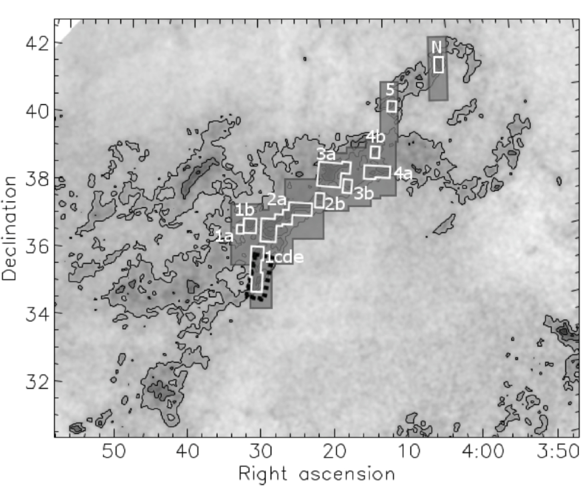
Figure 1: Integrated Spitzer mapped areas from the Gould Belt Survey and other projects. The grey boxed area shows the MIPS coverage; the white boxes show the IRAC coverage (with the sub-regions labelled); and the hatched black box shows the non-GBS survey data in the field from Gutermuth et al. (2009). These regions are schematic to give a general picture of the layout of the coverage and to identify the subregions. The greyscale is the extinction map of Dobashi et al. (2005). Contours show the $A_{V}$ levels of 1, 3 and 5 mag.

The areas mapped are shown in Figure 1. The MIPS coverage is more contiguous than the IRAC coverage due to the mapping modes of the two instruments. Observations were designed to cover regions with $\rm{A}_{V}$ $>3$ within the extinction maps of Dobashi et al. (2005). All areas were observed twice with IRAC and MIPS cameras with the AORs and dates of the observations compiled in Tables 1 and 2. The two epochs were compared to remove transient asteroids that are numerous at the low ecliptic latitude of these observations.

The GBS survey data and the LkH$\alpha$ 101 data from Gutermuth et al. (2009) were processed through the c2d pipeline. Details of the data processing are available in Evans et al. (2007). Briefly, the data processing starts with a check of the images whereupon image corrections are made for obvious problems. Mask files are created to remove problematic pixels. The individual frames are then mosaicked together, with one mosaic created for each epoch and one joint mosaic as well. Sources are detected in each mosaic and then re-extracted from the stack of individual images which include the source position. Finally, the source lists for each wavelength are band-merged, and sources not detected at some wavelengths are “band-filled” to find appropriate fluxes or upper limits at the positions which had clear detections at other wavelengths.

As noted by Harvey et al. (2008), the details of this data reduction are essentially the same as that of the original c2d datasets except that the input to the c2d pipeline are products of later versions of the Spitzer BCD pipeline. The c2d processing of IRAC data was described by Harvey et al. (2006), and the MIPS data processing was described by Young et al. (2005) and Rebull et al. (2007). Harvey et al. (2007) describe additional reduction processes which we have used for the AMC data.

3 Star-forming Objects in the AMC

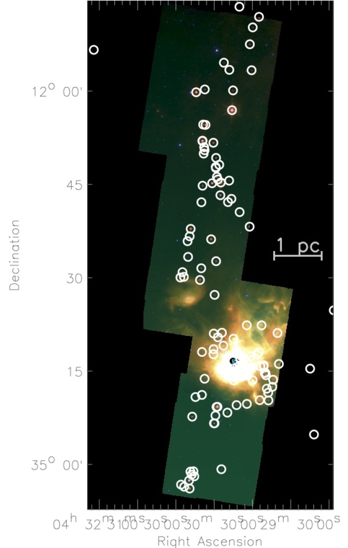
Figure 2: False colour image with 4.5 µm (blue), 8 µm (green), and 24 µm (red) of the IRAC 1cde fields with YSO positions are overlaid. (Similar figures for other IRAC regions are shown in Figures 3 – 5.)

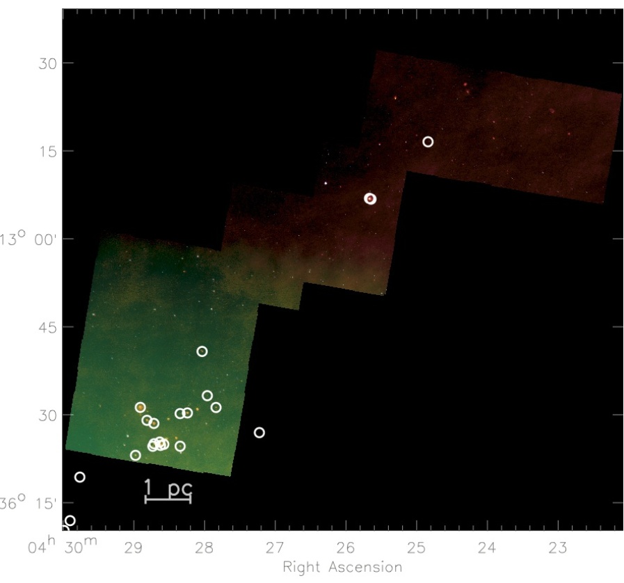
Figure 3: False colour image with 4.5 µm (blue), 8 µm (green), and 24 µm (red) of the IRAC 2a field with YSO positions are overlaid. (Similar figures for other IRAC regions are shown in Figures 2, 4, and 5.)

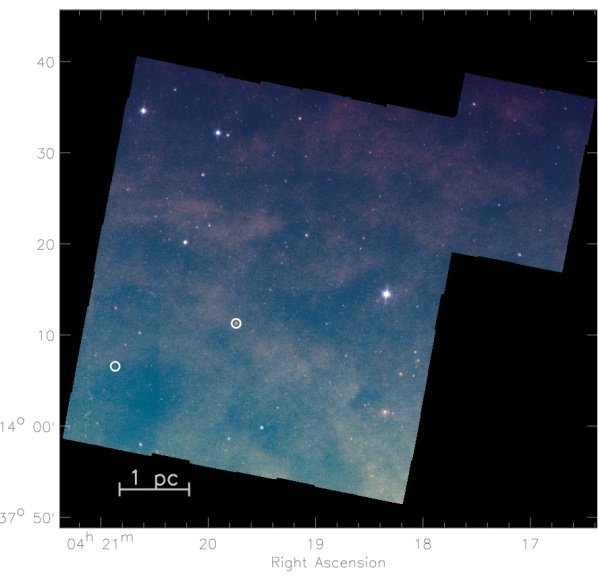
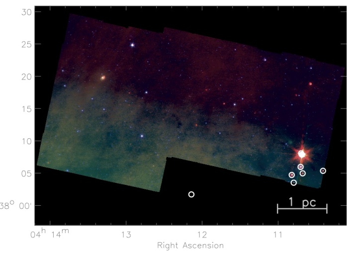
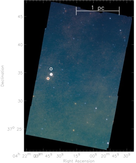
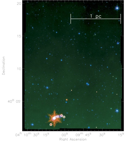
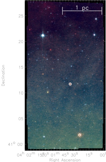
Figure 4: False colour image with 4.5 µm (blue), 8 µm (green), and 24 µm (red) of the IRAC fields 3a, 4a, 2b, 5, and North (left to right, top to bottom) with YSO positions are overlaid. These regions contain only a few YSOs each. (Similar figures for other IRAC regions are shown in Figures 2, 3, and 5.)

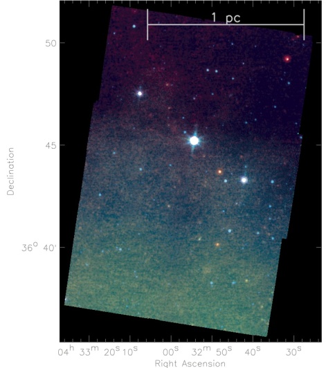
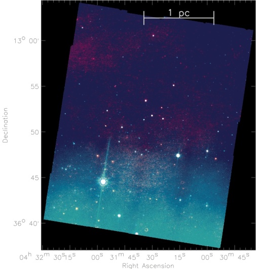
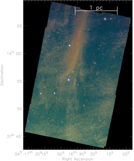
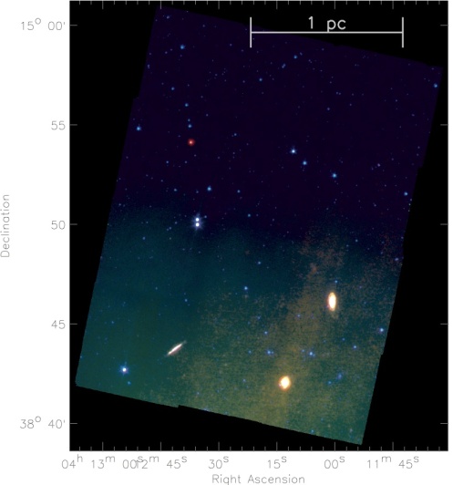
Figure 5: False colour image with 4.5 µm (blue), 8 µm (green), and 24 µm (red) of the IRAC fields 1a, 1b, 3b, and 4b (left to right, top to bottom) with YSO positions are overlaid. These regions do not contain YSOs. (Similar figures for other IRAC regions are shown in Figures 2 – 4.)

Figures 2 – 5 show RGB mosaics for the IRAC covered regions using 4.5 µm (blue), 8.0 µm (green) and 24 µm (red) data with the positions of YSOs overlaid. The diffuse 8.0 µm emission is strongly concentrated at the eastern edge of the cloud, near the well-known object LkH$\alpha$ 101. The LkH$\alpha$ 101 data are taken from and have been discussed by Gutermuth et al. (2009).

3.1 YSO Selection

The majority of objects in our fields are not YSOs. The maps are contaminated by background/foreground stars and background galaxies. We have selected our YSO candidates (YSOcs) by various methods, augmenting the list where possible based on data outside the Spitzer IRAC/MIPS wavelength bands. The fundamental criteria use IRAC, MIPS and 2MASS data (Cutri et al. 2003) and are based on identification of infrared excess and brightness limits below which the probability of detection of external galaxies becomes high. The total number of sources is 704,045. In regions observed by both IRAC and MIPS, the YSOc selection follows that of Harvey et al. (2008). We refer to these as IRAC+MIPS YSOcs. For objects with upper limits on the MIPS 24 µm flux, we follow the method outlined by Harvey et al. (2006). We refer to these as IRAC-only YSOcs. In regions observed only by MIPS and not IRAC, we have used the formalism of Rebull et al. (2007), except we use a tighter 2MASS K_S cut of [K_S] $<13.5$. This tighter magnitude cut removed objects that were similar in color and magnitude to others that had already been eliminated. We further remove galaxies from the MIPS-only source list by including photometry from the Wide-field Infrared Survey Explorer (WISE; Wright et al. 2010) and applying color cuts suggested by Koenig et al. (2012) (see their Figure 7) and requiring the WISE Band 2 magnitude criterion of [4.6] $<$ 12. We refer to these as MIPS-only YSOcs. Note that the MIPS-only YSOcs were not observed with IRAC, as opposed to the IRAC-only YSOcs which were observed, but not detected, with MIPS.

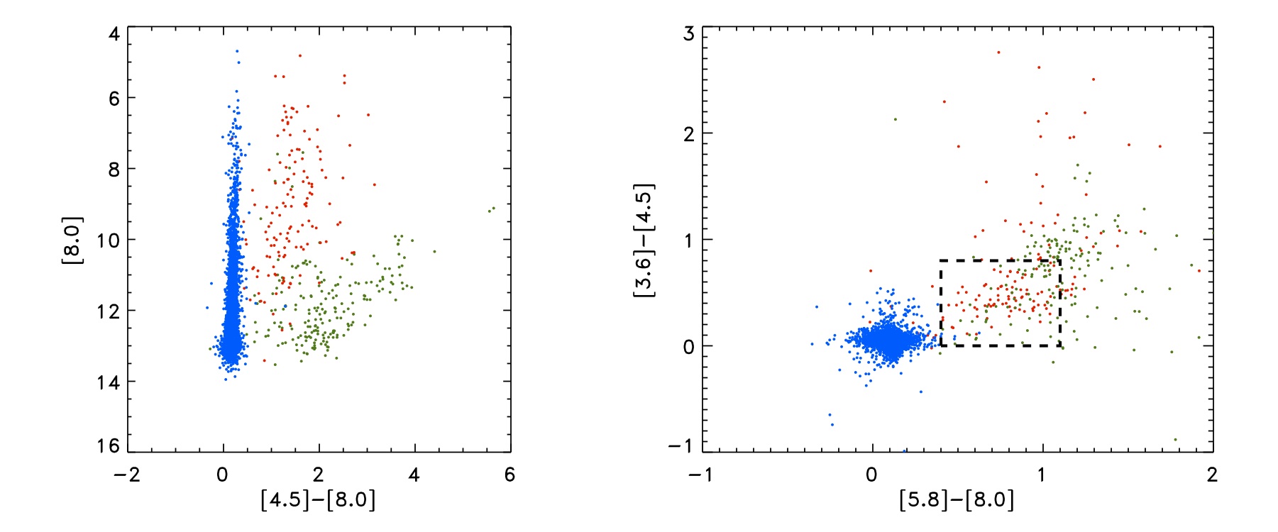
Figure 6: IRAC colors of the sources in the the regions observed with IRAC. Stars are in blue; YSOs are in red; and “other sources” (e.g., galaxies) are in green. The boxed region on the right panel marks the approximate domain of Class II sources identified by Allen et al. (2004).

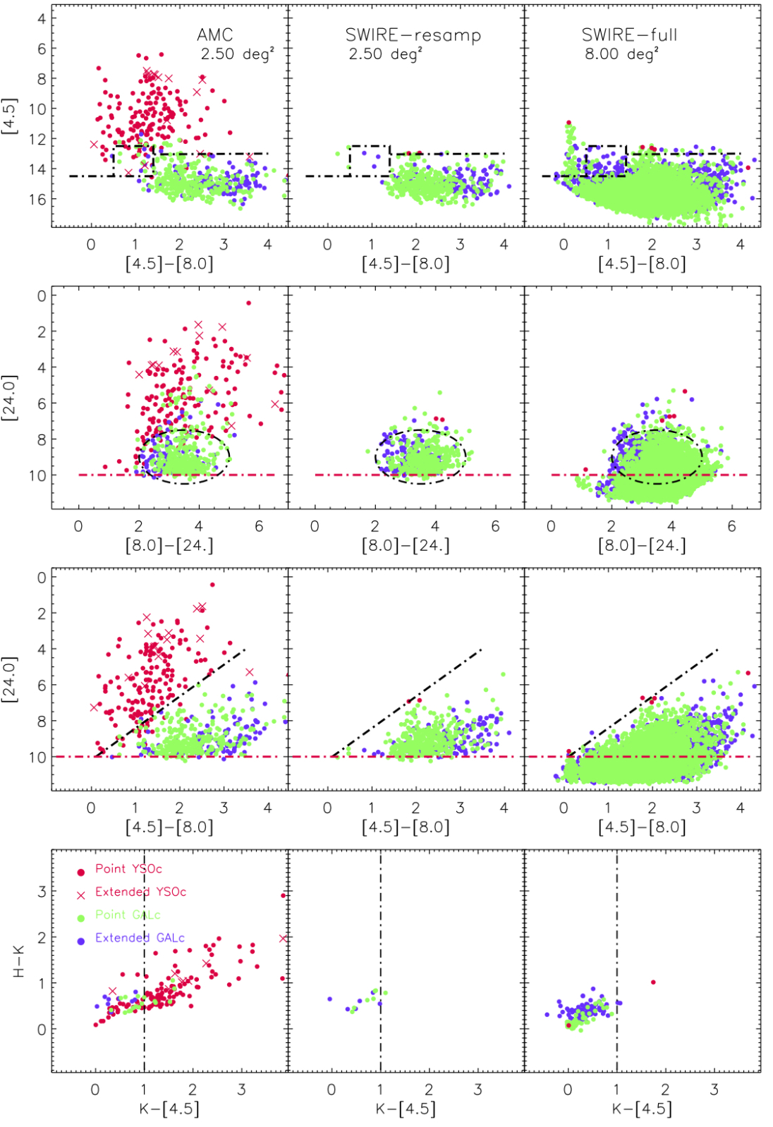
Figure 7: Color-magnitude and color-color diagrams for the AMC (left), the SWIRE dataset resampled to match our sensitivities and measured extinction (middle), and the full SWIRE dataset (right). The black dash-dot lines show soft boundaries for YSO candidates whereas the red dash-dot lines show hard limits, fainter than which objects are not included as YSO candidates.

Figure 6 shows the IRAC color-magnitude and color-color diagrams relevant for classifying IRAC-only sources. The different domains occupied by stars, YSOcs, and other (e.g., extragalactic) sources are are shown.

For sources in regions observed by both IRAC and MIPS, Figure 7 shows the color and magnitude boundaries used to remove sources that are likely extragalactic. This identification is done by comparing the observed fluxes and colors to results from the SWIRE extragalactic survey (Surace et al. 2004). The sources in the AMC field are compared to a control catalogue from the SWIRE dataset that is resampled to match our sensitivity limits and the extinction level derived for the AMC. (See Evans et al. 2007 for a complete description.)

Finally, we vetted the YSOcs through individual inspection of the Spitzer maps (and optical images where available), and determined that 24 of the original 159 IRAC+MIPS YSOcs, 14 of the original 17 IRAC-only YSOcs, and 56 (26 based on WISE and other photometric criteria) of the original 84 MIPS-only YSOcs were unlikely to be YSOs. Henceforth we refer to the list of vetted YSOcs, totalling 166, as YSOs to distinguish them from the raw unvetted list. While we have undergone an extensive process to construct a list of sources that are very likely to be YSOs, we stress that these YSOs have not been confirmed spectroscopically. Table 3 lists the final source counts for objects in the observed fields. The IRAC and MIPS fluxes of the IRAC+MIPS and IRAC-only YSOs are listed in Table 4. The 70 µm fluxes have been listed where available. (There are fewer YSOs with fluxes at 70 µm because of the lower sensitivity and, in some cases, the bright background.) The fluxes of MIPS-only vetted YSOs are listed in Table 5 with their WISE and MIPS fluxes (and IRAC fluxes where available). In Tables 4 and 5, we have noted which YSOs are in regions of low column density ($N_{\rm{H2}}<5\times 10^{21}$ cm^-2) according to the column density maps by Harvey et al. (2013), as these are more likely to be contaminants than YSOs in regions of high column density.

We compare our final YSO source list to those found for LkH$\alpha$ 101 in Gutermuth et al. (2009). All 103 YSOs in Gutermuth et al. (2009) are identified as sources in our catalogue with positions that are within a couple tenths of an arcsecond agreement. Where this work and Gutermuth et al. (2009) provide fluxes, they agree at the shorter IRAC bands (IRAC1-3) typically within 0.05 – 0.1 mag. At IRAC4 and MIPS1, the agreement is typically within 0.2 mag. These differences are what one might expect for PSF-fitting (used here) versus aperture fluxes (used by Gutermuth et al. 2009) at wavelengths where there is substantial diffuse emission. (Recall that we have incorporated their dataset into our own.) Therefore no previously identified sources have been missed in this study, and our measurements agree well with those of Gutermuth et al. (2009). Note, however, that the different classification methods used in this work and by Gutermuth et al. (2009) each yield a different total number of YSOs in this region; we have identified 42 YSOs whereas Gutermuth et al. (2009) identified 103. Our total breaks down into 7 YSOs identified here that were not identified by Gutermuth et al. (2009) and 35 YSOs shared between the two lists. (The c2d pipeline identified 47 YSOcs that were listed as YSOs by Gutermuth et al. (2009), but 12 were removed during the vetting process.) The major source of this discrepancy is that we require 4 (or 5) band photometry with S/N $\geq 3$ in IRAC (and MIPS 24 µm bands) to identify YSO candidates. Such criteria are especially difficult to satisfy in the region of bright and diffuse emission around LkH$\alpha$ 101. Therefore, our results do not contradict those in Gutermuth et al. (2009), rather we believe that the stringent criteria used here have excluded some YSOs. We keep these criteria for consistency with other c2d and Spitzer GBS observations and analyses, but note the limitations in such a bright region.

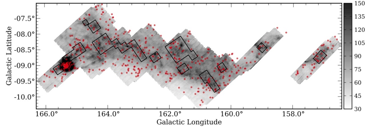
Figure 8: Sources with SEDs consistent with a reddened stellar photosphere and a dust component (IR excess) but for which detections with S/N $\geq 3$ across all 4 IRAC bands, required to considered a YSOc, did not exist (see text). The positions of these sources are plotted against the 160 µm greyscale (colorbar units are MJy sr^-1). The striking over-density at the center of LkH$\alpha$ 101 compared to other IRAC+MIPS regions (marked by black lines) suggests that we are missing veritable YSOs in this region. The robust set of measurements required to identify whether a source is a likely YSO or background galaxy is difficult to attain in this region of very bright emission.

The diffuse emission problem is isolated to the immediate vicinity of LkH$\alpha$ 101. To demonstrate this point, in Figure 8 we have plotted the location of all the sources having an SED consistent with being a reddened stellar photosphere and an associated dust component, which do not have S/N $\geq 3$ at all IRAC bands. The SEDs of these sources are classified as ‘star+dust’ in our catalogue. Of the 56 YSOs listed by Gutermuth et al. (2009) that were not identified as YSOs in this work, the majority of them (34 of 56) have a ‘star+dust’ SED. There is a total of 465 ‘star+dust’ sources without robust 4-band IRAC fluxes in the AMC field. These sources are relatively evenly distributed throughout the field, with the exception of a striking over-density at the center of LkH$\alpha$ 101 compared to other IRAC regions. Therefore, we believe this over-density is an effect of the difficulty in getting detections with S/N $\geq 3$ across 4 bands in the bright LkH$\alpha$ 101 region and not that there are significantly fewer YSOs than suggested by Gutermuth et al. (2009).

Harvey et al. (2013) identified 60 YSOs in the AMC with Herschel/PACS, 49 of which are also identified in this work. Four of these Spitzer-identified YSOs are members of pairs of YSOs that are blended in the Herschel images. Herschel is more sensitive to the rising- and flat-spectrum sources, i.e., of the other 45 Spitzer-identified YSOs that are also detected in the Herschel maps, most (76%) are Class I/F objects, and the remaining 24% are Class IIs.

3.2 YSO classification

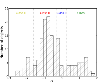
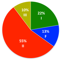
Figure 9: Left: Distribution of $\alpha$ values (the slope of the SED in the IR) used to determine the ‘class’ of the YSOs in the AMC. The vertical dotted lines mark the boundaries between the different classes as defined by Greene et al. (1994). Right: Pie chart for the AMC showing the percentage of sources in each SED class. Green is Class I; blue is Flat; red is Class II; and yellow is Class III (colors are the same as in Figure 18).

The YSOs are classified according to the slope of their SED in the infrared (see Evans et al. 2009 for a description). The spectral index, $\alpha$, is given by

$$\alpha\equiv{{d\log(\lambda S(\lambda))}\over{d\log(\lambda)}}$$ (1)

and determined by fitting the photometry between 2 µm and 24 µm. The distribution of $\alpha$ values is shown in Figure 9 along with the relative number of YSOs in each SED class. The majority of YSOs identified in the cloud are Class II objects (55%). The percentage of sources in each SED class for the AMC is strikingly similar to that of Perseus (23%, 11%, 58%, and 8% for Class Is, Fs, IIs and IIIs, respectively; Evans et al. 2009).

Table The Spitzer Survey of Interstellar Clouds in the Gould Belt. VI. The Auriga-California Molecular Cloud observed with IRAC and MIPS lists the breakdown of Class Is, Fs, and IIs for the AMC and other clouds in the GB and c2d surveys to estimate their relative ages. We did not include Class IIIs in this analysis since this population is typically incomplete in Spitzer surveys (e.g., see discussions in Harvey et al. 2008; Evans et al. 2009; Gutermuth et al. 2009) due to their weak IR excess. This simplifies the comparison to other clouds where the completeness limits may vary. We compared the ratio of Class Is and Fs to Class IIs, $N_{\rm{I+F}}$/$N_{\rm{II}}$, for the different cloud populations in other GB and c2d surveys which use the same classification scheme. We also include YSOs in the OMC identified with Spitzer by Megeath et al. (2012); since they use a different classification scheme however, we have re-calculated the $\alpha$ values for their sample. The Class I/F lifetime is relatively short compared to the Class II lifetime, and therefore a higher ratio indicates a younger population (see discussion in Evans et al. 2009). The high number of Class Is and Fs suggests that the AMC is relatively young compared to other clouds.

Finally, we also compared the number of YSOs per square degree in the AMC (11.5 deg²) to that in the OMC (14 deg²). The OMC is forming vastly larger amounts of stars. It has 237 YSOs per deg² whereas the AMC only has 13 YSOs per deg², a factor of about 20 fewer. Even if we only compare the number of YSOs in the OMC with 4 band photometry (as this was the source of the discrepancy between the total number of YSOs around LkH$\alpha$ 101 identified in this work and by Gutermuth et al. 2009, who use a similar identification method to Megeath et al. 2012), this still suggests that there is at least a factor 15 more YSOs in the OMC than in the AMC. Despite the differences in identification methods used for the OMC and for the AMC, it is clear that the OMC is forming far more stars than the AMC is. The YSOs in the OMC are also concentrated much more strongly than the AMC, despite both clouds having comparable sizes and masses. We note that Lada et al. (2009) attribute the difference between the amount of star formation to the different amounts of material at high $\rm{A}_{V}$/column density.

4 Spectral Energy Distribution Modeling

Optical data of the YSOs were downloaded from the USNO NOMAD catalogue (Zacharias et al. 2004). SEDs of the YSOs are shown in Figures 10 and 11 (Class Is and Class Fs), 12 – 14 (Class IIs) and 15 (Class IIIs). We were able to perform relatively detailed modelling of the stellar and dust components of the Class II and Class III sources (YSOs which are not heavily obscured by dust). The luminosities of sources in the earlier classes are presented in Dunham et al. (2013). The majority of the Class II and Class III sources are likely in the physical stage where the stellar source and circumstellar disk are no longer enshrouded by a circumstellar envelope. We note that the observed “class” does not always correspond to the associated physical stage of the YSO (see discussion in Evans et al. 2009) and that some Class IIs may be sources, viewed pole-on, with circumstellar envelopes that are only beginning to dissipate. Conversely, an edge-on disk without an envelope could look like a Class I object.

Our SED modelling methods follow those used by Harvey et al. (2007) (and similar works since, e.g., Merín et al. 2008, Kirk et al. 2009) to model the SEDs. The stellar spectrum of a K7 star was fit to the SEDs by normalizing it to the de-reddened fluxes in the shortest available IR band of J, K or IRAC1. We use the extinction law of Weingartner & Draine (2001) with $\rm{R}_{V}$$=5.5$ to calculate the de-reddened fluxes. The $\rm{A}_{V}$ value was estimated by matching the de-reddened fluxes with the stellar spectrum. In eight cases, we used an A0 spectrum when the K7 spectrum was unable to produce a reasonable fit. The use of only two stellar spectra is of course over-simplified; how-

Figure 10: SEDs of Class I and Flat sources. The YSO ID, from Tables 4 and 5, is shown in the upper right of each panel along with the Class (I or F) of the YSO.

Figure 11: continued from Figure 10.

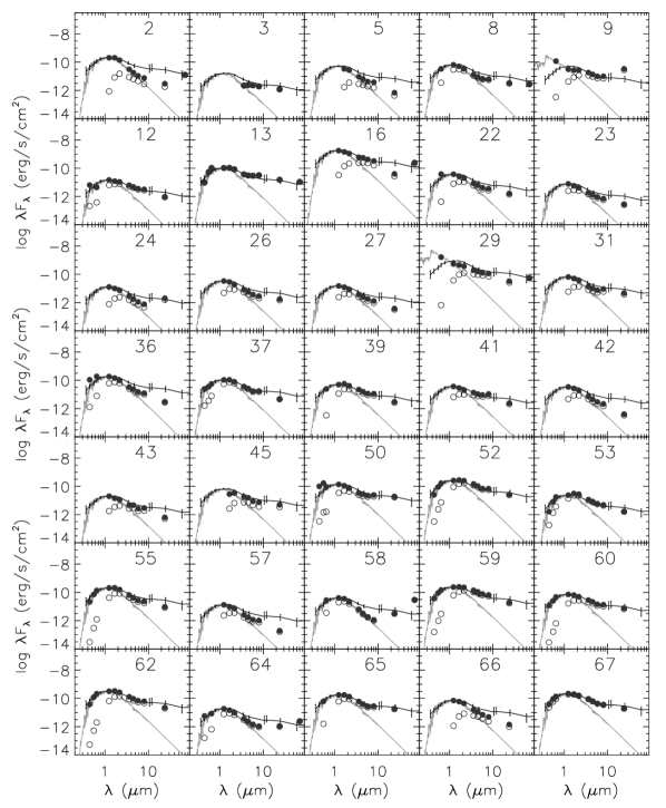
Figure 12: SEDs of Class II sources. The YSO ID, from Tables 4 and 5, is shown in the upper right of each panel. The observed fluxes are plotted with unfilled circles. The de-reddened fluxes are plotted with filled circles. The grey line plots the model stellar spectrum fit to the shorter wavelengths. The black line shows the median SED of T Tauri stars in Taurus (with error bars denoting quartiles of the distribution, D’Alessio et al. 1999) normalized to the B band flux and J band flux of the K7 and A0 stellar spectrum models, respectively.

Figure 13: continued from Figure 12.

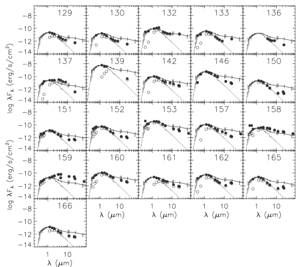
Figure 14: continued from Figure 12.

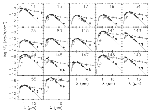
Figure 15: SEDs of Class III sources. The YSO ID, from Tables 4 and 5, is shown in the upper right of each panel. The observed fluxes are plotted with unfilled circles. The de-reddened fluxes are plotted with filled circles. The grey line plots the model stellar spectrum fit to the shorter wavelengths. The black line shows the median SED of T Tauri stars in Taurus (with error bars denoting quartiles of the distribution, D’Alessio et al. 1999) normalized to the B band flux and J band flux of the K7 and A0 stellar spectrum models, respectively.

ever, it produces adequate results for the purposes of this study. More exact spectral typing is difficult with only the photometric data presented here and the uncertainties in $\rm{A}_{V}$. We nevertheless obtain a broad overview of the disk population with the applied assumptions. Tables 7 and 8 list the stellar spectrum, the $\rm{A}_{V}$ value, and stellar luminosity ($L_{\rm{star}}$) used for the stellar models of each source’s SED for the Class II and Class III YSOs, respectively.

4.1 Second order SED parameters $\alpha_{\rm{excess}}$ and $\lambda_{\rm{turnoff}}$

The first order SED parameter $\alpha$ is used as a primary diagnostic of the excess and circumstellar environment and to separate the YSOs into different “classes” (§ 3.2). Once we have a model of the stellar source, however, we are able to characterize the circumstellar dust better. For each source we determined the values of $\alpha_{\rm{excess}}$ and $\lambda_{\rm{turnoff}}$ defined by Cieza et al. (2007) and Harvey et al. (2007) and used in many works since. $\lambda_{\rm{turnoff}}$ is the longest measured wavelength before an excess greater than 80% of the stellar model is observed. If no excess $>$ 80% is observed, than $\lambda_{\rm{turnoff}}$ is set to 24 µm. $\alpha_{\rm{excess}}$ is the slope of the SED at wavelengths longward of $\lambda_{\rm{turnoff}}$. $\alpha_{\rm{excess}}$ is not calculated for YSOs with $\lambda_{\rm{turnoff}}$ $=24$ µm  as there are not enough data points to determine the slope of the excess. These parameters provide a better characterization of the excess since $\alpha$ can include varying contributions from the stellar and dust components.

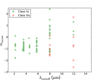
Figure 16: Distribution of $\alpha_{\rm{excess}}$ and $\lambda_{\rm{turnoff}}$ for Class II and Class III sources. The Class IIIs with $\lambda_{\rm{turnoff}}$$=24$ µm (IDs 15, 19, 80, and 148) are not shown as those sources typically do not have excess measured across a wide enough range to calculate reliable values of $\alpha_{\rm{excess}}$.

Figure 16 shows the distribution of $\alpha_{\rm{excess}}$ and $\lambda_{\rm{turnoff}}$ for the Class IIs and Class IIIs. Class II and Class III YSOs with long $\lambda_{\rm{turnoff}}$ and positive $\alpha_{\rm{excess}}$  (YSOs 2, 24, 58, 64, 74, 102, 108, 113, 115, and 133 in the 8 µm bin and YSOs 145, 150, 162, and 165 in the 12 µm bin of Figure 16) are good classical transition disk candidates; the lack of near-IR excess but large mid-IR excess is a sign of a deficit of material close to the star within a substantial disk. Cieza et al. (2012) have recently done a study on the transition disks in the AMC, Perseus and Taurus and identify six transition disk candidates in the AMC, three of which are also in our list of candidates (YSOs 58, 102 and 115). Of their remaining candidates, two were debris-like disks (YSOs 11 and 54) and the other was not identified in our YSO list. The larger distribution of $\alpha_{\rm{excess}}$ for sources with longer $\lambda_{\rm{turnoff}}$ is consistent with distributions found for other disk populations (e.g., Cieza et al. 2007; Alcalá et al. 2008; Harvey et al. 2008; Merín et al. 2008).

4.2 Disk luminosities

Figure 17 shows the ratio of the disk luminosities to stellar luminosities for the Class II and Class III sources. The disk luminosity is the integral of the observed excesses. (The excess at a given wavelength is calculated by subtracting the flux of the stellar model at that wavelength from the observed flux). The distribution of $L_{\rm{disk}}$$/$$L_{\rm{star}}$ for Class II and III sources in the AMC is similar to that found for other c2d and GB surveys with Spitzer (Serpens: Harvey et al. 2007, IC 5146: Harvey et al. 2008, Chameleon II: Alcalá et al. 2008, Lupus: Merín et al. 2008, and the Cepheus Flare: Kirk et al. 2009). We find the Class III sources in the regions typically occupied by sources with passive disks and debris disks (e.g., 0.02 $<$ $L_{\rm{disk}}$$/$$L_{\rm{star}}$$<$ 0.08 for passive disks; Kenyon & Hartmann 1987). The low disk luminosity may be attributable to the lack of mid-IR excess at IRAC wavelengths in these sources’ SEDs.

Figure 17: The ratio of the disk luminosity to the stellar luminosity for Class II and Class III sources. Also shown are the typical boundaries found for accreting disks, passive disks and debris disks (Kenyon & Hartmann 1987).

4.3 Questionable Class III sources

It is possible that some of the Class III sources identified here are field giants. Oliveira et al. (2009) followed up on 150 Spitzer identified YSOs in Serpens and obtained 78 optical spectra with sufficient signal-to-noise. They showed that there were at least 20 giant contaminants in this list, 18 of which were identified as Class III sources. The more scattered spatial distribution of Class IIIs throughout the AMC is consistent with this idea that they are contaminants. Additionally, five of our Class III objects (YSOs 11, 141, 144, 148, 164) have very high luminosities ($>100$ L_⊙). Four of these objects (YSOs 141, 144, 148, 164), as well as YSO 149 which is not of particularly high luminosity, are quite removed from the areas of high extinction towards the AMC (see Figure 18 in the following section) and regions of low column density ($N_{\rm{H2}}<5\times 10^{21}$ cm^-2, see § 3.1).

5 Spatial Distribution of Star Formation

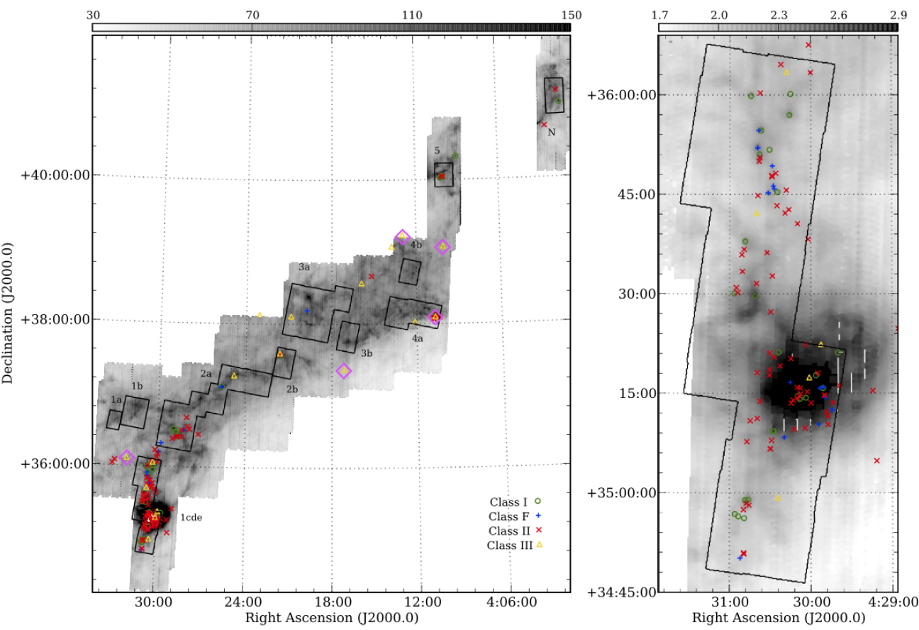
Figure 18: Left: The positions of YSOs and IRAC fields in Auriga. The greyscale is the MIPS 160 $\mu$m map (colorbar units are MJy sr^-1) and the YSOs are marked according to their classification: green circles denote Class Is; blue $+$s denote Class Fs; red $\times$s denote Class IIs; yellow triangles denote Class IIIs. The magenta diamonds mark the Class III sources of high luminosities that are likely contaminants (see § 4.3). IRAC fields are outlined in black and labelled. (Note that some YSOs fall beyond the 160 µm coverage because it is slightly offset from the 24 µm coverage that is used for YSO identification.) Right: Close-up of the region around LkH$\alpha$ 101. The greyscale is the log (base 10) of the flux (colorbar units are $\log$(MJy sr^-1)). The centre of the field is entirely saturated. As is evident, there are some YSOs outside the IRAC coverage area. This list of MIPS-only YSOs has been trimmed by using WISE data to remove more objects that are likely background galaxies.

The spatial distribution of IRAC/MIPS-identified YSOs by class is shown in Figure 18. A close-up of the region surrounding the LkH$\alpha$ 101 cluster and the cluster extension along the filament is also included so the relatively densely clustered YSOs can be better distinguished. Figure 18 shows that the bulk of star formation in the AMC has been concentrated in this southern region of the cloud; the majority of the identified YSOs (79%) are in this area. (Note that the number of YSOs in that region is a lower limit as it is likely that a significant number of YSOs in the LkH$\alpha$ 101 region are not identified, see discussion at the end of $\S$ 3.1.)

5.1 Identification of YSO groups

We performed a clustering analysis on the identified Class I, F, and II sources in the AMC to identify the densest regions of YSOs and the largest groups. The details of the analysis are described in Masiunas et al. (2012). We omit the Class III sources from the analysis to avoid the risk of including field giants (see for example § 4.3). We performed a minimum spanning tree (MST) analysis to identify groups of YSOs within the region. This analysis connects YSOs by the minimum distance to the next YSO to form a “branch” (Cartwright & Whitworth 2004). Figure 19 shows the cumulative distribution function (CDF) of the branch lengths between YSOs. This is used to determine the MST critical branch length, $\rm{L}_{\rm{crit}}$, that defines the transition between the branch lengths in the denser regions to the branch lengths in the sparser regions (Gutermuth et al. 2009). Therefore $\rm{L}_{\rm{crit}}$ is based on relative over densities of objects. We measure an $\rm{L}_{\rm{crit}}$ of 210″ for the AMC. Group memberships are defined by members which are all connected by branches of lengths less than $\rm{L}_{\rm{crit}}$. The boundary of a group is defined where the branch length between adjacent sources exceeds $\rm{L}_{\rm{crit}}$. Figure 20 shows that we have extracted four groups with 10 or more members (marked by colored convex hulls) and three groups with 5–9 members (marked with magenta circles). Table 9 lists the properties of these groups. The position of the group is given by its geometric center. The group’s effective radius, $R_{\rm{eff}}$, defines the radius of a circle with the same area as the convex hull containing the group members. The maximum radial distance to a member from the median position gives $R_{\rm{circ}}$, therefore a circle with this radius would contain all group members. Finally, the elongation of the group is determined by comparing $R_{\rm{circ}}$ to $R_{\rm{eff}}$ and represented by the aspect ratio, $R_{\rm{circ}}$${}^{2}/$$R_{\rm{eff}}$². The MST analysis on the full cloud recovers the clustering surrounding LkH$\alpha$ 101. The cluster subtends a larger area than that measured in Gutermuth et al. (2009) confirming their claim that there was star formation extended beyond their field of view. The star formation is mostly extended along the North-South direction of the cluster and therefore we measure a more elongated group than measured by Gutermuth et al. (2009). This is still the largest group in the AMC in terms of area and the number of members.

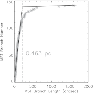
Figure 19: Cumulative distribution function (CDF) of MST branch lengths (asterisks). The solid lines represent linear fits to each end of the CDF. The dot-dash line marks $\rm{L}_{\rm{crit}}$ where the solid lines meet. The solid lines follow the CDF in the dense regions (steep line) and the sparser regions (shallow line).

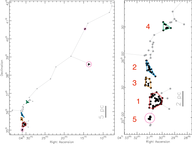
Figure 20: We extract four groups with 10 or more members (colored convex hulls) and three groups with 5–9 members (magenta circles) using an MST analysis. The right hand panel shows the enlarged southern region of the cloud where most of the groups are located. The red numbers adjacent to the groups correspond to the group number listed in Table 9.

As discussed in $\S$ 3.1, our analysis is likely to have underestimated the number of YSOs in the region around LkH$\alpha$ 101. To check the consistency of our analysis with Gutermuth et al. (2009), we ran the MST analysis on both YSO lists within the Gutermuth et al. (2009) area of 4-channel IRAC coverage. This leaves us with 41 of the YSOs presented here and 102 of those presented in Gutermuth et al. (2009). (There is one bright YSO in Gutermuth et al. 2009 that lies just outside their 4-channel IRAC coverage to the south. It was only observed at IRAC1 and IRAC3.) We get an $\rm{L}_{\rm{crit}}$ of 120″ for our cropped list of YSOs and an $\rm{L}_{\rm{crit}}$ of 73″ for the cropped Gutermuth et al. (2009) YSO list. (Note that running the analysis on the cropped field, which is dense compared to the rest of the cloud, yields a smaller $\rm{L}_{\rm{crit}}$ than when the analysis is run on the whole cloud. This is expected as $\rm{L}_{\rm{crit}}$ is based on over densities, as discussed above.) The ratio of the $\rm{L}_{\rm{crit}}$ values for the two YSO lists ($73/120=0.61$) agrees with our expectation that it should scale with the square-root of the density, and hence the cropped YSO count ($\sqrt{102/41}=0.63$). Therefore we report that the derived properties are consistent with those measured by Gutermuth et al. (2009). (Differences are expected as shown by Gutermuth et al. (2009) with their comparisons among several shared regions.) However, the missing YSOs at the centre of the cluster complicate any further comparison their results.

5.2 Comparison of grouped and non-grouped YSOs

We find 76% (113 of the 149) of the Class Is, Class Fs, and Class IIs are found in groups. Rather than compare the class fractions, given by $N_{\rm{I+F}}$/$N_{\rm{II}}$ in Table 9, we directly compare the underlying distribution of $\alpha$ to determine whether the distribution of YSOs within groups is consistent with the whole cloud. We get the same result for each group: a KS test on the $\alpha$ distribution of the group and the $\alpha$ distribution of the whole cloud shows that we cannot reject the hypothesis that they are drawn from the same sample (p-values $>$ 0.13). (We also did a KS test for each group with the extended population and found the same result.)

Similarly, we compared the properties of disks within groups and those not in groups by performing a KS test on the distributions of disk luminosities (p-value of 0.08), $\alpha_{\rm{excess}}$ (p-value of 0.9), and $\lambda_{\rm{turnoff}}$ (p-value of 0.9) and find no evidence that the two populations are drawn from different parent populations.

6 Summary

We observed the AMC with IRAC and MIPS aboard the Spitzer Space Telescope and identify 138 YSOs in the cloud. As our IRAC coverage is segmented, we complemented our more contiguous MIPS coverage with WISE data to further eliminate galaxies from the sample, leaving 28 MIPS-only YSOs remaining, bringing the total number of YSOs in the AMC to 166. We classified the YSOs based on the spectral slope of their SEDs between 2 µm and 24 µm and find 37 Class I objects, 21 Class F objects (flat spectrum sources), 91 Class II objects, and 17 Class III objects. The high fraction of Class Is and Class Fs suggests that the AMC is relatively unevolved compared to other star-forming clouds. Despite the similarity in cloud properties between the AMC and the OMC, there is a distinct difference in the star formation properties. The star formation in the AMC is also concentrated along its filament, however, it is also forming a factor of about 20 fewer stars than the OMC. Lada et al. (2009) find that there is much less material at high density in the AMC than in the OMC and attribute the difference in star formation to this. Further studies of the star formation and YSO population in the AMC are needed to highlight the differences of the two clouds given their similar age.

We modelled the SEDs of the Class II and Class III sources and their excesses by first fitting a K7 stellar spectrum to the optical and near-IR fluxes. The spectrum is normalized to the 2MASS flux (or the IRAC1 flux when 2MASS is unavailable) and we use an $\rm{A}_{V}$ value to match the spectrum of the stellar model to the de-reddened observed optical fluxes. An A0 stellar spectrum is used in the eight cases where a K7 spectrum is unable to provide a reasonable fit. Fitting a stellar spectrum allows us to measure the disk luminosities and characterize the excess. The excesses of the Class II and Class III sources were further parameterized by $\lambda_{\rm{turnoff}}$, the longest wavelength before an excess greater that 80% is measured, and $\alpha_{\rm{excess}}$, the slope of the SED at wavelengths longward of $\lambda_{\rm{turnoff}}$. $\lambda_{\rm{turnoff}}$ is a useful tracer for the proximity of dust to the star and consequently we identify fourteen classical transition disk candidates.

The bulk of the star formation in the AMC is in the southern region of the cloud. We included a clustering analysis to quantify the densest areas of star formation and to identify groups within the cloud. We find four groups with 10 or more members all in the region around LkH$\alpha$ 101 and its adjoining filament. We find three smaller groups with 5 – 9 members scattered throughout the cloud. The largest group is that around LkH$\alpha$ 101 and contains 49 members. We note that there are likely even more YSOs in this group since our YSO identification criteria of S/N $\geq 3$ in IRAC1-4 and MIPS1 are difficult to attain in this bright region.

Table 1: Summary of IRAC Observations

IRAC Sub-region	Size	AOR Sub-region ID	AOR Key (1st epoch, 2nd epoch)
	(sq. deg.)
AUR_1a	0.3 $\times$ 0.2	auri_irac6b	19972096, 19971584
AUR_1b	0.4 $\times$ 0.3	auri_irac6	20014336, 20014080
AUR_1c	0.9 $\times$ 0.3	auri_irac7	19980544, 19980288
		auri_irac7b	19984384, 19984128
AUR_1d	0.3 $\times$ 0.2	non-GB data	03654144
AUR_1e	0.3 $\times$ 0.3	auri_irac8	20013312, 20013056
AUR_2a	1.3 $\times$ 1.4	auri_irac3	19983360, 19983104
		auri_irac4	20016640, 20016384
		auri_irac5	19981824, 19981568
		auri_irac5b	19956480, 19956224
AUR_2b	0.4 $\times$ 0.3	auri_irac2	20018432, 20017920
AUR_3a	0.8 $\times$ 0.9	auri_irac1	19984640, 19967744
		auri_irac9	19978240, 19977984
AUR_3b	0.4 $\times$ 0.3	auri_irac9b	20012288, 20011776
		auri_irac9c	19976960, 19976192
AUR_4a	0.4 $\times$ 0.7	auri_irac10	19993344, 19993088
		auri_irac10b	19988992, 19988736
AUR_4b	0.3 $\times$ 0.3	auri_irac11	19961088, 19960832
AUR_5	0.3 $\times$ 0.3	auri_irac12	19992576, 19992064
AUR_NORTH	0.5 $\times$ 0.3	auri_irac13	19960320, 19959808

Table 2: Summary of MIPS Observations

MIPS Sub-region	Size	AOR Key
	(sq. deg)
AUR_1	1.2 $\times$ 3.2	20019712,19983872,20019456,19983616
AUR_2	1.6 $\times$ 2.6	20017152,19982336,20016896,19982080
AUR_3	1.0 $\times$ 2.0	20015360,20014848
AUR_4	1.4 $\times$ 2.2	19981312,19979520,19981056,19979008
AUR_5	0.5 $\times$ 1.9	20013824,20013568
AUR_NORTH	0.5 $\times$ 1.9	20011520

Table 3: Sources in the AMC Field

Sources	Number
Total	704045
YSO	166
Galc	322
Stellar	32579
2MASS	87745
Zero	247257
Something else	335976

Table 4: YSOs in the AMC Based on IRAC and MIPS

				3.6 µm	4.5 µm	5.8 µm	8.0 µm	24.0 µm	70.0 µm
ID	Name	Class	$\alpha$	(mJy)	(mJy)	(mJy)	(mJy)	(mJy)	(mJy)
1	04012455$+$4101490	I	2.04	0.50$\pm$0.03	4.06$\pm$0.20	7.94$\pm$0.38	8.49$\pm$0.41	352$\pm$ 32	8410$\pm$ 965
2	04013436$+$4111430	II	-1.00	10.5$\pm$ 0.5	9.66$\pm$0.46	8.99$\pm$0.44	7.65$\pm$0.36	14.7$\pm$ 1.4	288$\pm$ 30
3	04100064$+$4002361	II	-0.31	2.64$\pm$0.13	3.63$\pm$0.18	4.50$\pm$0.22	5.16$\pm$0.25	9.66$\pm$0.93	$\cdots$
4	04100263$+$4002482	I	0.98	0.60$\pm$0.04	0.99$\pm$0.05	0.96$\pm$0.06	0.91$\pm$0.06	49.3$\pm$ 4.6	$\cdots$
5	04100562$+$4002386	II	-0.79	3.46$\pm$0.20	3.65$\pm$0.20	3.74$\pm$0.20	4.18$\pm$0.20	3.51$\pm$0.68	$\cdots$
6	04100841$+$4002244	I	1.70	18.6$\pm$ 2.8	53.3$\pm$ 3.0	119$\pm$ 6	237$\pm$ 11	4770$\pm$ 470	24600$\pm$ 3550
7	04101116$+$4001262	I	1.99	0.066$\pm$0.006	0.35$\pm$0.02	0.34$\pm$0.03	0.27$\pm$0.04	41.1$\pm$ 3.8	$\cdots$
8	04104051$+$3805004	II	-0.78	12.9$\pm$ 0.6	11.5$\pm$ 0.5	11.6$\pm$ 0.6	14.9$\pm$ 0.7	25.1$\pm$ 2.3	64.0$\pm$13.1
9	04104163$+$3808058	II	-0.32	13.9$\pm$ 0.7	14.1$\pm$ 0.9	14.3$\pm$ 1.0	18.9$\pm$ 1.6	226$\pm$ 75	$\cdots$
10	04104109$+$3807545	I	2.03	1280$\pm$ 78	2150$\pm$ 132	4330$\pm$ 244	5530$\pm$ 304	11000$\pm$ 2200	$\cdots$
11	04104211$+$3805599	III	-2.26	341$\pm$ 25	210$\pm$ 12	151$\pm$ 9	87.1$\pm$ 4.4	43.9$\pm$ 4.2	$\cdots$
12	04104761$+$3803338	II	-0.87	6.21$\pm$0.32	6.14$\pm$0.33	6.11$\pm$0.30	7.42$\pm$0.37	7.18$\pm$0.70	$\cdots$
13	04104916$+$3804458	II	-0.49	44.1$\pm$ 2.2	46.3$\pm$ 2.2	57.0$\pm$ 2.7	85.0$\pm$ 4.1	123$\pm$ 11	253$\pm$ 26
14	04194467$+$3811219	F	-0.07	4.54$\pm$0.23	5.62$\pm$0.27	7.26$\pm$0.36	10.2$\pm$ 0.5	22.5$\pm$ 2.1	$\cdots$
15	04205246$+$3806358	III	-2.42	14.5$\pm$ 0.7	10.1$\pm$ 0.5	7.13$\pm$0.35	4.33$\pm$0.23	1.08$\pm$0.17	$\cdots$
16	04213795$+$3734418	II	-0.85	284$\pm$ 14	387$\pm$ 20	443$\pm$ 21	432$\pm$ 20	223$\pm$ 20	5530$\pm$ 1230
17	04213808$+$3735409	III	-1.64	1.88$\pm$0.09	1.71$\pm$0.08	1.29$\pm$0.07	0.77$\pm$0.06	0.92$\pm$0.20	$\cdots$
18	04214080$+$3733590	I	1.99	1.12$\pm$0.06	4.07$\pm$0.20	10.2$\pm$ 0.5	26.1$\pm$ 1.2	241$\pm$ 22	945$\pm$ 112
19	04244934$+$3716464	III	-2.27	6.19$\pm$0.30	4.14$\pm$0.20	3.05$\pm$0.16	1.89$\pm$0.11	0.91$\pm$0.20	$\cdots$
20	04253848$+$3707012	I	1.43	0.60$\pm$0.03	1.04$\pm$0.08	1.95$\pm$0.13	4.50$\pm$0.25	59.1$\pm$ 5.5	1350$\pm$ 152
21	04253979$+$3707082	F	-0.01	254$\pm$ 12	485$\pm$ 25	671$\pm$ 33	744$\pm$ 39	727$\pm$ 68	1160$\pm$ 157
22	04275080$+$3631264	II	-0.86	7.15$\pm$0.35	6.93$\pm$0.34	6.45$\pm$0.32	7.28$\pm$0.35	11.4$\pm$ 1.1	$\cdots$
23	04275826$+$3633265	II	-1.03	1.72$\pm$0.08	1.59$\pm$0.08	1.52$\pm$0.08	1.54$\pm$0.09	2.08$\pm$0.30	$\cdots$
24	04280289$+$3640586	II	-0.37	1.81$\pm$0.09	1.59$\pm$0.08	1.39$\pm$0.08	1.23$\pm$0.08	12.5$\pm$ 1.2	$\cdots$
25	04281515$+$3630286	F	0.25	7.28$\pm$0.36	10.4$\pm$ 0.5	13.8$\pm$ 0.7	18.3$\pm$ 0.9	61.3$\pm$ 5.7	75.4$\pm$13.8
26	04282116$+$3624478	II	-0.83	6.30$\pm$0.31	5.79$\pm$0.28	5.20$\pm$0.26	5.40$\pm$0.26	11.8$\pm$ 1.1	$\cdots$
27	04282136$+$3630215	II	-1.09	2.93$\pm$0.14	2.60$\pm$0.13	2.63$\pm$0.14	2.50$\pm$0.13	2.55$\pm$0.30	$\cdots$
28	04283509$+$3625064	I	0.88	10.7$\pm$ 0.5	27.5$\pm$ 1.3	45.8$\pm$ 2.2	62.1$\pm$ 2.9	237$\pm$ 21	840$\pm$ 92
29	04283789$+$3624553	II	-0.63	124$\pm$ 6	140$\pm$ 6	161$\pm$ 8	188$\pm$ 9	204$\pm$ 18	1240$\pm$ 123
30	04283856$+$3625289	I	1.14	0.83$\pm$0.04	1.56$\pm$0.08	1.56$\pm$0.09	1.99$\pm$0.11	143$\pm$ 13	896$\pm$ 96
31	04284335$+$3625117	II	-0.44	9.32$\pm$0.45	9.36$\pm$0.45	9.92$\pm$0.48	15.7$\pm$ 0.7	30.1$\pm$ 2.8	$\cdots$
32	04284367$+$3628393	I	1.16	1.34$\pm$0.07	3.58$\pm$0.18	4.01$\pm$0.19	4.01$\pm$0.20	192$\pm$ 17	2170$\pm$ 244
33	04284443$+$3624456	F	0.12	1.73$\pm$0.08	2.55$\pm$0.12	3.46$\pm$0.17	5.78$\pm$0.28	10.4$\pm$ 1.0	$\cdots$
34	04284958$+$3629107	I	0.47	3.08$\pm$0.15	5.70$\pm$0.27	7.60$\pm$0.37	9.14$\pm$0.44	51.0$\pm$ 4.7	93.2$\pm$16.9
35	04285530$+$3631225	I	1.18	17.9$\pm$ 0.9	51.0$\pm$ 2.4	83.1$\pm$ 4.0	109$\pm$ 5	752$\pm$ 70	4290$\pm$ 476
36	04285911$+$3623112	II	-1.23	30.7$\pm$ 1.5	28.5$\pm$ 1.4	24.9$\pm$ 1.2	27.2$\pm$ 1.3	21.9$\pm$ 2.0	$\cdots$
37	04293901$+$3516105	II	-1.00	37.0$\pm$ 2.1	35.0$\pm$ 1.8	29.5$\pm$ 1.6	41.0$\pm$ 2.1	36.8$\pm$ 3.5	$\cdots$
38	04294001$+$3521089	I	0.51	22.7$\pm$ 1.1	28.1$\pm$ 1.4	50.6$\pm$ 2.5	160$\pm$ 8	147$\pm$ 14	$\cdots$
39	04294358$+$3513386	II	-0.86	18.8$\pm$ 0.9	17.9$\pm$ 0.9	17.8$\pm$ 0.9	23.0$\pm$ 1.1	21.0$\pm$ 2.1	$\cdots$
40	04294421$+$3512300	F	-0.21	8.89$\pm$0.43	9.39$\pm$0.46	10.2$\pm$ 0.5	16.2$\pm$ 0.8	44.2$\pm$ 4.1	$\cdots$
41	04294728$+$3510192	II	-0.54	10.9$\pm$ 0.5	11.4$\pm$ 0.5	13.6$\pm$ 0.7	21.1$\pm$ 1.0	16.6$\pm$ 1.6	$\cdots$
42	04294742$+$3511335	II	-1.37	5.59$\pm$0.27	4.66$\pm$0.22	4.19$\pm$0.22	3.99$\pm$0.20	2.70$\pm$0.36	$\cdots$
43	04294854$+$3512125	II	-0.75	3.21$\pm$0.15	4.47$\pm$0.22	3.54$\pm$0.18	5.09$\pm$0.25	4.13$\pm$0.50	$\cdots$
44	04294921$+$3514227	F	-0.24	62.6$\pm$ 3.2	74.9$\pm$ 3.7	76.9$\pm$ 3.7	94.9$\pm$ 4.7	196$\pm$ 18	$\cdots$
45	04294961$+$3514438	II	-0.51	8.80$\pm$0.44	11.0$\pm$ 0.5	9.26$\pm$0.46	9.66$\pm$0.48	27.6$\pm$ 2.8	$\cdots$
46	04295084$+$3515579	F	-0.11	33.3$\pm$ 1.7	43.1$\pm$ 2.2	45.1$\pm$ 2.2	65.0$\pm$ 3.1	177$\pm$ 17	$\cdots$
47	04295101$+$3515475	I	0.74	5.80$\pm$0.30	8.90$\pm$0.44	15.3$\pm$ 0.8	31.1$\pm$ 1.5	98.6$\pm$11.0	$\cdots$
48	04295346$+$3515485	F	-0.26	17.7$\pm$ 0.9	17.9$\pm$ 0.9	21.0$\pm$ 1.1	31.5$\pm$ 1.9	79.0$\pm$ 8.4	$\cdots$
49	04295415$+$3510216	F	0.08	2.44$\pm$0.12	4.56$\pm$0.22	6.10$\pm$0.32	8.85$\pm$0.44	16.5$\pm$ 1.6	$\cdots$
50	04295479$+$3518025	II	-0.32	29.6$\pm$ 1.5	32.0$\pm$ 1.6	35.0$\pm$ 1.8	51.2$\pm$ 3.4	135$\pm$ 12	$\cdots$
51	04295627$+$3517429	I	0.61	10.0$\pm$ 0.5	17.4$\pm$ 0.9	23.1$\pm$ 1.3	28.3$\pm$ 2.6	57.7$\pm$11.2	$\cdots$
52	04295976$+$3513342	II	-0.81	139$\pm$ 8	128$\pm$ 6	114$\pm$ 5	151$\pm$ 8	195$\pm$ 18	$\cdots$
53	04300016$+$3603227	II	-1.05	12.2$\pm$ 0.6	11.4$\pm$ 0.5	10.6$\pm$ 0.5	11.8$\pm$ 0.6	12.9$\pm$ 1.2	$\cdots$
54	04300114$+$3517246	III	-1.93	75.7$\pm$ 4.0	48.0$\pm$ 2.5	30.8$\pm$ 1.6	22.9$\pm$ 1.5	26.5$\pm$ 3.4	$\cdots$
55	04300263$+$3515143	II	-1.00	53.3$\pm$ 2.7	44.5$\pm$ 2.2	41.0$\pm$ 2.1	46.4$\pm$ 2.7	66.4$\pm$ 7.3	$\cdots$
56	04300363$+$3514201	I	0.75	8.19$\pm$0.57	12.5$\pm$ 0.6	17.6$\pm$ 1.3	31.4$\pm$ 4.1	37.4$\pm$11.2	$\cdots$
57	04300423$+$3509459	II	-1.17	2.06$\pm$0.10	1.85$\pm$0.09	1.73$\pm$0.10	2.02$\pm$0.12	1.33$\pm$0.26	$\cdots$
58	04300425$+$3522238	II	-0.62	6.47$\pm$0.37	4.25$\pm$0.21	3.23$\pm$0.25	2.69$\pm$0.60	24.8$\pm$ 2.5	688$\pm$ 118
59	04300743$+$3514579	II	-0.88	124$\pm$ 6	127$\pm$ 6	121$\pm$ 5	139$\pm$ 7	137$\pm$ 13	$\cdots$
60	04300773$+$3515484	II	-0.77	24.3$\pm$ 1.2	24.6$\pm$ 1.2	22.2$\pm$ 1.3	27.6$\pm$ 2.0	53.8$\pm$12.8	$\cdots$
61	04300825$+$3514100	I	0.46	9.62$\pm$0.48	14.9$\pm$ 0.7	19.3$\pm$ 1.1	27.1$\pm$ 2.0	119$\pm$ 13	$\cdots$
62	04300874$+$3514375	II	-0.84	107$\pm$ 5	105$\pm$ 5	105$\pm$ 5	127$\pm$ 8	158$\pm$ 38	$\cdots$
63	04300951$+$3514403	I	0.81	8.53$\pm$0.51	12.5$\pm$ 0.6	16.6$\pm$ 1.6	24.6$\pm$ 5.2	334$\pm$ 33	$\cdots$
64	04300980$+$3540355	II	-0.89	3.61$\pm$0.18	2.96$\pm$0.14	2.46$\pm$0.13	2.47$\pm$0.13	8.30$\pm$0.79	57.0$\pm$ 9.0
65	04300991$+$3515539	II	-0.94	56.8$\pm$ 3.2	48.4$\pm$ 2.9	44.8$\pm$ 2.8	63.2$\pm$ 4.0	139$\pm$ 42	$\cdots$
66	04301234$+$3509346	II	-0.99	7.18$\pm$0.35	7.73$\pm$0.37	7.17$\pm$0.35	6.30$\pm$0.30	7.86$\pm$0.76	$\cdots$
67	04301309$+$3513586	II	-0.90	107$\pm$ 7	93.5$\pm$ 4.8	81.6$\pm$ 4.6	93.2$\pm$ 7.1	153$\pm$ 15	$\cdots$
68	04301453$+$3513326	II	-0.39	81.4$\pm$ 7.7	96.1$\pm$ 4.9	96.3$\pm$ 5.0	108$\pm$ 7	160$\pm$ 27	$\cdots$
69	04301474$+$3520143	II	-0.60	136$\pm$ 10	146$\pm$ 8	166$\pm$ 8	191$\pm$ 11	197$\pm$ 19	$\cdots$
70	04301495$+$3600085	I	1.77	0.22$\pm$0.01	1.07$\pm$0.05	2.61$\pm$0.14	4.45$\pm$0.22	48.2$\pm$ 4.5	137$\pm$ 16
71	04301576$+$3556578	I	0.40	996$\pm$ 51	1450$\pm$ 79	2080$\pm$ 103	2910$\pm$ 163	5500$\pm$ 1100	$\cdots$
72	04301627$+$3542429	II	-0.35	3.34$\pm$0.16	3.31$\pm$0.16	3.66$\pm$0.19	5.18$\pm$0.25	11.2$\pm$ 1.1	$\cdots$
73	04301784$+$3603266	III	-1.72	5.90$\pm$0.29	4.77$\pm$0.23	3.72$\pm$0.19	2.94$\pm$0.15	1.87$\pm$0.25	$\cdots$
74	04301808$+$3545389	II	-0.82	2.46$\pm$0.12	1.76$\pm$0.09	1.34$\pm$0.08	1.27$\pm$0.08	8.13$\pm$0.78	$\cdots$
75	04301899$+$3542120	II	-1.60	4.95$\pm$0.24	4.09$\pm$0.20	3.53$\pm$0.18	2.79$\pm$0.14	1.78$\pm$0.28	$\cdots$
76	04301959$+$3508216	F	-0.11	3.96$\pm$0.19	5.25$\pm$0.25	5.47$\pm$0.28	7.74$\pm$0.38	20.3$\pm$ 1.9	$\cdots$
77	04302219$+$3604359	II	-1.07	13.9$\pm$ 0.7	13.9$\pm$ 0.7	13.0$\pm$ 0.6	12.5$\pm$ 0.6	12.3$\pm$ 1.1	$\cdots$
78	04302268$+$3519081	II	-0.72	4.64$\pm$0.22	5.02$\pm$0.24	5.45$\pm$0.28	4.07$\pm$0.56	5.66$\pm$1.81	$\cdots$
79	04302382$+$3521123	I	0.61	1.37$\pm$0.07	2.35$\pm$0.11	3.20$\pm$0.16	5.95$\pm$0.29	25.7$\pm$ 2.4	$\cdots$
80	04302433$+$3459165	III	-2.43	13.9$\pm$ 0.7	9.19$\pm$0.44	6.62$\pm$0.32	3.73$\pm$0.18	1.43$\pm$0.24	$\cdots$
81	04302468$+$3545206	I	1.32	20.3$\pm$ 1.0	48.6$\pm$ 2.4	90.9$\pm$ 4.3	156$\pm$ 7	1400$\pm$ 131	4530$\pm$ 520
82	04302503$+$3543179	II	-0.73	97.7$\pm$ 4.9	120$\pm$ 5	152$\pm$ 7	173$\pm$ 8	122$\pm$ 11	$\cdots$
83	04302589$+$3548113	II	-0.68	2.82$\pm$0.14	2.71$\pm$0.13	2.40$\pm$0.13	2.56$\pm$0.13	7.15$\pm$0.68	$\cdots$
84	04302702$+$3520284	II	-0.63	88.4$\pm$ 4.2	109$\pm$ 5	116$\pm$ 5	132$\pm$ 6	128$\pm$ 11	$\cdots$
85	04302704$+$3545505	F	-0.11	1.75$\pm$0.09	1.61$\pm$0.08	1.80$\pm$0.10	2.47$\pm$0.13	14.4$\pm$ 1.4	$\cdots$
86	04302741$+$3509178	I	1.60	21.1$\pm$ 1.5	102$\pm$ 6	265$\pm$ 13	367$\pm$ 17	1580$\pm$ 155	12600$\pm$ 1490
87	04302775$+$3546150	F	0.16	17.8$\pm$ 0.9	22.4$\pm$ 1.1	28.2$\pm$ 1.4	37.0$\pm$ 1.7	95.0$\pm$ 8.8	$\cdots$
88	04302809$+$3509164	I	1.43	1.34$\pm$0.09	8.70$\pm$0.47	8.40$\pm$0.45	15.0$\pm$ 0.8	287$\pm$ 33	$\cdots$
89	04302842$+$3532419	II	-1.21	40.0$\pm$ 2.0	36.8$\pm$ 1.8	27.7$\pm$ 1.4	22.6$\pm$ 1.1	41.0$\pm$ 3.8	43.1$\pm$12.2
90	04302844$+$3549176	F	-0.30	12.5$\pm$ 0.6	13.8$\pm$ 0.7	16.6$\pm$ 1.0	26.5$\pm$ 1.3	45.7$\pm$ 4.2	$\cdots$
91	04302861$+$3547407	II	-0.62	21.7$\pm$ 1.1	25.3$\pm$ 1.2	28.4$\pm$ 1.4	34.5$\pm$ 1.6	33.4$\pm$ 3.1	76.8$\pm$ 9.9
92	04302871$+$3547498	II	-0.54	6.66$\pm$0.32	6.42$\pm$0.31	6.11$\pm$0.30	6.24$\pm$0.30	24.4$\pm$ 2.3	$\cdots$
93	04302898$+$3507540	II	-0.66	1.92$\pm$0.10	1.46$\pm$0.07	1.76$\pm$0.10	1.81$\pm$0.10	4.78$\pm$0.54	$\cdots$
94	04302961$+$3527172	II	-0.82	7.65$\pm$0.38	6.83$\pm$0.32	6.33$\pm$0.31	8.76$\pm$0.41	14.7$\pm$ 1.4	$\cdots$
95	04302966$+$3506390	II	-0.49	3.97$\pm$0.19	3.16$\pm$0.16	4.17$\pm$0.20	5.58$\pm$0.27	14.7$\pm$ 1.5	$\cdots$
96	04303014$+$3506392	II	-0.79	18.1$\pm$ 0.9	18.1$\pm$ 0.9	13.7$\pm$ 0.6	14.6$\pm$ 0.7	38.5$\pm$ 3.7	$\cdots$
97	04303028$+$3521040	II	-0.60	32.8$\pm$ 1.6	33.8$\pm$ 1.6	34.9$\pm$ 1.6	47.1$\pm$ 2.2	70.0$\pm$ 6.5	$\cdots$
98	04303043$+$3518337	II	-0.52	3.92$\pm$0.19	5.44$\pm$0.27	4.82$\pm$0.25	6.46$\pm$0.56	10.3$\pm$ 1.2	$\cdots$
99	04303051$+$3517447	II	-0.80	13.5$\pm$ 0.6	12.9$\pm$ 0.6	12.7$\pm$ 0.6	14.9$\pm$ 0.8	20.8$\pm$ 2.4	$\cdots$
100	04303056$+$3551440	I	0.93	4.77$\pm$0.24	10.6$\pm$ 0.5	15.2$\pm$ 0.7	20.4$\pm$ 1.0	187$\pm$ 17	628$\pm$ 64
101	04303158$+$3545137	F	-0.11	82.0$\pm$ 4.0	112$\pm$ 5	151$\pm$ 7	200$\pm$ 9	403$\pm$ 37	405$\pm$ 42
102	04303235$+$3536134	II	-0.64	33.7$\pm$ 1.6	24.2$\pm$ 1.2	17.2$\pm$ 0.8	15.5$\pm$ 0.7	292$\pm$ 27	1400$\pm$ 146
103	04303680$+$3554362	I	1.49	4.65$\pm$0.26	18.2$\pm$ 0.9	46.2$\pm$ 2.2	72.6$\pm$ 3.5	529$\pm$ 49	4260$\pm$ 476
104	04303740$+$3600180	II	-0.69	16.0$\pm$ 0.8	16.8$\pm$ 0.8	16.3$\pm$ 0.8	20.3$\pm$ 1.0	35.8$\pm$ 3.3	$\cdots$
105	04303751$+$3513486	II	-1.54	2.38$\pm$0.11	2.24$\pm$0.11	1.77$\pm$0.09	1.55$\pm$0.09	1.27$\pm$0.31	$\cdots$
106	04303751$+$3550317	II	-0.81	138$\pm$ 7	149$\pm$ 7	160$\pm$ 8	173$\pm$ 8	390$\pm$ 36	1910$\pm$ 314
107	04303789$+$3551014	I	1.28	0.070$\pm$0.009	0.27$\pm$0.02	0.38$\pm$0.04	0.34$\pm$0.05	9.82$\pm$0.92	$\cdots$
108	04303826$+$3549593	II	-1.08	1.60$\pm$0.13	1.98$\pm$0.15	1.39$\pm$0.09	0.74$\pm$0.06	8.84$\pm$2.08	1880$\pm$ 214
109	04303865$+$3554391	F	0.10	8.32$\pm$0.40	14.6$\pm$ 0.7	16.5$\pm$ 0.8	16.2$\pm$ 0.8	53.4$\pm$ 4.9	$\cdots$
110	04303912$+$3544498	II	-1.17	50.4$\pm$ 2.5	45.4$\pm$ 2.2	40.9$\pm$ 2.0	38.4$\pm$ 1.8	39.8$\pm$ 3.7	$\cdots$
111	04303916$+$3552038	F	-0.14	94.6$\pm$ 4.8	116$\pm$ 5	139$\pm$ 6	150$\pm$ 17	625$\pm$ 63	$\cdots$
112	04303931$+$3552007	F	-0.27	165$\pm$ 8	179$\pm$ 8	186$\pm$ 8	202$\pm$ 13	899$\pm$ 84	3010$\pm$ 327
113	04303956$+$3518069	II	-1.35	4.77$\pm$0.23	3.38$\pm$0.16	2.43$\pm$0.12	1.77$\pm$0.14	7.17$\pm$0.87	$\cdots$
114	04303958$+$3511128	II	-1.14	6.71$\pm$0.34	6.11$\pm$0.29	5.24$\pm$0.26	5.37$\pm$0.26	6.32$\pm$0.63	$\cdots$
115	04304005$+$3542103	III	-1.64	14.4$\pm$ 0.7	10.2$\pm$ 0.5	7.32$\pm$0.37	5.57$\pm$0.28	7.36$\pm$0.70	62.9$\pm$10.5
116	04304014$+$3531341	II	-1.00	16.2$\pm$ 0.8	14.7$\pm$ 0.7	12.7$\pm$ 0.6	14.4$\pm$ 0.7	18.9$\pm$ 1.8	$\cdots$
117	04304116$+$3529410	I	1.49	1.30$\pm$0.07	5.87$\pm$0.28	12.0$\pm$ 0.6	15.9$\pm$ 0.8	176$\pm$ 16	1930$\pm$ 204
118	04304423$+$3559511	I	1.08	31.2$\pm$ 1.6	123$\pm$ 6	276$\pm$ 13	443$\pm$ 21	1270$\pm$ 119	3440$\pm$ 371
119	04304469$+$3510521	II	-1.06	2.17$\pm$0.11	2.23$\pm$0.11	1.46$\pm$0.09	1.31$\pm$0.08	3.54$\pm$0.38	$\cdots$
120	04304558$+$3458080	II	-1.03	10.9$\pm$ 0.5	10.5$\pm$ 0.5	9.33$\pm$0.44	8.82$\pm$0.42	11.3$\pm$ 1.1	$\cdots$
121	04304625$+$3458562	I	1.41	0.15$\pm$0.01	0.55$\pm$0.03	0.69$\pm$0.05	0.60$\pm$0.05	26.9$\pm$ 2.5	756$\pm$ 101
122	04304723$+$3507432	II	-0.39	14.9$\pm$ 0.7	24.6$\pm$ 1.2	17.5$\pm$ 0.8	30.1$\pm$ 1.4	51.8$\pm$ 4.8	83.4$\pm$11.1
123	04304757$+$3458242	II	-0.76	4.11$\pm$0.20	4.47$\pm$0.22	4.58$\pm$0.23	4.53$\pm$0.22	6.31$\pm$0.63	$\cdots$
124	04304852$+$3537537	I	1.46	4.12$\pm$0.22	16.3$\pm$ 0.9	28.4$\pm$ 1.3	38.1$\pm$ 1.8	452$\pm$ 42	4120$\pm$ 451
125	04304861$+$3458535	I	0.34	27.7$\pm$ 1.4	32.5$\pm$ 1.6	43.2$\pm$ 2.1	69.7$\pm$ 3.3	677$\pm$ 63	$\cdots$
126	04304922$+$3456103	I	0.69	11.1$\pm$ 0.5	22.3$\pm$ 1.1	34.3$\pm$ 1.6	50.5$\pm$ 2.4	277$\pm$ 25	432$\pm$ 46
127	04304934$+$3536419	II	-0.90	4.90$\pm$0.24	4.86$\pm$0.24	5.34$\pm$0.26	6.02$\pm$0.29	7.21$\pm$0.70	$\cdots$
128	04304968$+$3457277	II	-0.72	416$\pm$ 21	458$\pm$ 30	438$\pm$ 21	437$\pm$ 21	677$\pm$ 62	1030$\pm$ 108
129	04305057$+$3533235	II	-1.05	3.62$\pm$0.18	3.36$\pm$0.17	2.96$\pm$0.15	3.09$\pm$0.16	4.19$\pm$0.43	$\cdots$
130	04305098$+$3535548	II	-1.01	2.34$\pm$0.11	2.07$\pm$0.10	1.93$\pm$0.10	2.31$\pm$0.12	2.66$\pm$0.31	$\cdots$
131	04305350$+$3456274	I	0.98	0.50$\pm$0.03	0.92$\pm$0.05	1.50$\pm$0.09	2.04$\pm$0.11	27.2$\pm$ 2.5	$\cdots$
132	04305390$+$3530110	II	-0.62	23.7$\pm$ 1.2	24.9$\pm$ 1.2	24.9$\pm$ 1.2	30.0$\pm$ 1.4	99.7$\pm$ 9.3	$\cdots$
133	04305501$+$3530562	II	-0.85	4.71$\pm$0.23	3.56$\pm$0.17	2.86$\pm$0.15	2.39$\pm$0.12	17.5$\pm$ 1.6	$\cdots$
134	04305599$+$3456478	I	1.23	1.69$\pm$0.08	2.96$\pm$0.14	4.77$\pm$0.24	9.80$\pm$0.47	141$\pm$ 13	360$\pm$ 40
135	04305661$+$3530045	I	2.35	0.30$\pm$0.02	1.12$\pm$0.06	1.78$\pm$0.10	3.85$\pm$0.19	302$\pm$ 28	1470$\pm$ 153
136	04295017$+$3514445	II	-0.90	2.82$\pm$0.14	2.38$\pm$0.12	2.35$\pm$0.15	3.14$\pm$0.20	$<$ 7.75	$\cdots$
137	04300986$+$3514163	II	-0.47	27.6$\pm$ 1.4	30.2$\pm$ 1.5	25.7$\pm$ 1.5	28.6$\pm$ 2.5	$<$ 40.4	$\cdots$
138	04301521$+$3516398	F	-0.22	131$\pm$ 12	85.4$\pm$13.2	198$\pm$ 28	368$\pm$ 52	$<$ 196	$\cdots$

Note. — The names of the YSOs give their J2000 positions. Note that YSOs with 24 µm upper limits are identified according to the IRAC-only criteria.

Table 5: YSO Candidates in the AMC Based on WISE and MIPS

				IRAC	IRAC	IRAC	IRAC	WISE	WISE	WISE	WISE	MIPS	MIPS
				3.6 µm	4.5 µm	5.8 µm	8.0 µm	3.4 µm	4.6 µm	12 µm	22 µm	24.0 µm	70.0 µm
ID	Name	Class	$\alpha$	mJy	mJy	mJy	mJy	(mJy)	(mJy)	(mJy)	(mJy)	(mJy)	(mJy)
139	04022975$+$4042419	II	-1.25	$\cdots$	$\cdots$	$\cdots$	$\cdots$	1631$\pm$ 84	2646$\pm$ 99	964$\pm$ 13	350$\pm$ 8	259$\pm$ 24	$\cdots$
140	04090200$+$4019131	I	0.95	$\cdots$	$\cdots$	$\cdots$	$\cdots$	12.3$\pm$ 0.3	58.8$\pm$ 1.1	165$\pm$ 2	977$\pm$ 18	980$\pm$ 91	3730$\pm$ 434
141	04100343$+$3904495	III	-1.85	$\cdots$	$\cdots$	$\cdots$	$\cdots$	1576$\pm$ 81	1072$\pm$ 24	865$\pm$ 12	667$\pm$ 13	418$\pm$ 43	$\cdots$
142	04102441$+$3805227	II	-0.81	$\cdots$	15.5$\pm$ 0.8	$\cdots$	21.3$\pm$ 1.1	15.0$\pm$ 0.3	17.0$\pm$ 0.3	20.7$\pm$ 0.4	26.5$\pm$ 1.4	25.0$\pm$ 2.3	$\cdots$
143	04120847$+$3801466	III	-2.08	50.7$\pm$ 2.5	$\cdots$	22.6$\pm$ 1.1	$\cdots$	59.7$\pm$ 1.2	33.4$\pm$ 0.6	10.5$\pm$ 0.3	21.9$\pm$ 1.6	8.49$\pm$0.82	$\cdots$
144	04125764$+$3914183	III	-1.97	$\cdots$	$\cdots$	$\cdots$	$\cdots$	4653$\pm$ 342	3817$\pm$ 162	1118$\pm$ 17	930$\pm$ 17	809$\pm$ 76	90.7$\pm$10.2
145	04134457$+$3904357	III	-2.02	$\cdots$	$\cdots$	$\cdots$	$\cdots$	21.3$\pm$ 0.4	11.8$\pm$ 0.2	2.26$\pm$0.22	5.64$\pm$1.71	3.48$\pm$0.46	246$\pm$ 28
146	04151120$+$3839571	II	-1.49	$\cdots$	$\cdots$	$\cdots$	$\cdots$	160$\pm$ 3	133$\pm$ 2	73.9$\pm$ 1.0	79.1$\pm$ 2.3	64.9$\pm$ 6.0	$\cdots$
147	04155405$+$3834131	III	-1.96	$\cdots$	$\cdots$	$\cdots$	$\cdots$	20.3$\pm$ 0.4	11.5$\pm$ 0.2	2.89$\pm$0.18	8.14$\pm$1.00	3.93$\pm$0.41	$\cdots$
148	04170593$+$3722187	III	-2.07	$\cdots$	$\cdots$	$\cdots$	$\cdots$	1927$\pm$ 107	1381$\pm$ 40	479$\pm$ 6	329$\pm$ 8	250$\pm$ 23	$\cdots$
149	04230546$+$3807369	III	-1.93	$\cdots$	$\cdots$	$\cdots$	$\cdots$	55.5$\pm$ 1.2	31.6$\pm$ 0.6	12.1$\pm$ 0.3	22.7$\pm$ 1.3	11.5$\pm$ 1.2	$\cdots$
150	04271374$+$3627107	II	-1.56	$\cdots$	$\cdots$	$\cdots$	$\cdots$	4.28$\pm$0.20	2.39$\pm$0.11	1.01$\pm$0.16	$<$ 12.6	1.81$\pm$0.29	$\cdots$
151	04285556$+$3524460	II	-1.16	$\cdots$	$\cdots$	$\cdots$	$\cdots$	3.51$\pm$0.08	2.52$\pm$0.06	1.94$\pm$0.21	4.02$\pm$1.22	3.42$\pm$0.37	$\cdots$
152	04291153$+$3504495	II	-1.30	$\cdots$	$\cdots$	$\cdots$	$\cdots$	9.03$\pm$0.20	7.20$\pm$0.14	5.59$\pm$0.20	9.73$\pm$1.08	7.39$\pm$0.73	$\cdots$
153	04291438$+$3515245	II	-1.28	$\cdots$	$\cdots$	$\cdots$	$\cdots$	129$\pm$ 2	106$\pm$ 1	90.3$\pm$ 1.5	129$\pm$ 4	85.9$\pm$ 8.0	109$\pm$ 21
154	04294628$+$3619235	F	-0.21	23.7$\pm$ 1.2	$\cdots$	29.9$\pm$ 1.4	$\cdots$	20.5$\pm$ 0.4	26.3$\pm$ 0.4	33.8$\pm$ 0.5	123$\pm$ 3	123$\pm$ 11	290$\pm$ 30
155	04295254$+$3522236	III	-1.89	$\cdots$	29.4$\pm$ 1.4	$\cdots$	12.8$\pm$ 0.7	53.3$\pm$ 1.2	32.5$\pm$ 0.7	53.5$\pm$ 1.3	45.2$\pm$12.2	14.3$\pm$ 1.6	$\cdots$
156	04295418$+$3611573	F	-0.15	$\cdots$	$\cdots$	$\cdots$	$\cdots$	78.4$\pm$ 1.6	87.1$\pm$ 1.4	149$\pm$ 1	582$\pm$ 7	534$\pm$ 50	721$\pm$ 75
157	04295919$+$3610161	II	-1.22	$\cdots$	16.3$\pm$ 0.8	$\cdots$	17.6$\pm$ 0.8	18.5$\pm$ 0.4	18.8$\pm$ 0.4	15.3$\pm$ 0.3	10.8$\pm$ 1.6	10.6$\pm$ 1.0	88.1$\pm$11.3
158	04300152$+$3607333	II	-0.67	$\cdots$	37.2$\pm$ 1.8	$\cdots$	36.4$\pm$ 1.7	30.6$\pm$ 0.6	34.7$\pm$ 0.7	35.7$\pm$ 0.6	61.7$\pm$ 1.9	60.0$\pm$ 5.6	98.6$\pm$14.7
159	04300188$+$3538147	II	-0.39	$\cdots$	26.7$\pm$ 3.2	$\cdots$	$\cdots$	66.5$\pm$ 1.4	95.2$\pm$ 1.7	121$\pm$ 1	191$\pm$ 4	103$\pm$ 9	115$\pm$ 15
160	04300980$+$3613354	II	-1.12	$\cdots$	$\cdots$	$\cdots$	$\cdots$	30.4$\pm$ 0.6	26.5$\pm$ 0.5	27.8$\pm$ 0.5	33.1$\pm$ 1.4	29.5$\pm$ 2.7	$\cdots$
161	04304933$+$3450460	II	-0.87	5.52$\pm$0.27	$\cdots$	5.95$\pm$0.29	$\cdots$	3.67$\pm$0.08	5.02$\pm$0.10	3.65$\pm$0.18	5.16$\pm$1.12	5.40$\pm$0.58	$\cdots$
162	04304948$+$3450562	II	-0.81	8.02$\pm$0.38	$\cdots$	5.12$\pm$0.25	$\cdots$	8.03$\pm$0.18	6.40$\pm$0.14	4.02$\pm$0.20	21.1$\pm$ 1.4	19.2$\pm$ 1.8	$\cdots$
163	04305208$+$3450089	F	-0.15	20.2$\pm$ 1.0	$\cdots$	23.5$\pm$ 1.1	$\cdots$	22.9$\pm$ 0.7	28.9$\pm$ 0.8	53.1$\pm$ 1.0	136$\pm$ 5	114$\pm$ 10	$\cdots$
164	04320577$+$3606375	III	-1.95	$\cdots$	$\cdots$	$\cdots$	$\cdots$	4827$\pm$ 402	3258$\pm$ 129	715$\pm$ 9	992$\pm$ 16	874$\pm$ 82	$\cdots$
165	04325431$+$3604440	II	-1.12	$\cdots$	$\cdots$	$\cdots$	$\cdots$	2.51$\pm$0.06	1.83$\pm$0.05	1.36$\pm$0.13	5.26$\pm$0.89	3.39$\pm$0.40	$\cdots$
166	04330315$+$3602045	II	-1.02	$\cdots$	$\cdots$	$\cdots$	$\cdots$	2.14$\pm$0.06	1.98$\pm$0.05	1.74$\pm$0.14	2.74$\pm$0.98	2.71$\pm$0.32	$\cdots$

Note. — The names of the YSOs give their J2000 positions. These YSOs are outside the 4 band IRAC coverage area and so are identified based on their WISE and MIPS fluxes. The coverage of individual IRAC bands are slightly offset from each other. Therefore some YSOs at the edges of the IRAC coverage have fluxes at some IRAC wavelengths.

Table 6: Relative ages

Region	$N_{\rm{YSO}}$	$N_{\rm{I}}$	$N_{\rm{F}}$	$N_{\rm{II}}$	$N_{\rm{I+F}}$/$N_{\rm{II}}$
AMC	149	37	21	91	0.64
OMC	3330	668	467	2195	0.52
Perseus	368	54	71	243	0.51
Serpens	196	39	25	132	0.49
Ophiuchus	258	35	47	176	0.47
IC 5146	128	29	12	87	0.47
Cepheus Flare	122	21	14	87	0.40
Corona Australis	37	7	2	28	0.32
Lupus	95	8	12	75	0.27
Chameleon II	22	2	1	19	0.16

References. — AMC: this work, OMC: Megeath et al. (2012), Perseus: Jørgensen et al. (2006), Serpens: Harvey et al. (2007), Ophiuchus: L. Allen, in preparation (see Evans et al. 2009), IC 5146: Harvey et al. (2008), Cepheus Flare: Kirk et al. (2009), Corona Australis: Peterson et al. (2011), Lupus: Merín et al. (2008), Chameleon II: Alcalá et al. (2008)

Table 7: SED modelling results for Class II sources

ID	Fitted stellar	$\rm{A}_{V}$	$L_{\rm{star}}$	$\lambda_{\rm{turnoff}}$	$\alpha_{\rm{excess}}$	$L_{\rm{disk}}$/$L_{\rm{star}}$
	spectrum	(mag)	(L⊙)	(µm)
2	K7	20.5	1.89	8.0	0.3	0.086
3	K7	0.0	0.14	5.8	-0.5	0.150
5	K7	19.0	0.46	5.8	-1.3	0.083
8	K7	2.9	0.57	5.8	-0.4	0.169
9	A0	7.5	1.46	2.2	0.1	0.205
12	K7	3.1	0.13	3.6	-1.0	0.402
13	K7	0.0	0.91	3.6	-0.4	0.634
16	K7	14.9	15.91	3.6	-0.5	0.338
22	K7	5.8	0.33	5.8	-0.7	0.133
23	K7	4.3	0.07	5.8	-0.8	0.133
24	K7	10.5	0.11	8.0	0.9	0.128
26	K7	7.2	0.30	5.8	-0.5	0.130
27	K7	6.8	0.13	5.8	-1.1	0.127
29	K7	10.0	25.06	2.2	-0.6	0.124
31	K7	9.0	0.57	5.8	-0.4	0.172
36	K7	4.1	1.62	8.0	-1.3	0.080
37	K7	2.5	0.95	3.6	-1.0	0.296
39	K7	5.5	0.44	3.6	-1.0	0.454
41	K7	6.5	0.32	3.6	-0.9	0.383
42	K7	7.4	0.30	8.0	-1.5	0.084
43	K7	9.1	0.18	5.8	-1.1	0.191
45	K7	15.1	0.56	3.6	-0.7	0.195
50	K7	5.2	1.22	5.8	-0.1	0.244
52	K7	4.0	2.29	3.6	-0.8	0.582
53	K7	2.0	0.21	3.6	-1.0	0.615
55	K7	6.0	1.83	5.8	-0.7	0.244
57	K7	6.5	0.12	5.8	-1.3	0.092
58	K7	2.7	0.36	8.0	1.5	0.271
59	K7	5.0	2.10	3.6	-1.0	0.600
60	K7	5.5	0.63	3.6	-0.6	0.348
62	K7	6.0	2.83	3.6	-0.9	0.408
64	K7	3.3	0.16	8.0	0.4	0.158
65	K7	4.0	1.56	5.8	-0.3	0.316
66	K7	15.5	0.64	8.0	-1.1	0.115
67	K7	0.5	1.93	3.6	-0.8	0.346
68	K7	23.4	7.82	5.8	-1.0	0.249
69	K7	6.0	0.80	2.2	-0.8	2.331
72	K7	3.2	0.11	5.8	-0.3	0.248
74	K7	5.9	0.17	8.0	0.6	0.043
75	K7	4.0	0.27	8.0	-1.5	0.048
77	K7	12.0	0.99	5.8	-1.2	0.111
78	K7	8.5	0.18	3.6	-1.1	0.206
82	K7	5.0	1.53	3.6	-1.0	0.960
83	K7	10.9	0.16	5.8	-0.3	0.149
84	K7	12.8	3.90	3.6	-1.1	0.319
89	K7	5.0	6.74	2.2	-1.1	0.087
91	K7	12.2	1.09	3.6	-0.9	0.310
92	K7	17.2	0.78	8.0	-0.1	0.079
93	K7	7.0	0.07	5.8	-0.4	0.182
94	K7	2.6	0.38	5.8	-0.5	0.102
95	K7	0.5	0.08	3.6	-0.2	0.499
96	K7	0.0	0.26	3.6	-0.6	0.434
97	K7	4.0	0.80	3.6	-0.6	0.394
98	K7	3.8	0.12	3.6	-0.6	0.321
99	K7	7.0	0.53	5.8	-0.8	0.204
102	K7	4.6	2.31	8.0	1.0	0.215
104	K7	3.0	0.45	3.6	-0.6	0.319
105	K7	4.8	0.13	8.0	-1.3	0.062
106	K7	3.0	38.62	4.5	-0.1	0.110
108	K7	10.2	0.11	8.0	2.4	1.830
110	K7	1.5	0.83	3.6	-1.1	0.428
113	K7	3.8	0.29	8.0	0.2	0.027
114	K7	5.0	0.44	8.0	-1.0	0.053
116	K7	1.0	0.24	3.6	-0.9	0.541
119	K7	3.0	0.06	3.6	-0.8	0.241
120	K7	9.4	0.55	5.8	-1.0	0.134
122	K7	5.5	0.26	3.6	-0.5	1.164
123	K7	23.0	0.76	8.0	-1.2	0.064
127	K7	13.2	0.70	8.0	-1.1	0.059
128	K7	2.0	3.04	2.2	-0.7	1.477
129	K7	6.5	0.19	5.8	-0.8	0.096
130	K7	4.5	0.14	8.0	-1.0	0.072
132	K7	5.0	0.79	5.8	-0.1	0.599
133	K7	4.0	0.31	8.0	0.7	0.040
136	K7	0.0	0.15	5.8	-1.1	0.066
137	K7	6.0	0.23	2.2	-1.8	1.156
139	K7	15.9	52.81	2.2	-1.8	0.228
142	K7	6.7	0.91	4.6	-0.9	0.112
146	K7	0.0	5.13	4.6	-1.4	0.109
150	K7	2.0	0.20	12.0	0.2	0.033
151	K7	1.0	0.11	4.6	-0.8	0.123
152	K7	2.6	0.48	4.6	-0.9	0.057
153	K7	2.0	2.94	3.4	-1.1	0.349
157	K7	6.4	0.98	4.6	-0.7	0.112
158	K7	3.0	0.27	2.2	-0.7	1.353
159	K7	1.0	0.17	2.2	-0.6	4.827
160	K7	3.0	0.96	4.6	-0.9	0.215
161	K7	10.0	0.21	3.6	-1.2	0.185
162	K7	4.4	0.48	12.0	1.3	0.044
165	K7	4.5	0.21	12.0	0.5	0.026
166	K7	5.2	0.11	4.6	-0.9	0.095

Table 8: SED modelling results for Class III sources

ID	Fitted stellar	$\rm{A}_{V}$	$L_{\rm{star}}$	$\lambda_{\rm{turnoff}}$	$\alpha_{\rm{excess}}$	$L_{\rm{disk}}$/$L_{\rm{star}}$
	spectrum	(mag)	(L⊙)	(µm)
11	A0	0.0	156.74	8.0	-1.6	0.019
15	K7	1.5	0.79	24.0	$\cdots$	0.015
17	K7	20.0	0.40	8.0	-1.3	0.006
19	K7	8.1	0.53	24.0	$\cdots$	0.009
54	K7	4.0	4.66	8.0	-1.0	0.014
73	K7	4.3	0.30	8.0	-1.5	0.053
80	K7	3.0	0.86	24.0	-99.0	0.008
115	K7	2.6	0.78	8.0	0.1	0.041
141	K7	6.0	137.96	12.0	-2.0	0.019
143	K7	2.0	36.17	12.0	-0.8	0.009
144	K7	4.8	326.26	12.0	-2.6	0.032
145	K7	2.5	13.61	12.0	1.7	0.012
147	K7	0.0	1.35	12.0	-0.0	0.007
148	K7	6.0	191.61	24.0	-99.0	0.010
149	K7	2.3	38.39	12.0	-0.7	0.007
155	K7	0.0	2.92	8.0	-0.7	0.026
164	K7	7.0	558.63	24.0	-99.0	0.003

Table 9: AMC Groups Summary

Group	Position	$N_{\rm{YSO}}$	$N_{\rm{II}}$	$N_{\rm{F}}$	$N_{\rm{I}}$	$N_{\rm{I+F}}$/$N_{\rm{II}}$	$R_{\rm{eff}}$	$R_{\rm{circ}}$	Aspect Ratio	Mean Surf. Dens.
	(RA, Dec)						(pc)	(pc)		(pc-2)
1	67.562286, 35.239391	49	34	7	8	0.44	0.99	1.22	1.52	15.8
2	67.610970, 35.770126	23	12	7	4	0.92	0.55	1.23	5.01	24.1
3	67.671758, 35.541806	12	9	0	3	0.33	0.66	0.74	1.26	8.55
4	67.188288, 36.440921	10	4	1	5	1.5	0.48	0.69	2.03	13.3
5	67.708443, 34.958037	8	3	0	5	$\cdots$	$\cdots$	$\cdots$	$\cdots$	$\cdots$
6	62.662345, 38.094258	6	5	0	1	$\cdots$	$\cdots$	$\cdots$	$\cdots$	$\cdots$
7	62.525460, 40.037669	5	2	0	3	$\cdots$	$\cdots$	$\cdots$	$\cdots$	$\cdots$

References

- Alcalá et al. (2008) Alcalá, J. M., Spezzi, L., Chapman, N., et al. 2008, ApJ, 676, 427
- Allen et al. (2004) Allen, L. E., Calvet, N., D’Alessio, P., et al. 2004, ApJS, 154, 363
- Cartwright & Whitworth (2004) Cartwright, A., & Whitworth, A. P. 2004, MNRAS, 348, 589
- Cieza et al. (2007) Cieza, L., Padgett, D. L., Stapelfeldt, K. R., et al. 2007, ApJ, 667, 308
- Cieza et al. (2012) Cieza, L. A., Schreiber, M. R., Romero, G. A., et al. 2012, ApJ, 750, 157
- Cutri et al. (2003) Cutri, R. M., Skrutskie, M. F., van Dyk, S., et al. 2003, 2MASS All Sky Catalog of point sources., ed. Cutri, R. M., Skrutskie, M. F., van Dyk, S., Beichman, C. A., Carpenter, J. M., Chester, T., Cambresy, L., Evans, T., Fowler, J., Gizis, J., Howard, E., Huchra, J., Jarrett, T., Kopan, E. L., Kirkpatrick, J. D., Light, R. M., Marsh, K. A., McCallon, H., Schneider, S., Stiening, R., Sykes, M., Weinberg, M., Wheaton, W. A., Wheelock, S., & Zacarias, N.
- D’Alessio et al. (1999) D’Alessio, P., Calvet, N., Hartmann, L., Lizano, S., & Cantó, J. 1999, ApJ, 527, 893
- Dobashi et al. (2005) Dobashi, K., Uehara, H., Kandori, R., et al. 2005, PASJ, 57, 1
- Dunham et al. (2013) Dunham, M. M., Arce, H. G., Allen, L. E., et al. 2013, AJ, 145, 94
- Evans et al. (2009) Evans, N. J., Dunham, M. M., Jørgensen, J. K., et al. 2009, ApJS, 181, 321
- Evans et al. (2003) Evans, II, N. J., Allen, L. E., Blake, G. A., et al. 2003, PASP, 115, 965
- Evans et al. (2007) Evans, II, N. J., Harvey, P. M., Dunham, M. M., et al. 2007
- Fazio et al. (2004) Fazio, G. G., Hora, J. L., Allen, L. E., et al. 2004, ApJS, 154, 10
- Greene et al. (1994) Greene, T. P., Wilking, B. A., Andre, P., Young, E. T., & Lada, C. J. 1994, ApJ, 434, 614
- Gutermuth et al. (2009) Gutermuth, R. A., Megeath, S. T., Myers, P. C., et al. 2009, ApJS, 184, 18
- Harvey et al. (2007) Harvey, P., Merín, B., Huard, T. L., et al. 2007, ApJ, 663, 1149
- Harvey et al. (2006) Harvey, P. M., Chapman, N., Lai, S.-P., et al. 2006, ApJ, 644, 307
- Harvey et al. (2008) Harvey, P. M., Huard, T. L., Jørgensen, J. K., et al. 2008, ApJ, 680, 495
- Harvey et al. (2013) Harvey, P. M., Fallscheer, C., Ginsburg, A., et al. 2013, ApJ, 764, 133
- Jørgensen et al. (2006) Jørgensen, J. K., Harvey, P. M., Evans, II, N. J., et al. 2006, ApJ, 645, 1246
- Kenyon & Hartmann (1987) Kenyon, S. J., & Hartmann, L. 1987, ApJ, 323, 714
- Kirk et al. (2009) Kirk, J. M., Ward-Thompson, D., Di Francesco, J., et al. 2009, ApJS, 185, 198
- Koenig et al. (2012) Koenig, X. P., Leisawitz, D. T., Benford, D. J., et al. 2012, ApJ, 744, 130
- Lada et al. (2009) Lada, C. J., Lombardi, M., & Alves, J. F. 2009, ApJ, 703, 52
- Lynds (1962) Lynds, B. T. 1962, ApJS, 7, 1
- Masiunas et al. (2012) Masiunas, L. C., Gutermuth, R. A., Pipher, J. L., et al. 2012, ApJ, 752, 127
- Megeath et al. (2012) Megeath, S. T., Gutermuth, R., Muzerolle, J., et al. 2012, AJ, 144, 192
- Merín et al. (2008) Merín, B., Jørgensen, J., Spezzi, L., et al. 2008, ApJS, 177, 551
- Oliveira et al. (2009) Oliveira, I., Merín, B., Pontoppidan, K. M., et al. 2009, ApJ, 691, 672
- Peterson et al. (2011) Peterson, D. E., Caratti o Garatti, A., Bourke, T. L., et al. 2011, ApJS, 194, 43
- Rebull et al. (2007) Rebull, L. M., Stapelfeldt, K. R., Evans, II, N. J., et al. 2007, ApJS, 171, 447
- Rieke et al. (2004) Rieke, G. H., Young, E. T., Engelbracht, C. W., et al. 2004, ApJS, 154, 25
- Surace et al. (2004) Surace, J. A., Shupe, D. L., Fang, F., et al. 2004, VizieR Online Data Catalog, 2255, 0
- Ungerechts & Thaddeus (1987) Ungerechts, H., & Thaddeus, P. 1987, ApJS, 63, 645
- Weingartner & Draine (2001) Weingartner, J. C., & Draine, B. T. 2001, ApJ, 548, 296
- Werner et al. (2004) Werner, M. W., Roellig, T. L., Low, F. J., et al. 2004, ApJS, 154, 1
- Wolk et al. (2010) Wolk, S. J., Winston, E., Bourke, T. L., et al. 2010, ApJ, 715, 671
- Wright et al. (2010) Wright, E. L., Eisenhardt, P. R. M., Mainzer, A. K., et al. 2010, AJ, 140, 1868
- Young et al. (2005) Young, K. E., Harvey, P. M., Brooke, T. Y., et al. 2005, ApJ, 628, 283