Upper Bound on the Tensor-to-Scalar Ratio
in GUT-Scale Supersymmetric Hybrid Inflation
Abstract
Abstract: We explore the upper bound
on the tensor-to-scalar ratio in supersymmetric (F-term)
hybrid inflation models with the gauge symmetry breaking scale set
equal to the value , as dictated by
the unification of the MSSM gauge couplings. We employ a unique
renormalizable superpotential and a quasi-canonical Kähler
potential, and the scalar spectral index is required to lie
within the two-sigma interval from the central value found by the
Planck satellite. In a sizable region of the parameter space the
potential along the inflationary trajectory is a monotonically
increasing function of the inflaton, and for this case,
, while the spectral index running,
, can be as large as . Ignoring higher order
terms which ensure the boundedness of the potential for large
values of the inflaton, the upper bound on is significantly
larger, of order , for subplanckian values of the inflaton,
and .
PACs numbers: 98.80.Cq, 12.60.Jv
I Introduction
Supersymmetric (SUSY) hybrid inflation based on F-terms, also referred to as F-term hybrid inflation (FHI), is one of the simplest and well-motivated inflationary models susyhybrid ; hybrid . It is tied to a renormalizable superpotential uniquely determined by a global R-symmetry, does not require fine tuned parameters and it can be naturally followed by the breaking of a Grand Unified Theory (GUT) gauge symmetry, such as bl , where is the gauge group of the Standard Model (SM), dvali ; vlachos , and flipped barr ; ant ; davis ; flipped , with gauge symmetry . Let us clarify, in passing, that the term “GUT” is used in the sense of the gauge coupling unification within Minimal SUSY SM (MSSM), although the aforementioned gauge groups are not simple. Such models can arise from string compactifications, see for e.g. Ref. tracas ; ant . The embedding of the simplest model of FHI within a higher gauge group may suffer from the production of cosmic defects which can be evaded, though, in the cases of smooth smooth or shifted shifted FHI.
In the simplest implementation of FHI susyhybrid , we should note that the potential along the inflationary track is completely flat at tree level. The inclusion of radiative corrections (RCs) susyhybrid produce a slope which is needed to drive inflaton towards the SUSY vacuum. In this approximation the predicted scalar spectral index , is in slight conflict with the latest WMAP wmap and PLANCK plin data based on the standard power-law cosmological model with Cold Dark Matter and a cosmological constant (CDM). Furthermore, the gauge symmetry breaking scale turns out to be close to (but certainly lower than) its SUSY value, .
A more complete treatment which incorporates supergravity (SUGRA) corrections senoguz with canonical (minimal) Kähler potential, as well as an important soft SUSY breaking term sstad ; mfhi , has been shown to yield values for that are fully compatible with the data wmap ; plin , with in this case somewhat lower than the one obtained in Ref. susyhybrid . A reduction of is certainly welcome if FHI is followed by the breaking of an abelian gauge symmetry, since it helps to reconcile with the bound plcs placed on it by the non-observation of cosmic strings jp ; gmb ; mfhi ; buch .
The minimal FHI scenario described above, while perfectly consistent with the current observations, requires some modification if one desires to incorporate values of that are comparable or equal to . This is indispensable in cases where includes non abelian factors besides , which are expected to disturb the successful gauge coupling unification within MSSM. In this letter, we would like to emphasize that the observationally favored values (close to 0.96) for with equal to the SUSY GUT scale can be readily achieved within FHI by invoking a specific type of non-minimal Kähler potential, first proposed in Ref. rlarge . In particular, a convenient choice of the next-to-minimal and the next-to-next-to-minimal term of the adopted Kähler potential generates rlarge ; hinova ; alp a positive mass (quadratic) term for the inflaton and a sizeable negative quartic term which assist us to establish FHI of hilltop type lofti in most of the allowed parameter space of the model. Our objectives can also be achieved in smaller regions of the allowed parameter space even with monotonic inflationary potential and therefore complications related to the initial conditions of FHI can be safely eluded. Acceptable values within this set-up are accompanied with an enhancement of the running of , , and the scalar-to-tensor ratio, , which reach, thereby, their maximal possible values within FHI if we take into account that ’s larger than are certainly less plausible. Note, in passing, that the reduction of by generating a negative mass (quadratic) term for the inflaton, as done in Ref. gpp , is not suitable for our purposes since remains well below .
II FHI With Nonminimal Kähler Potential
Spontaneous Breaking of .
The standard FHI can be realized by adopting the superpotential
| (1) |
which is the most general renormalizable superpotential consistent with a continuous R-symmetry susyhybrid under which
| (2) |
Here is a -singlet left-handed superfield, and the parameters and are made positive by field redefinitions. In our approach , are identified with a pair of left-handed superfields conjugate under which break down to . Indeed, along the D-flat direction and the SUSY potential, , extracted (see e.g. ref. lectures ; hinova ) from in Eq. (1), reads
| (3) |
From in Eq. (3) we find that the SUSY vacuum lies at
| (4) |
where the vacuum expectation values of and are developed along their SM singlet type components. As a consequence, leads to the spontaneous breaking of to . We single out the following two cases:
-
•
where and belong to the and representation of – cf. Ref. vlachos ; alp . The symmetry breaking in this case is
Therefore, 3 of the 4 generators of are broken, leading to 3 Goldstone bosons which are absorbed by the 3 gauge bosons which become massive. Among them, with masses correspond to the charged gauge generators, and one, , to a linear combination of the and generator with mass , where is the SUSY gauge coupling constant at the GUT scale.
-
•
, where and belong to the and representation of – cf. Ref. ant ; davis ; flipped . In this case, 13 of the 25 generators of are broken, giving rise via the Higgs mechanism to 13 massive gauge bosons. In particular, 12 gauge bosons which correspond to the generators of acquire masses , and one gauge boson associated with a linear combination of the and generators acquires a mass – cf. Ref. davis .
In both cases no topological defects are generated during the breaking of , in contrast to gauge groups such as , or which lead to the production of magnetic monopoles.
The Inflationary Stage.
The superpotential in Eq. (1) gives rise to FHI since, for large enough values of , there exist a flat direction
| (5) |
Obviously, provides us with a constant potential energy density which can be used to drive inflation. The realization of FHI in the context of SUGRA requires a specific Kähler potential. We consider here a fairly generic form of the Kähler potential, which does not deviate much from the canonical one senoguz ; mfhi ; further it respects the R symmetry of Eq. (2). Namely we take
| (6) | |||||
where and are positive or negative constants of order unity and the ellipsis represents higher order terms involving the waterfall fields ( and ) and . We can neglect these terms since they are irrelevant along the inflationary path. Finally, we include the RCs. These originate from a mass splitting in the supermultiplets, caused by SUSY breaking along the inflationary valley susyhybrid . We end up with the following inflationary potential – see e.g. Ref. hinova ; alp :
| (7) |
where is the canonically (up to the order ) normalized inflaton field. The contribution of RCs read
| (8a) | |||
| where , for our cases, is the dimensionality of the representations to which and belong. We have [] when []. Also is a renormalization scale, , and | |||
| (8b) | |||
The remaining coefficients, , in Eq. (7) can be expressed as functions of the ’s in Eq. (6) hinova ; alp . From them only the first two play a crucial role during the inflationary dynamics; they are
| (9) |
The residual higher order terms in the expansion of Eq. (7) prevent a possible runaway behavior of the resulting – see point 8 of Sec. III. For completeness, we include also them:
| (10a) | |||||
| (10b) | |||||
| (10c) | |||||
III Constraining the Model Parameters
Under the assumptions that (i) the observed curvature perturbation is generated wholly by and (ii) FHI is followed in turn by matter and radiation era, our inflationary set-up can be qualified by imposing a number of observational (1-3) and theoretical (4-8) requirements specified below:
The number of e-foldings that the scale undergoes during FHI is at least enough to resolve the horizon and flatness problems of standard Big Bang cosmology. Employing standard methods hinova ; plin , we can derive the relevant condition:
| (11) |
where the prime denotes derivation w.r.t. , is the value of when crosses outside the horizon of FHI, and is the value of at the end of FHI. This coincides with either the critical point appearing in the particle spectrum of the system during FHI – see Eq. (8b) –, or the value for which one of the slow-roll parameters review
| (12) |
exceeds unity. Since the resulting values are sizably larger than – see next section – we do not expect the production of extra e-foldings during the waterfall regime, which in our case turns out to be nearly instantaneous – cf. Ref. bjorn .
The (scalar) spectral index , its running, , and the scalar-to-tensor ratio, , given by
| (14a) | |||
| (14b) | |||
where and all the variables with the subscript are evaluated at , must be in agreement with the observational data wmap ; plin derived in the framework of the CDM model:
| (15a) | |||
| (15b) | |||
at 95 confidence level (c.l.). Limiting ourselves to ’s consistent with the assumptions of the power-law CDM model, we further impose the following upper bound:
| (16) |
since, within the cosmological models with running , ’s of order 0.01 are encountered plin ; wmap .
The expression of in Eq. (7) is expected to converge at least for . This fact can be ensured if, for , each successive term in the expansion of (and ) Eq. (7) (and Eq. (6)) is smaller than the previous one. In practice, this objective can be easily accomplished if the ’s in Eq. (6) – or Eq. (7) – are sufficiently low.
It is reasonable to ask to be bounded from below as . Given our ignorance, however, for the pre-inflationary (i.e. for ) cosmological evolution we do not impose this requirement as an absolute constraint.
Depending on the values of the coefficients in Eq. (7), is a either monotonic function of or develops a local minimum and maximum. The latter case may jeopardize the implementation of FHI if gets trapped near the minimum of . It is, therefore, crucial to indicate the regions where is a monotonically increasing function of .
Hilltop FHI proceeds such that rolls from , which is the point where the maximum of lies, down to smaller values. Therefore a mild tuning of the initial conditions is required gpp in order to obtain acceptable values, since for lower values we must set closer to . We quantify the amount of tuning in the initial conditions via the quantity gpp :
| (18) |
Large values correspond to a more natural FHI scenario.
IV Results
Our inflationary model depends on the parameters:
with fixed from Eq. (17). In our computation, we use as input parameters and . We also fix , which saturates the conservative gravitino constraint and results in . Variation of over orders of magnitude is not expected to significantly alter our findings – see Eq. (11). We restrict and such that Eqs. (11) and (13) are fulfilled. The restrictions on from Eq. (15a) can be met by adjusting and , whereas the last three parameters of control mainly the boundedness and the monotonicity of ; we thus take them into account only if we impose restriction 6 of Sec. III. In these cases we set and throughout and we verify that these values do not play a crucial role in the inflationary dynamics. We briefly comment on the impact of the variation of and on our results. Using Eq. (14b) we can extract and .
Following the strategy of Ref. rlarge we choose the sign of to be negative – cf. Ref. gpp . As a consequence, fulfilling of Eq. (15a) requires a negative or positive – see Eq. (9). More explicitly, given by Eq. (7) can be approximated as
| (19) | |||||
and it may develop a non-monotonic behavior in a sizable portion of the allowed parameter space. Employing Eq. (19), we can show that reaches a local maximum at the inflaton-field value:
| (20a) | |||
| and a local minimum at the inflaton-field value: | |||
| (20b) | |||
In deriving Eq. (20a) we keep terms up to the fourth power of in Eq. (19), whereas for Eq. (20b) we focus on the last three terms of the expansion in the right-hand side of Eq. (19). For this reason, the latter result is independent of and .
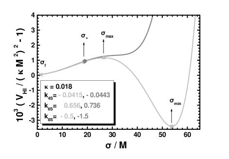
The structure of is displayed in Fig. 1 where we show the variation of as a function of for and (gray line) or (light gray line). These parameters yield , and (gray [light gray] line). The values of [] (gray [light gray] line) and are also depicted. In the first case (gray line) remains monotonic due to the larger value employed. Contrarily, develops the minimum-maximum structure, in the second case (light gray line) with the maximum located at and the minimum at – the values obtained via Eqs. (20a) and (20b) are indicated in curly brackets. We find that .
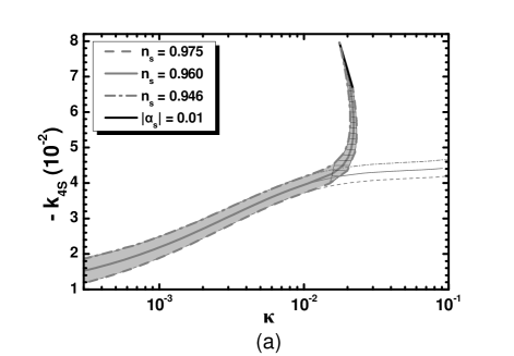
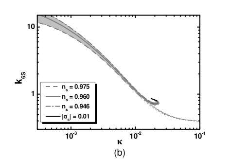
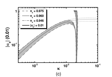
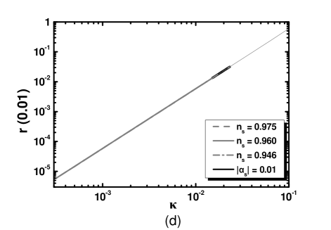
Confronting FHI with the constraints of Sec. III, we can identify the allowed regions in the , , and planes – see Fig. 2. The conventions adopted for the various lines are also shown. In particular, the thick and thin gray dashed [dot-dashed] lines correspond to [], whereas the thick and thin gray solid lines are obtained by fixing – see Eq. (15a). The thick lines are obtained setting which – together with the universally selected and above – ensures the fulfilment of restriction 6 of Sec. III; the faint lines correspond to the choice , which does not ensure the boundedness of . From the panels (a), (b) and (c) we see that the thin lines almost coincide with the thick ones for , and then deviate and smoothly approach some plateau. The regions allowed by imposing the constraints 1-6 of Sec. III are denoted by light gray shading. In the hatched subregions, requirement 7 is also met. On the other hand, the regions surrounded by the thin lines are actually the allowed ones, when only the restrictions 1-5 of Sec. III are satisfied. The various allowed regions are cut at low values since the required reaches rather high values (of order 10), which starts looking unnatural. At the other end, Eq. (16) and bounds the allowed areas in the case of bounded or unbounded respectively. For both cases, we remark that increases with whereas drops as increases. For fixed , increasing means decreasing . Moreover, is restricted to somewhat small values in order to avoid the well-known lectures ; review problem of FHI. On the other hand, no tuning for is needed since it is of order unity for most values.
From Fig. 2-(c) we observe that for increasing beyond , corresponding to the bold lines precipitously drops at , changes sign and rapidly saturates the bound of Eq. (16) along the thick black solid line. In other words, for every in the vicinity of we have two acceptable values, as shown in Fig. 2-(b) with two different values of either sign. Furthermore, from Fig. 2-(d) we remark that is largely independent of the value, and so the various types of lines coincide for both bound and unbounded . We also see that increases almost linearly with and reaches its maximal value which turns out to be: (i) as approaches the bound of Eq. (16), for bounded ; (ii) as the inequality is saturated for and unbounded . Therefore, lifting restriction 6 of Sec. III allows larger . However, non vanishing ’s perhaps corresponds to a more natural scenario.
We observe that the optimistic restriction 7 in Sec. III can be met in very limited slices of the allowed (lightly gray shaded) areas, only when the boundedness of has been ensured. In these regions also turns out to be rather large (), and we therefore observe a mild dependence of our results on (or ). This point is further clarified in Table 1 where we list the model parameters and predictions for , and various values. We remark that for the results are practically unchanged for varying . The dependence on starts to become relevant for and crucially affects the results for ; here, for the solution obtained belongs to the branch with and not in the branch with , as is the case with and . Listed is also the quantity which takes rather natural values for the selected – the entries without a value assigned indicate that is a monotonic function of .
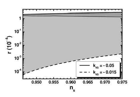
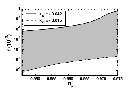
As shown in Fig. 2-(a), ranges between about and for the case with bounded or for unbounded . For each of these values and every in the allowed range found in Fig. 2, we vary in order to obtain in the observationally favored region of Eq. (15a) and we extract the resulting . Our results are presented in Fig. 3, where we display the allowed region in the plane for bounded (upper plot) or unbounded (lower plot) . Along the dashed lines of both plots ranges between and whereas along the solid line of the upper [lower] plot varies between and [ and ]. From the upper plot we see that the maximal for is about and turns out to be nearly independent of . Interestingly, this value is included in the region with monotonic depicted by the hatched region. From the lower plot we see that there is a mild dependence of the largest from ; thus, the maximal is achieved for . No region with monotonic is located in this case, however.
Summarizing our findings from Figs. 2 and 3 for in the range given by Eq. (15a) and imposing the restrictions 1-7 of Sec. III, the various quantities are bounded as follows:
| (21a) | |||
| (21b) | |||
| (21c) | |||
| (21d) | |||
| (21e) | |||
Note that the limiting values obtained without imposing the monotonicity of – requirement 7 in Sec. III – are indicated in curly brackets. In the corresponding region, ranges between and . As can be deduced from the data of Fig. 2, increases with ’s. Small values indicate a second mild tuning (besides the one needed to avoid the problem), which is however a common feature in the models of hilltop inflation. The predicted values are close to the lowest detectable tensor fraction through cosmic microwave background polarization referee ; these are thus virtually impossible to be observed experimentally. Possibly detectable values can be achieved if we ignore requirement 6 of Sec. III. Indeed, confining in the range of Eq. (15a) we obtain the following ranges:
| (22a) | |||
| (22b) | |||
| (22c) | |||
| (22d) | |||
| (22e) | |||
Obviously, no solutions with monotonic are achieved in this case whereas varies between and . The maximal is reached for the maximal in Eq. (15a) and as .
So far we focused on , employing in our investigation. However, our results are not drastically affected even in the case of for most values of , as can be inferred by comparing the results (for ) listed in Tables 1 and 2 where we use and respectively. This signals the fact that the SUGRA corrections to originating from the last term in the sum of Eq. (7) dominate over the radiative corrections which are represented by . The discrepancy between the two results ranges from to , increasing with , and it is essentially invisible in the plots of Fig. 2. On the other hand, we observe that in the case the enhanced creates a relatively wider space with monotonic ; this space is certainly smaller for , as shown from our outputs for .
V Conclusions
Inspired by the recently released results by the PLANCK collaboration on the inflationary observables, we have reviewed and updated the nonminimal version of SUSY hybrid inflation arising from F-terms, also referred to as FHI. In our formulation, FHI is based on a unique renormalizable superpotential, employs an quasi-canonical Kähler potential and is followed by the spontaneous breaking at of a GUT symmetry which is taken to be or . As suggested first in Ref. rlarge and further exemplified in Ref. hinova ; alp , values close to in conjunction with the fulfilment of Eq. (17) can be accommodated by considering an expansion of the Kähler potential – see Eq. (6) – up to twelfth order in powers of the various fields with suitable choice of signs for the coefficients and .
Fixing at its central value, we obtain with and , while and assume the values and respectively – recall that the limiting values in the curly brackets are achieved without imposing the monotonicity of . With a non-monotonic , ranges between and . It is gratifying that there is a sizable portion of the allowed parameter space where remains a monotonically increasing function of ; thus, unnatural restrictions on the initial conditions for inflation due to the appearance of a maximum and a minimum of can be avoided. On the other hand, if we do not insist on the boundedness of , reaches with and with the resulting and being both , that is close to . Finally FHI can be followed by a successful scenario of non-thermal leptogenesis lept for both ’s considered here – cf. Ref. flipped ; alp .
Note Added
After the completion of this work, the Bicep2 collaboration gws recently reported the discovery of B-mode polarization of the cosmic microwave background radiation. If this mode is attributed to the primordial gravity waves predicted by inflation, it implies gws – after subtraction of the various dust models – which is partially in tension with the WMAP and PLANCK results plin ; wmap – see Eq. (15b). Therefore, it is still premature to exclude any inflationary model with lower than the above limit. Moreover, the current data cannot definitively rule out other sources of gravitational waves – see e.g. Ref. dent . The inflationary models considered in this work yield values well below those required by Bicep2 results gws , especially for inflationary potentials bounded from below – see Eqs. (21e) and (22e). If the Bicep2 results are confirmed by other ongoing experiments, the present class of models defined by the superpotential in Eq. (1), the Kähler potential in Eq. (6) and the theoretical constraint in Eq. (17) can be categorically excluded.
Acknowledgments.
M.C. and Q.S. acknowledge support by the DOE grant No. DE-FG02-12ER41808. CP acknowledges support from the Generalitat Valenciana under grant PROMETEOII/2013/017.References
- (1)
References
K. Kumekawa, T. Moroi and T. Yanagida, Prog. Theor. Phys. 92, 437 (1994) [hep-ph/9405337]; G. Lazarides, R.K. Schaefer and Q. Shafi, Phys. Rev. D 56, 1324 (1997) [hep-ph/9608256]; V.N. Şenoğuz and Q. Shafi, Phys. Rev. D 71, 043514 (2005) [hep-ph/0412102].