Abstract

In a very simple stock market, made by only two initially equivalent traders, we discuss how the information can affect the performance of the traders. More in detail, we first consider how the portfolios of the traders evolve in time when the market is closed. After that, we discuss two models in which an interaction with the outer world is allowed. We show that, in this case, the two traders behave differently, depending on i) the amount of information which they receive from outside; and ii) the quality of this information.

I Introduction and motivations

In a series of papers, [1]-[4], one of us (FB) has shown how the Heisenberg time evolution used for quantum mechanical systems can be adopted in the analysis of some simplified stock markets. After these original applications, the same tools were also used for rather different macroscopic systems. A recent monograph on these topics is [5]. In the cited papers and in [5] the role of information was, in a certain sense, only incorporated by properly choosing some of the constants defining the Hamiltonian of the system we were considering.

On the other hand, the other author (EH), following the original idea of [6], considered the role of information for stock markets, [7]-[8], mainly adopting the Bohm view to quantum mechanics, where the information is carried by a pilot wave function $\Psi(x,t)$, satisfying a Schrödinger equation of motion, and which, with simple computations, produces what is called a mental force which has to be added to the other hard forces acting on the system, producing a full Newton-like classical differential equation.

In this paper we try first to incorporate the effect of this mental force at a purely quantum mechanical level. After that, we consider a simplified stock market, which, to simplify the notation, we consider with just two traders $\tau_{1}$ and $\tau_{2}$, describing what happens before the trading begins, i.e. in the phase in which the information begins to circulate in the market, and is used by the traders to decide their next moves. The rationale for focusing on the way information can influence valuation of portfolios is a very important topic in finance and economics. We stress that it is the modeling of the information which is at the heart of the problem in such valuation exercises. We believe this paper shows that tools from quantum mechanics can aid in a very valuable way to this modeling challenge.

It may be worth stressing that our analysis continues a nowadays rather rich literature on the role of quantum mechanics in economics, see [9]-[14] for instance, which shows that an increasing number of researchers believe that some of the aspects of a real stock market could be described by adopting tools and ideas coming from quantum mechanics. We should stress that, in our knowledge, the first paper where such a connection between quantum mechanics and finance appeared is [15], where the authors suggested that non commuting operators are really needed in the description of a realistic market to prevent exact knowledge of the price of a share and of its forward time derivative. See also [12]. These two quantities, in [12] and [15], were associated to operators having the same commutation rule as the position and the momentum operators in ordinary quantum mechanics, and therefore obey an uncertainty principle. Furthermore, there is scope to argue that for instance the central concept of non-arbitrage in finance has connections with hermiticity in quantum mechanics. Baaquie [12] has shown that the hamiltonian of the Black-Scholes equation is not hermitian. This non-existence of hermiticity is narrowly related to the absence of arbitrage (the existence of a martingale). Clearly, hermiticity on itself is not making anything quantum mechanical as such, but it is still an important argument. There are other interesting arguments, such as the way hidden variable theory can connect with the (non-observable) state prices, in again, the non-arbitrage theorem. See [16] Finally, we also want to mention that in the context of decision theory, notably in the resolving of some expected utility paradoxes, the use of quantum probability is very promising. Those paradoxes lie at the base of many economics/finance models. We document those achievements in [16]. In essence, the use of quantum mechanical techniques into social science revolve really around formalizing information. See [5].

The paper is organized as follows: in the next section we briefly discuss how the pilot wave function can be incorporated in our Heisenberg-like dynamics. Then, in Section III we introduce a first model of a closed market, where the information (or, in our setting, the lack of information, LoI in the following) will behave as the other operators, i.e., it will be described by ordinary two-modes bosonic operators. In Section IV we replace these operators with two families of bosonic operators, describing sources and sinks of information which modify, in the way described below, directly the portfolios of the traders. In Section V, finally, we consider a more complete model where the outer world contributes in the definition of the strategies of the traders in a more realistic way, i.e. by contributing to the information of the traders, rather than being the information by itself. Section VI contains our conclusions.

II Some preliminaries

In FB’s approach to stock markets the maybe crucial ingredient of the model is the Hamiltonian operator $H$ which is taken to describe the system. In [5] several useful rules have been proposed to fix the expression of $H$. We need now to incorporate in $H$ the effect described by the pilot wave function, extending, for instance, what is discussed in [17]. See also [6]. Let us recall here the essential steps: the main ingredient is the (two-dimensional, in our case) pilot wave function, $\Psi(q_{1},q_{2})$, which evolves in time according to the Schrödinger equation of motion

$$i\frac{\partial\Psi(q_{1},q_{2};t)}{\partial t}=\left[-\frac{\hbar^{2}}{2m}\sum_{j=1}^{2}\frac{\partial^{2}}{\partial q_{j}^{2}}+V(q_{1},q_{2})\right]\Psi(q_{1},q_{2};t),$$

where $\hbar$ and $m$ have a suitable economics based meaning, [6] and [17], and $V(q_{1},q_{2})$ is the potential due to the hard economics based effects. Then, calling $R(q_{1},q_{2})=|\Psi(q_{1},q_{2})|$, a new potential is constructed by defining $U(q_{1},q_{2})=-\frac{1}{R(q_{1},q_{2})}\sum_{j=1}^{2}\frac{\partial^{2}R(q_{1},q_{2})}{\partial q_{j}^{2}}$, and $U(q_{1},q_{2})$ produces the mental forces affecting the traders: $g_{j}(q_{1},q_{2})=-\frac{\partial U(q_{1},q_{2})}{\partial q_{j}}$, $j=1,2$. Please note the definition of this new potential is not foreign to physics but is squarely steeped into Bohmian mechanics (which is a particular interpretation of quantum mechanics). The key references are [18] and [19]. Finally, if we call $\pi_{j}(t)$ the value of the portfolio of $\tau_{j}$, its time evolution is driven by the following classical (Newtonian-like) differential equation:

$$\dot{\pi}_{j}(t)=-\frac{\partial V(q_{1},q_{2})}{\partial q_{j}}-\frac{\partial U(q_{1},q_{2})}{\partial q_{j}}=:f_{j}(q_{1},q_{2})+g_{j}(q_{1},q_{2}),$$

$j=1,2$, with obvious notation. Hence, the time evolution of $\pi_{j}(t)$ is governed by hard factors ($f_{j}$) as well as by the financial mental force $g_{j}$, [6, 17].

What is important for us is the potential $U(q_{1},q_{2})$, which represents, in some sense, the fact that $\tau_{1}$ and $\tau_{2}$ are reached by two, in general different, amounts of information. Therefore it is natural to assume that $U(q_{1},q_{2})=U_{1}(q_{1})+U_{2}(q_{2})$, with $U_{1}$ and $U_{2}$, in general, different functions of their arguments. In this way we can model, quite simply, the fact that $g_{1}=-\frac{\partial U}{\partial q_{1}}$ can be different from $g_{2}-\frac{\partial U}{\partial q_{2}}$ and, quite importantly from a technical point of view, the quantum-like Hamiltonian constructed out of this potential can be viewed as the sum of two one-body Hamiltonians, [20]. Just to fix the ideas, the Hamiltonian for the market will contain a contribution like this:

$$\Omega_{1}\,i_{1}^{\dagger}\,i_{1}+\Omega_{2}\,i_{2}^{\dagger}\,i_{2},$$

for closed systems, or having a slightly more general expression for open systems. Here $\Omega_{1}$ and $\Omega_{2}$ are positive numbers, while $i_{j}$’s are bosonic operators (i.e. $[i_{j},i_{k}^{\dagger}]=1\!\!1\delta_{j,k}$). This is exactly the kind of contribution one has for a two particle systems in ordinary quantum theory, when the free energies of the particles are expected to be different.

Remark:– It should be stressed that when we use above and in the sequel of this paper the terms closed or open systems, this terminology should be taken with a certain care. In fact, we call a system closed when the information is described by a two-modes bosonic operator, obeying the commutation rules above. In other words, information, cash and shares are operators exactly of the same kind. This will be made more explicit in the next sections. However, since we expect the information comes from outside the market, it would probably be more appropriate to speak of absence of reservoir.

The above remark is related to another interesting aspect of the models proposed here, which somehow look different from those considered in [1]-[4]. In these former papers, the cash and the number of shares of the traders were assumed to be constant in time: the shares are not created or destroyed, for instance. Here, on the contrary, we allow for such a possibility, so that bankruptcy can be discussed within our present scheme. Moreover, we are not even assuming that the cash is only used to buy shares, so that it needs not to be preserved in time, as well. However, we will see in the next sections that other observables will be constant, and we will see that these observables do have a clear economical meaning, indeed.

As already anticipated, in this paper we will be essentially interested not in the interaction between the traders, but rather in the effect of the outer world in preparing the system, i.e. in fixing the initial status of the various traders after they have been reached by the information but before they start to trade. For this reason, if we call $H_{full}=H+H_{ex}$ the Hamiltonian describing the traders and the information, and if with $H_{ex}$ we mean that part of $H_{full}$ describing the exchanges between $\tau_{1}$ and $\tau_{2}$, see [5], we will only be interested here in $H$. It is like if we are considering two different time intervals: in the first one, $[0,t_{1}]$, the two traders, which are indistinguishable at $t=0$, receive a different amount of information. This allows them to react in different ways, so that, at time $t_{1}$, they are expected to become different. In this interval, $H_{full}$ coincides with $H$. For $t>t_{1}$, the two traders have been prepared in different ways, and the Hamiltonian is now $H_{ex}$ (plus, in general, a free contribution). In other words, we could think of writing $H_{full}=H+\Theta(t-t_{1})\,H_{ex}$, where $\Theta(t)=1$ if $t>0$, while $\Theta(t)=0$ otherwise. Since, in this paper, we will only be interested in the first time interval, $[0,t_{1}]$, the role of $H_{ex}$ will not be very relevant here. We will say more on $H_{ex}$ in our conclusions. This approach has also a quite useful technical consequence: there is no real need, at this stage, to introduce the price of the share and to consider its dynamical behavior. This becomes really important, of course, when transactions are considered, not before. For this reason, in this paper, the price of the shares (just a single kind of shares!) will be fixed to be one. Again, we will say more on this in Section VI.

III A first model with no reservoir

The first model we want to consider is described by the following Hamiltonian:

$$\left\{\begin{array}[]{ll}H=H_{0}+H_{inf},&\\ H_{0}=\sum_{j=1}^{2}(\omega_{j}^{s}\hat{S}_{j}+\omega_{j}^{c}\hat{K}_{j}+\Omega_{j}\hat{I}_{j}),&\\ H_{inf}=\lambda_{inf}\sum_{j=1}^{2}\left(i_{j}(s_{j}^{\dagger}+c_{j}^{\dagger})+i_{j}^{\dagger}(s_{j}+c_{j})\right).&\end{array}\right.$$ (3.1)

Here $\hat{S}_{j}:=s_{j}^{\dagger}s_{j}$, $\hat{K}_{j}:=c_{j}^{\dagger}c_{j}$, and $\hat{I}_{j}:=i_{j}^{\dagger}i_{j}$, $j=1,2$. The following canonical commutation relations (CCRs) are assumed:

$$[s_{j},s_{k}^{\dagger}]=[c_{j},c_{k}^{\dagger}]=[i_{j},i_{k}^{\dagger}]=\delta_{j,k}1\!\!1,$$ (3.2)

where $1\!\!1$ is the identity operator. All the other commutators are zero.

The meaning of these operators is widely discussed in [5]: $s_{j}$ destroys a share in the portfolio of $\tau_{j}$, see below, while $s_{j}^{\dagger}$ creates a share. The operators $c_{j}$ and $c_{j}^{\dagger}$ respectively lower and rise the amount of cash of $\tau_{j}$. Finally, $i_{j}^{\dagger}$ increases the LoI of $\tau_{j}$, while $i_{j}$ decreases it. Therefore, the meaning of $H_{inf}$ is the following: whenever the LoI decreases (because of $i_{j}$), the value of the portfolio operator of $\tau_{j}$, $\hat{\pi}_{j}:=\hat{S}_{j}+\hat{K}_{j}$ , increases (because of $s_{j}^{\dagger}+c_{j}^{\dagger}$). Of course, since $H_{inf}$ also contains the adjoint contribution $i_{j}^{\dagger}(s_{j}+c_{j})$, if the LoI increases, then $\hat{\pi}_{j}$ decreases.

It is not hard to check that, calling $\hat{M}_{j}:=\hat{S}_{j}+\hat{K}_{j}+\hat{I}_{j}=\hat{\pi}_{j}+\hat{I}_{j}$, the following is true: $[H,\hat{M}_{j}]=0$, $j=,1,2$. Consequently, even if the cash and the shares are not separately preserved, the sum of the portfolio and the LoI of each trader (and therefore of the whole market) stays constant. This has an economical meaning: whenever the LoI increases, it is natural to imagine that the value of the portfolio of the related trader should decrease, while having more information means having more chances to increase one’s wealth. And this is exactly what the commutativity between $H$ and $\hat{M}_{j}$ implies.

The equation of motion for $\tau_{j}$ can be easily deduced using the Heisenberg equation of motion $\dot{X}(t)=i[H,X(t)]$. We find that

$$\dot{X}_{j}(t)=-iT_{j}X_{j}(t),$$ (3.3)

where

$$X_{j}(t)=\left(\begin{array}[]{c}s_{j}(t)\\ c_{j}(t)\\ i_{j}(t)\\ \end{array}\right),\qquad T_{j}=\left(\begin{array}[]{ccc}\omega_{j}^{s}&0&\lambda_{inf}\\ 0&\omega_{j}^{c}&\lambda_{inf}\\ \lambda_{inf}&\lambda_{inf}&\Omega_{j}\\ &&\end{array}\right).$$ (3.4)

The solution can be written as $X_{j}(t)=V_{j}(t)X_{j}(0)$, where $V_{j}(t)=U_{j}\Sigma_{j}(t)U_{j}^{-1}$, $U_{j}$ being the matrix which diagonalizes $T_{j}$, $U_{j}^{-1}T_{j}U_{j}=diag\{\sigma_{1}^{(j)},\sigma_{2}^{(j)},\sigma_{3}^{(j)}\}=:\sigma_{j}$, and $\Sigma_{j}(t)=\exp\{-i\,\sigma_{j}\,t\}=\left(\begin{array}[]{ccc}e^{-i\sigma_{1}^{(j)}t}&0&0\\ 0&e^{-i\sigma_{2}^{(j)}t}&0\\ 0&0&e^{-i\sigma_{3}^{(j)}t}\end{array}\right)$.

The state of the system, at $t=0$, is assumed to be $\varphi_{\mathcal{G}}:=\varphi_{S_{1},K_{1},I_{1},S_{2},K_{2},I_{2}}$, which, see [5], can be constructed by a vacuum $\varphi_{\mathbf{0}}$, $c_{j}\varphi_{\mathbf{0}}=s_{j}\varphi_{\mathbf{0}}=i_{j}\varphi_{\mathbf{0}}=0$, $j=1,2$, acting with powers of the raising operators $c_{j}^{\dagger}$, $s_{j}^{\dagger}$ and $i_{j}^{\dagger}$, and normalizing the result. The vector $\varphi_{\mathcal{G}}$ describes a market in which, at $t=0$, $\tau_{1}$ possesses $S_{1}$ shares, $K_{1}$ units of cash, and is affected by a LoI equal to $I_{1}$. Similarly for $\tau_{2}$. The time evolution of the cash of $\tau_{j}$ is deduced by computing $N_{K_{j}}(t):=\left<\varphi_{\mathcal{G}},c_{j}^{\dagger}(t)c_{j}(t)\varphi_{\mathcal{G}}\right>$. Analogously, the number of shares are given by $N_{S_{j}}(t):=\left<\varphi_{\mathcal{G}},s_{j}^{\dagger}(t)s_{j}(t)\varphi_{\mathcal{G}}\right>$. The value of the portfolio of $\tau_{j}$ is just the sum of $N_{K_{j}}(t)$ and $N_{S_{j}}(t)$:

$$\pi_{j}(t)=\left<\varphi_{\mathcal{G}},\hat{\pi}_{j}(t)\varphi_{\mathcal{G}}\right>=N_{S_{j}}(t)+N_{K_{j}}(t).$$ (3.5)

In the previous analysis carried out by one of us (FB), it was suggested that the parameters of the free Hamiltonians influence significantly the interacting system, while they play no role if no interaction occurs. The same conclusion also follows from the analysis carried out here. To put in evidence this aspect, it is better to choose $\tau_{1}$ completely equivalent to $\tau_{2}$: hence we fix, first of all, $S_{1}=S_{2}$, $K_{1}=K_{2}$, $I_{1}=I_{2}$. This means that the initial conditions of the two traders are identical. Moreover, we also ask that $\lambda_{inf}=0.5$ (just to fix the ideas) and that $\omega_{1}^{s}=\omega_{2}^{s}=:\omega^{s}$, $\omega_{1}^{c}=\omega_{2}^{c}=:\omega^{c}$ and $\Omega_{1}=\Omega_{2}$. Therefore, the Hamiltonian for $\tau_{1}$ is identical to the one for $\tau_{2}$. This implies that the matrix $T_{j}$ in (3.4) for the two traders are equal: $T_{1}=T_{2}$ and, clearly, the portfolios of the two traders coincide during their time evolution: $\pi_{1}(t)=\pi_{2}(t)=:\pi(t)$. What appears interesting to us is that the higher the values of $\omega^{s}$ and $\omega^{c}$, the smaller the amplitude of the oscillations of the portfolios: as in very different systems, [5], in this simple situation, the parameters of the free Hamiltonian behave as a sort of inertia for the traders, restricting more and more the widths of the oscillations. In Figure 1 we plot $\pi(t)$ for $S_{1}=30$, $K_{1}=15$ and $I_{1}=5$, and for $\omega^{s}=\omega^{c}=20$, $\Omega_{1}=\Omega_{2}=3$ (left), and for $\omega^{s}=\omega^{c}=2$, $\Omega_{1}=\Omega_{2}=3$ (right). We see in both cases oscillation of $\pi(t)$, but the range (and the frequencies) of the oscillations are quite different in the two cases.

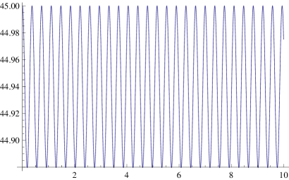
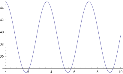
Figure 1: $\pi(t)$ for $\omega^{s}=\omega^{c}=20$ (left) and $\omega^{s}=\omega^{c}=2$ (right)

Let us now consider the case in which the two traders, originally (i.e. at $t=0$) prepared in the same way ($S_{1}=S_{2}=30$, $K_{1}=K_{2}=15$, $I_{1}=I_{2}=5$), are no longer completely equivalent: again we put $\omega_{1}^{s}=\omega_{2}^{s}=:\omega^{s}$ and $\omega_{1}^{c}=\omega_{2}^{c}=:\omega^{c}$, but we now assume that $\Omega_{1}>\Omega_{2}$. In particular, in Figure 2 we plot $\pi_{1}(t)$ (left) and $\pi_{2}(t)$ (right) for the choices $\omega^{s}=1$, $\omega^{c}=2$, $\Omega_{1}=5$ and $\Omega_{2}=1$. In Figure 3 the parameters are $\omega^{s}=1$, $\omega^{c}=2$, $\Omega_{1}=10$ and $\Omega_{2}=1$.

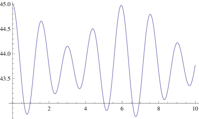
Figure 2: $\pi_{1}(t)$ (left) and $\pi_{2}(t)$ (right) for $\omega^{s}=1$, $\omega^{c}=2$, $\Omega_{1}=5$ and $\Omega_{2}=1$

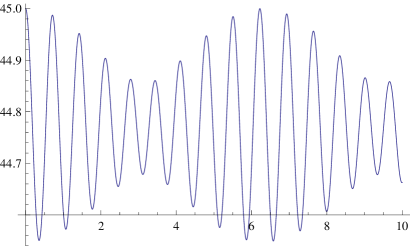
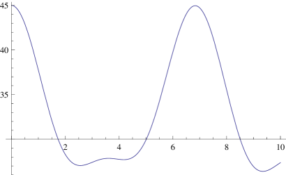
Figure 3: $\pi_{1}(t)$ (left) and $\pi_{2}(t)$ (right) for $\omega^{s}=1$, $\omega^{c}=2$, $\Omega_{1}=10$ and $\Omega_{2}=1$

We see again that, increasing $\Omega_{1}$ produces a smaller amplitude of oscillation (bigger inertia) and a larger frequency. In fact, it is also evident from Figures 1-3 that the omega’s affect the (pseudo-)frequencies of the functions $\pi_{j}(t)$: it seems that a larger loss of information induces more frequent changes in portfolio values.

From both figures it is evident how the values of the free Hamiltonian do in fact play a relevant role in the time evolution of the interacting system. This is interesting since, if we take $\lambda_{inf}=0$, then both $\pi_{1}(t)$ and $\pi_{2}(t)$ turn out to stay constant in time: no information $\Rightarrow$ no action!

Rather than considering other aspects of this model, we consider now a different, and more interesting Hamiltonian, based on the idea that the LoI is related to the outer world surrounding the traders (the rumors, the news, facts, etc.).

IV The reservoir is the information

The Hamiltonian we are interested in here is simply a generalized version of that introduced in the previous section. The main difference is that the two pairs of lack-of-information operators, $(i_{1},i_{1}^{\dagger})$ and $(i_{2},i_{2}^{\dagger})$, are replaced by two families of similar operators, labeled by the real numbers: $(i_{1}(k),i_{1}^{\dagger}(k))$ and $(i_{2}(k),i_{2}^{\dagger}(k))$, where $k\in\mathbb{R}$ could be viewed as a wave number, satisfying the commutation rules

$$[i_{n}(k),i_{m}^{\dagger}(q)]=\delta_{n,m}\delta(k-q)1\!\!1,$$

all the other commutators being zero. The Hamiltonian is now

$$\left\{\begin{array}[]{ll}H=H_{0}+H_{inf},&\\ H_{0}=\sum_{j=1}^{2}(\omega_{j}^{s}\hat{S}_{j}+\omega_{j}^{c}\hat{K}_{j}+\int_{\mathbb{R}}\Omega_{j}(k)\hat{I}_{j}(k)\,dk),&\\ H_{inf}=\lambda_{inf}\sum_{j=1}^{2}\int_{\mathbb{R}}\left(i_{j}(k)(s_{j}^{\dagger}+c_{j}^{\dagger})+i_{j}^{\dagger}(k)(s_{j}+c_{j})\right)\,dk.&\end{array}\right.$$ (4.1)

Once again, the model admits some integrals of motion: $\hat{M}_{j}:=\hat{S}_{j}+\hat{K}_{j}+\hat{I}_{j}=\hat{\pi}_{j}+\hat{I}_{j}$, where $\hat{\pi}_{j}=\hat{S}_{j}+\hat{K}_{j}$ is, as before, the portfolio operator for $\tau_{j}$ and $\hat{I}_{j}=\int_{\mathbb{R}}\hat{I}_{j}(k)\,dk$ is its full LoI. The existence of these integrals of motion have the same economical meaning we have already discussed in the previous section, and this will not be repeated here.

The Heisenberg equations of motion for the operators of $\tau_{j}$ can be easily found:

$$\left\{\begin{array}[]{ll}\frac{d}{dt}s_{j}(t)=-i\omega_{j}^{s}s_{j}(t)-i\lambda_{inf}\int_{\mathbb{R}}i_{j}(k,t)\,dk,&\\ \frac{d}{dt}c_{j}(t)=-i\omega_{j}^{c}c_{j}(t)-i\lambda_{inf}\int_{\mathbb{R}}i_{j}(k,t)\,dk,&\\ \frac{d}{dt}i_{j}(k,t)=-i\Omega_{j}(k)i_{j}(k,t)-i\lambda_{inf}(s(t)+c(t)).&\end{array}\right.$$ (4.2)

We will solve this system under the simplifying assumption that $\omega_{j}^{s}=\omega_{j}^{c}=:\omega_{j}$. This is technically convenient, since in this case the system above can be replaced by the simpler set of equations

$$\left\{\begin{array}[]{ll}\frac{d}{dt}c_{j}(t)=-i\omega_{j}c_{j}(t)-i\lambda_{inf}\int_{\mathbb{R}}i_{j}(k,t)\,dk,&\\ \frac{d}{dt}i_{j}(k,t)=-i\Omega_{j}(k)i_{j}(k,t)-i\lambda_{inf}(2c_{j}(t)+e^{-i\omega_{j}t}(s_{j}(o)-c_{j}(0))).&\end{array}\right.$$ (4.3)

It is well known how to proceed in this case, [5]: we first rewrite the second equation in integral form, and then we replace this formula in the first equation above. Now, assuming that $\Omega_{j}(k)=\Omega_{j}\,k$ for some positive $\Omega_{j}$, and recalling that $\int_{\mathbb{R}}e^{-i\Omega_{j}\,k(t-t_{1})}\,dk=\frac{2\pi}{\Omega_{j}}\delta(t-t_{1})$ and that, for suitable $g(t)$, $\int_{0}^{t}g(t_{1})\delta(t-t_{1})\,dt_{1}=\frac{1}{2}g(t)$, after some standard computations we deduce that

$$c_{j}(t)=e^{-\left(i\omega_{j}+\frac{2\pi\lambda_{inf}^{2}}{\Omega_{j}}\right)t}\times$$

$$\times\left[\frac{1}{2}c_{j}(0)\left(1+e^{\frac{2\pi\lambda_{inf}^{2}}{\Omega_{j}}t}\right)-\frac{1}{2}s_{j}(0)\left(e^{\frac{2\pi\lambda_{inf}^{2}}{\Omega_{j}}t}-1\right)-i\lambda_{inf}\int_{\mathbb{R}}i_{j}(k)\eta_{j}^{(1)}(k,t)dk\right].$$ (4.4)

Here we have defined the function

$$\eta_{j}^{(1)}(k,t)=\frac{1}{i(\omega_{j}-\Omega_{j}\,k)+\frac{2\pi\lambda_{inf}^{2}}{\Omega_{j}}}\left(\exp\left\{\left(i(\omega_{j}-\Omega_{j}\,k)+\frac{2\pi\lambda_{inf}^{2}}{\Omega_{j}}\right)t\right\}-1\right).$$

What we are interested in, as in the previous section, is, first of all, the mean value of $\hat{K}_{j}(t)=c_{j}^{\dagger}(t)c_{j}(t)$ on a state $\left<.\right>$ over the whole system, i.e. a state over the traders and their reservoirs. For each operator of the form $X_{sm}\otimes Y_{res}$, $X_{sm}$ being an operator of the stock market and $Y_{res}$ an operator of the reservoir, we have

$$\left\langle X_{sm}\otimes Y_{res}\right\rangle:=\left\langle\varphi_{\mathcal{G}},X_{sm}\varphi_{\mathcal{G}}\right\rangle\,\omega_{res}(Y_{res}).$$

Here $\varphi_{\mathcal{G}}$ is defined in analogy with the vectors introduced in the previous section, $\varphi_{\mathcal{G}}=\varphi_{S_{1},K_{1},S_{2},K_{2}}$, while $\omega_{res}(.)$ is a state satisfying the standard properties, [5],

$$\omega_{res}(1\!\!1_{res})=1,\quad\omega_{res}(i_{j}(k))=\omega_{res}(i_{j}^{\dagger}(k))=0,\quad\omega_{res}(i_{j}^{\dagger}(k)i_{l}(q))=N_{j}^{(I)}(k)\,\delta_{j,l}\delta(k-q),$$

for a suitable function $N_{j}^{(I)}(k)$. Also, $\omega_{res}(i_{j}(k)i_{l}(q))=0$, for all $j$ and $l$. Then we find

$$N_{K_{j}}(t):=\left\langle c_{j}^{\dagger}(t)c_{j}(t)\right\rangle=e^{-\frac{4\pi\lambda_{inf}^{2}}{\Omega_{j}}\,t}\times$$ (4.5)

$$\times\left[\frac{1}{4}N_{K_{j}}(0)\left(1+e^{\frac{2\pi\lambda_{inf}^{2}}{\Omega_{j}}t}\right)^{2}+\frac{1}{4}N_{S_{j}}(0)\left(e^{\frac{2\pi\lambda_{inf}^{2}}{\Omega_{j}}t}-1\right)^{2}+\lambda_{inf}^{2}\int_{\mathbb{R}}N_{j}^{(I)}(k)|\eta_{j}^{(1)}(k,t)|^{2}dk\right],$$

where we have introduced, in analogy with $N_{K_{j}}$, $N_{S_{j}}(t):=\left\langle s_{j}^{\dagger}(t)s_{j}(t)\right\rangle$. Using now the fact that $s_{j}(t)=c_{j}(t)+e^{-i\omega_{j}\,t}(s_{j}(0)-c_{j}(0))$, we can also deduce the time evolution of $N_{S_{j}}(t)$, which turns out to be

$$N_{S_{j}}(t)=N_{K_{j}}(t)+e^{-\frac{2\pi\lambda_{inf}^{2}}{\Omega_{j}}\,t}\left(N_{S_{j}}(0)\left(1-e^{\frac{2\pi\lambda_{inf}^{2}}{\Omega_{j}}\,t}\right)-N_{K_{j}}(0)\left(1+e^{\frac{2\pi\lambda_{inf}^{2}}{\Omega_{j}}\,t}\right)\right)+$$

$$+N_{K_{j}}(0)+N_{S_{j}}(0).$$ (4.6)

It is now easy to deduce the asymptotic behavior of the portfolio $\pi_{j}(t)=N_{K_{j}}(t)+N_{S_{j}}(t)$. After some computation, and assuming that $N_{j}^{(I)}(k)=N_{j}^{(I)}$ is constant in $k$, we deduce that

$$\delta\pi_{j}:=\lim_{t\rightarrow\infty}\pi_{j}(t)-\pi_{j}(0)=-\frac{1}{2}\pi_{j}(0)+2\lambda_{inf}^{2}\Omega_{j}^{2}\,N_{j}^{(I)}\int_{\mathbb{R}}\frac{dk}{4\pi^{2}\lambda_{inf}^{4}+\Omega_{j}^{2}(\omega_{j}-\Omega_{j}k)^{2}}.$$

The integral can be computed using standard complex techniques, and we end up with the following result

$$\delta\pi_{j}=-\frac{1}{2}\pi_{j}(0)+N_{j}^{(I)}.$$ (4.7)

In our idea, this conclusion is not particularly meaningful, since it states that between $\tau_{1}$ and $\tau_{2}$, the one who is better prepared, is the one who starts with a smaller portfolio and for which the associated reservoir has a larger value of $N_{j}^{(I)}$: if, for instance, $\pi_{1}(0)=\pi_{2}(0)$ and $N_{1}^{(I)}>N_{2}^{(I)}$, then $\delta\pi_{1}>\delta\pi_{2}$.

What it is not very satisfying to us is the fact that, apparently, the parameters of $H$ do not play any role in the behavior of the portfolios of the traders, at least on a long time scale. This suggests that the model should be improved further, and this is in fact the content of the next section.

V The reservoir generates the information

This section is devoted to a different, and probably more interesting model where the reservoir, rather than being directly linked to the LoI, is used to generate the information reaching the traders. More in detail, the Hamiltonian is

$$\left\{\begin{array}[]{ll}H=H_{0}+H_{int},&\\ H_{0}=\sum_{j=1}^{2}(\omega_{j}^{s}\hat{S}_{j}+\omega_{j}^{c}\hat{K}_{j}+\Omega_{j}\hat{I}_{j}+\int_{\mathbb{R}}\Omega_{j}^{(r)}(k)\hat{R}_{j}(k)\,dk),&\\ H_{int}=\sum_{j=1}^{2}\left[\lambda_{inf}\left(i_{j}(s_{j}^{\dagger}+c_{j}^{\dagger})+i_{j}^{\dagger}(s_{j}+c_{j})\right)+\gamma_{j}\int_{\mathbb{R}}(i_{j}^{\dagger}r_{j}(k)+i_{j}r_{j}^{\dagger}(k))\,dk\right],&\end{array}\right.$$ (5.1)

where $\hat{R}_{j}(k)=r_{j}^{\dagger}(k)r_{j}(k)$, $\hat{S}_{j}$, $\hat{K}_{j}$ and $\hat{I}_{j}$ are defined as in Section III, and the following CCRs are assumed,

$$[s_{j},s_{k}^{\dagger}]=[c_{j},c_{k}^{\dagger}]=[i_{j},i_{k}^{\dagger}]=1\!\!1\delta_{j,k},\quad[r_{j}(k),r_{l}^{\dagger}(q)]=1\!\!1\delta_{j,l}\delta(k-q),$$

all the other commutators being zero. The reservoir is described here by the operators $r_{j}(k)$, $r_{j}^{\dagger}(k)$ and $\hat{R}_{j}(k)$, and it is used to model the set of all the rumors, news, and external facts which, all together, create the final information. This Hamiltonian contains a free canonical part $H_{0}$, while the two contributions in $H_{int}$ respectively describe: (i) the same mechanism considered in Section III: when the LoI increases, the value of the portfolio decreases and vice-versa; (ii) the LoI increases when the ”value” of the reservoir decreases, and viceversa. Considering, for instance, the contribution $i_{j}r_{j}^{\dagger}(k)$ in $H_{int}$ we see that the LoI decreases (so that the trader is better informed) when a larger amount of news, rumors, etc. reaches the trader. Once again, no interaction between $\tau_{1}$ and $\tau_{2}$ is considered in (5.1), since this is not the main aim of this paper.

As in the previous models, some self-adjoint operators are preserved during the time evolution. These operators are $\hat{M}_{j}=\hat{S}_{j}+\hat{K}_{j}+\hat{I}_{j}+\hat{R}_{j}=\hat{\pi}_{j}+\hat{I}_{j}+\hat{R}_{j}$, $j=1,2$. Here the only new operator, with respect to those introduced in Section III, is $\hat{R}_{j}=\int_{\mathbb{R}}r_{j}^{\dagger}(k)r_{j}(k)\,dk$. Then we can check that $[H,\hat{M}_{j}]=0$, $j=1,2$. This implies that what is constant in time is the sum of the portfolio, the LoI and of the reservoir input of each single trader. Once again, there is no general need, and in fact it is not required, for the cash or the number of shares to be constant in time.

The Heisenberg differential equations of motion can now be easily deduced:

$$\left\{\begin{array}[]{ll}\frac{d}{dt}s_{j}(t)=-i\omega_{j}^{s}s_{j}(t)-i\lambda_{inf}\,i_{j}(t),&\\ \frac{d}{dt}c_{j}(t)=-i\omega_{j}^{c}c_{j}(t)-i\lambda_{inf}\,i_{j}(t),&\\ \frac{d}{dt}i_{j}(t)=-i\Omega_{j}i_{j}(t)-i\lambda_{inf}(s_{j}(t)+c_{j}(t))-i\gamma_{j}\int_{\mathbb{R}}r_{j}(k,t)\,dk&\\ \frac{d}{dt}r_{j}(k,t)=-i\Omega_{j}^{(r)}(k)\,r_{j}(k,t)-i\gamma_{j}\,i_{j}(t).&\end{array}\right.$$ (5.2)

In the previous section, to simplify the treatment, we required that $\omega_{j}^{s}=\omega_{j}^{c}$. However, also in view of the results we have deduced, we will avoid making this assumption now. We do not give the details of the solution of this system here, details which can be deduced by [5]. We just discuss the main steps. First of all, we rewrite the last equation in its integral form:

$$r_{j}(k,t)=r_{j}(k)e^{-i\Omega_{j}^{(r)}(k)t}-i\gamma_{j}\int_{0}^{t}i_{j}(t_{1})e^{-i\Omega_{j}^{(r)}(k)(t-t_{1})}\,dt_{1},$$

and we replace this in the differential equation for $i_{j}(t)$. Assuming that $\Omega_{j}^{(r)}(k)=\Omega_{j}^{(r)}\,k$, and proceeding as in the previous section, we deduce that

$$\frac{d}{dt}i_{j}(t)=-\left(i\Omega_{j}+\frac{\pi\gamma_{j}^{2}}{\Omega_{j}^{(r)}}\right)i_{j}(t)-i\gamma_{j}\int_{\mathbb{R}}r_{j}(k)e^{-i\Omega_{j}^{(r)}\,kt}\,dk-i\lambda_{inf}(s_{j}(t)+c_{j}(t)).$$ (5.3)

In the rest of this section we will work under the assumption that the last contribution in this equation can be neglected, when compared to the other ones. In other words, we are taking $\lambda_{inf}$ to be very small. However, our procedure is slightly better than simply considering $\lambda_{inf}=0$ in $H$ above, since we will keep the effects of this term in the first two equations in (5.2). Solving now (5.3) in its simplified expression, and replacing the solution $i_{j}(t)$ in the first equation in (5.2), we find:

$$s_{j}(t)=e^{-i\omega_{j}^{s}t}\left(s_{j}(0)-i\lambda_{inf}\alpha_{j}(t)\,i_{j}(0)-\lambda_{inf}\gamma_{j}\int_{\mathbb{R}}r_{j}(k)\,\eta_{2,j}(k,t)\,dk\right),$$ (5.4)

where we have defined

$$\alpha_{j}(t)=\frac{e^{(i\omega_{j}^{s}-\Gamma_{j})t}-1}{i\omega_{j}^{s}-\Gamma_{j}},\qquad\eta_{2,j}(k,t)=\int_{0}^{t}\eta_{1,j}(k,t_{1})e^{(i\omega_{j}^{s}-\Gamma_{j})t_{1}}\,dt_{1},$$

with

$$\Gamma_{j}=i\Omega_{j}+\frac{\pi\gamma_{j}^{2}}{\Omega_{j}^{(r)}},\qquad\eta_{1,j}(k,t)=\frac{e^{(\Gamma_{j}-i\Omega_{j}^{(r)}k)t}-1}{\Gamma_{j}-i\Omega_{j}^{(r)}k}.$$

It is clear from (5.2) that a completely analogous solution can be deduced for $c_{j}(t)$. The only difference is that $\omega_{j}^{s}$ should be replaced everywhere by $\omega_{j}^{c}$.

The states of the system extend those of the previous section: for each operator of the form $X_{sm}\otimes Y_{res}$, where $X_{sm}$ is an operator of the stock market and $Y_{res}$ an operator of the reservoir, we have

$$\left\langle X_{sm}\otimes Y_{res}\right\rangle=\left\langle\varphi_{\mathcal{G}},X_{sm}\varphi_{\mathcal{G}}\right\rangle\,\omega_{res}(Y_{res}).$$

Here $\varphi_{\mathcal{G}}$ is of the form $\varphi_{\mathcal{G}}=\varphi_{S_{1},K_{1},I_{1},S_{2},K_{2},I_{2}}$, exactly as in Section III, while $\omega_{res}(.)$ is a state satisfying again

$$\omega_{res}(1\!\!1_{res})=1,\quad\omega_{res}(r_{j}(k))=\omega_{res}(r_{j}^{\dagger}(k))=0,\quad\omega_{res}(r_{j}^{\dagger}(k)r_{l}(q))=N_{j}^{(r)}(k)\,\delta_{j,l}\delta(k-q),$$

for a suitable function $N_{j}^{(r)}(k)$, as in Section IV. Also, $\omega_{res}(r_{j}(k)r_{l}(q))=0$, for all $j$ and $l$. Then $N_{S_{j}}(t)=\left\langle s_{j}^{\dagger}(t)s_{j}(t)\right\rangle$ assumes the following expression:

$$N_{S_{j}}(t)=N_{S_{j}}(0)+\lambda_{inf}^{2}N_{I_{j}}(0)|\alpha_{j}(t)|^{2}+\lambda_{inf}^{2}\gamma_{j}^{2}\int_{\mathbb{R}}N_{j}^{(r)}(k)|\eta_{2,j}(k,t)|^{2}\,dk,$$ (5.5)

where $N_{I_{j}}(0)=\left\langle i_{j}^{\dagger}(0)i_{j}(0)\right\rangle=I_{j}$ and $N_{S_{j}}(0)=S_{j}$ are fixed by the quantum numbers of $\varphi_{\mathcal{G}}$. The expression for $N_{K_{j}}(t)=\left\langle c_{j}^{\dagger}(t)c_{j}(t)\right\rangle$ is completely analogous to the one above, with $\omega_{j}^{s}$ replaced by $\omega_{j}^{c}$, and the portfolio of $\tau_{j}$, $\pi_{j}(t)$, is simply the sum of $N_{S_{j}}(t)$ and $N_{K_{j}}(t)$. What we are interested in, is the variation of $\pi_{j}(t)$ over long time scales:

$$\delta\pi_{j}:=\lim_{t,\infty}\pi_{j}(t)-\pi_{j}(0).$$

Formula (5.5) shows that, if $\gamma_{j}$ is small enough, the integral contribution is expected not to contribute much to $\delta\pi_{j}$. For this reason, we will not consider it in the rest of the section. We now find

$$\delta\pi_{j}=\lambda_{inf}^{2}I_{j}(\Omega_{j}^{(r)})^{2}\left(\frac{1}{\pi^{2}\gamma_{j}^{4}+(\omega_{j}^{s}-\Omega_{j})^{2}(\Omega_{j}^{(r)})^{2}}+\frac{1}{\pi^{2}\gamma_{j}^{4}+(\omega_{j}^{c}-\Omega_{j})^{2}(\Omega_{j}^{(r)})^{2}}\right).$$ (5.6)

Let us now recall that, at $t=0$, the two traders are equivalent: $\omega_{1}^{c}=\omega_{2}^{c}=:\omega^{c}$, $\omega_{1}^{s}=\omega_{2}^{s}=:\omega^{s}$, $\Omega_{1}^{(r)}=\Omega_{2}^{(r)}$ and the initial conditions are $S_{1}=S_{2}$, $K_{1}=K_{2}$ and $I_{1}=I_{2}$. The main difference between $\tau_{1}$ and $\tau_{2}$ is in $\Omega_{1}$ which is taken larger than $\Omega_{2}$: $\Omega_{1}>\Omega_{2}$. With this in mind, we will consider three different cases: (a) $\gamma_{1}=\gamma_{2}$; (b) $\gamma_{1}>\gamma_{2}$; (c) $\gamma_{1}<\gamma_{2}$. In other words, we are allowing a different interaction strength between the reservoir and the information term in $H$.

Let us consider the first situation (a): $\gamma_{1}=\gamma_{2}$ and $\Omega_{1}>\Omega_{2}$. In this case it is possible to check that $\delta\pi_{1}<\delta\pi_{2}$, at least if $|\omega^{c}-\Omega_{2}|<|\omega^{c}-\Omega_{1}|$ and $|\omega^{s}-\Omega_{2}|<|\omega^{s}-\Omega_{1}|$. Notice that these inequalities are surely satisfied in our present assumptions if $\Omega_{1}$ and $\Omega_{2}$ are sufficiently larger than $\omega^{c}$ and $\omega^{s}$. In this case the conclusion is, therefore, that the larger the LoI, the smaller the increment in the value of the portfolio. Needless to say, this is exactly what we expected to find in our model. Exactly the same conclusion is deduced in case (b): $\gamma_{1}>\gamma_{2}$ and $\Omega_{1}>\Omega_{2}$. In this case the two inequalities produce the same consequences: we are doubling the sources of the LoI (one from $H_{0}$ and one from the interaction), and this implies a smaller increment of $\pi_{1}$. Case (c): $\gamma_{1}<\gamma_{2}$ and $\Omega_{1}>\Omega_{2}$, is different. In this case, while $H_{0}$ implies that $\tau_{1}$ is less informed (or that the quality of his information is not good enough), the inequality $\gamma_{1}<\gamma_{2}$ would imply exactly the opposite. The conclusion is that, for fixed $\Omega_{1}$ and $\Omega_{2}$, there exists a critical value of $(\gamma_{1},\gamma_{2})$ such that, instead of having $\delta\pi_{1}<\delta\pi_{2}$, we will have exactly the opposite inequality, $\delta\pi_{1}>\delta\pi_{2}$.

We should remind that these conclusions have been deduced under two simplifying assumptions which consist in neglecting the last contributions in (5.3) and in (5.5). Of course, to be more rigorous, we should also have some control on these approximations. However, we will not do this here.

As we see, this model is realistic and more than reasonable. Moreover, it might be worth to stress that in all the models considered in this paper, since the two traders do not interact with each other but only with the information, there is absolutely no need to limit the system to a simple two-traders stock market. In other words, as far as we are interested in the preliminary phase of the market, the interval $[0,t_{1}]$ introduced in Section II, we can easily extend all our models and our conclusions to larger markets, with an arbitrarily large number of traders.

VI Conclusions

In this paper we have proposed several models to incorporate the role of the information in a simplified, quantum-like, model of a stock market. In particular, we have considered what happens before the traders begin to interact, i.e. in a phase where the traders, identical at time $t=0$, begin to experience some information coming from inside the system (Section III) or from some surrounding world (Sections IV and V). Each one of the proposed models produce an interesting dynamical behavior, and the last one, in particular, appears to be quite promising for a deeper analysis.

The natural Step 2 of our research would consist in the analysis of what happens to the traders of a market prepared as, say, in Section V, when they start to interact, i.e. to buy and sell shares. Of course, the natural choice of the exchange Hamiltonian $H_{ex}$ introduced in Section II is the following, see [5],

$$H_{ex}=\nu\left(s_{1}^{\dagger}c_{1}s_{2}c_{2}^{\dagger}+s_{2}^{\dagger}c_{2}s_{1}c_{1}^{\dagger}\right),$$

which describes the fact that $\tau_{1}$ buys a share from $\tau_{2}$, and pays for that (the first term) or that the opposite happens (second term). Notice that, in $H_{ex}$, we are implicitly assuming that the price of the share is one. Of course, a more interesting model should also contain some reasonable dynamics for the price of the shares. This is very hard, and it is also part of our future plans.

This paper also shows that by using tools from quantum mechanics we are able to formalize information dynamics in a macroscopic setting. The work presented here indicates that even with the use of such tools, the economic intuition remains robust: i.e. the loss of information level affects the incremental value of portfolios and this conclusion is maintained under the scenarios that $\gamma_{1}\geq\gamma_{2}$. When interaction between traders is set into action in a forthcoming paper, the role of i) the level; and ii) the type of the interest rate will be able to be taken into account. A related consequence of allowing for transactions between traders to occur, will be to investigate how the loss of information can affect the potential existence of arbitrage in transactions. Given that the (non) existence of arbitrage plays such a fundamental role in the allowable use of the risk free rate of interest and the pricing of assets, we may well be in a position to specifically link the level of loss of information (maybe via a treshold value) with the (non) existence of arbitrage. Hence, if such a relationship were to exist, then extensions on the approach presented in this paper, can provide for a proper vehicle to better model the concept of arbitrage altogether.

References

- [1] F. Bagarello, An operatorial approach to stock markets, J. Phys. A, 39, 6823-6840 (2006)
- [2] F. Bagarello, Stock Markets and Quantum Dynamics: A Second Quantized Description, Physica A, 386, 283-302 (2007)
- [3] F. Bagarello, Simplified Stock markets and their quantum-like dynamics, Rep. on Math. Phys., 63, No. 3, 381-398 (2009)
- [4] F. Bagarello A quantum statistical approach to simplified stock markets, Physica A, 388, 4397-4406 (2009)
- [5] F. Bagarello, Quantum dynamics for classical systems: with applications of the Number operator, Wiley Ed., New York, (2012)
- [6] A. Yu. Khrennikov, Information dynamics in cognitive, psychological, social and anomalous phenomena, Kluwer, Dordrecht (2004)
- [7] E. Haven, The variation of financial arbitrage via the use of an information wave function, Int. J. Theor. Phys., 51, 193-199 (2008)
- [8] E. Haven, Itô’s Lemma with quantum calculus: some implications, Found. Phys., 41, No. 3, 529-537 (2010)
- [9] L. Accardi, A. Boukas, The quantum Black-Scholes equation, Glob. J. Pure Appl. Math, 2, No. 2, 155-170 (2006)
- [10] D. Aerts, B. D’Hooghe, S. Sozzo, A quantum approach to the stock market, arXiv:1110.5350v1 [q-fin.GN]
- [11] A. Ataullah, I. Anderson, M. Tippett, A wave function for stock market returns, Physica A, 388, 455–461 (2009)
- [12] B.E. Baaquie, Quantum Finance, Cambridge University Press, (2004)
- [13] B. E. Baaquie, Interest rates in quantum finance: the Wilson expansion, Phys. Rev. E, 80, 046119 (2009)
- [14] E. W. Piotrowski, J. Sładkowski, Quantum diffusion of prices and profits, Physica A 345, 185-195 (2005)
- [15] W. Segal, I. E. Segal, The Black–Scholes pricing formula in the quantum context, Proc. Natl. Acad. Sci. USA, 95, 4072–4075 (1998)
- [16] E. Haven, A. Khrennikov, Quantum social science, Cambridge University Press, New York (2013)
- [17] O. Choustova, Quantum Bohmian model for financial market, Physica A, 374, 304-314 (2007)
- [18] D. Bohm, A suggested interpretation of the quantum theory in terms of hidden variables. Phys. Rev., 85, 166-179 (1952a)
- [19] D. Bohm, A suggested interpretation of the quantum theory in terms of hidden variables. Phys. Rev., 85, 180–193 (1952b)
- [20] P. Roman, Advanced quantum mechanics, Addison–Wesley, New York (1965)
- [21] M. Reginatto, Derivation of the equations of nonrelativistic quantum mechanics using the principle of minimum Fisher information. Phys. Rev. A, 1775-1778 (1998)
- [22] R. J. Hawkins, M. Aoki, B. J. Frieden, Asymmetric information and macroeconomic dynamics. Physica A, 389, 3565-3571 (2010)