Signatures of Lévy flights with annealed disorder

Abstract

We present theoretical and experimental results of Lévy flights of light originating from a random walk of photons in a hot atomic vapor. In contrast to systems with quenched disorder, this system does not present any correlations between the position and the step length of the random walk. In an analytical model based on microscopic first principles including Doppler broadening we find anomalous Lévy-type superdiffusion corresponding to a single-step size distribution $P\left(x\right)\propto x^{-(1+\alpha)}$, with $\alpha\approx 1$. We show that this step size distribution leads to a violation of Ohm’s law [$T_{\textrm{diff}}\propto L^{-\alpha/2}\neq L^{-1}$], as expected for a Lévy walk of independent steps. Furthermore the spatial profile of the transmitted light develops power law tails [$T_{\textrm{diff}}(r)\propto r^{-3-\alpha}$]. In an experiment using a slab geometry with hot rubidium vapor, we measured the total diffuse transmission $T_{\textrm{diff}}$ and the spatial profile of the transmitted light $T_{\textrm{diff}}(r)$. We obtained the microscopic Lévy parameter $\alpha$ under macroscopic multiple scattering conditions paving the way to investigation of Lévy flights in different atomic physics and astrophysics systems.

I Introduction

Transport of waves in complex media has been studied for many decades, even though many fundamental or applicative questions are still under debate such as imaging through optical thick samples Sebbah (2001) or Anderson localization Anderson (1958). Light propagation in turbid media can often be described by a diffusion formalism where photons undergo a random walk process with a step-size distribution $P(x)$ vanishing faster than $1/x^{3}$ at infinity. In that case the central limit theorem applies and the mean-square displacement of photons is proportional to time. This is typically the case for light in cloudy atmospheres Thomas and Stamnes (1999) or in biological tissues Tuchin (1997).

However, many physical systems can be subdiffusive or superdiffusive depending on the random walk process characteristics Klages et al. (2008). One particular mechanism for superdiffusion is called Lévy flights. The occurrence of Lévy flights has been investigated in a large variety of systems, ranging from trajectories of animals Viswanathan et al. (1996); Edwards et al. (2007), human travel Brockmann et al. (2006); González et al. (2008), turbulence Shlesinger et al. (1987), earthquakes Corral (2006) to solar flares Baiesi et al. (2006). In optics, engineered materials where photons trajectories are described by Lévy flights have been realized recently by stacking glass spheres with a specific size distribution (and are thus called Lévy glasses) Barthelemy et al. (2008); Bertolotti et al. (2010). In many of these systems, as in most turbid media relevant in applied physics Svensson et al. (2013), possible correlations exist between the step-size distribution and the past history of each random trajectory. These are memory effects giving rise to correlated random walks which constitute a nuisance on top of the basic Lévy signature. The origin of the correlations can be traced back either to the initial position of the step depending on the underlying topography of the system (e.g. quenched disorder in Lévy glasses) Barthelemy et al. (2010), or alternatively, to correlations in optical frequency in case of inelastic scattering (e.g. partial frequency redistribution effects in atomic vapors) Alves-Pereira et al. (2007). Whatever the cause, these correlations are at the root of some limitations in the observation of Lévy flights characteristics Groth et al. (2012), and it is thus important to look for a system without any of such correlations.

As suggested early on by Kenty Kenty (1932) and reformulated later in the context of Lévy flights Pereira et al. (2004), superdiffusion of light is also expected in many different atomic systems ranging from dense atomic vapors, hot plasmas to stars. In this article, we explore theoretically, numerically and experimentally the propagation of light in a slab containing a hot rubidium gas. This system corresponds to an annealed disorder where no correlation exists between the step-size distribution and the position Groth et al. (2012). In an annealed disordered system, statistical properties do not depend on the position and all positions are strictly identical. In a quenched system, the position plays a role (not thermal equilibrium) and step correlations have to be taken into account Barthelemy et al. (2010); Svensson et al. (2014). Furthermore, we worked in a regime of so high temperature for the rubidium vapor (between $40\text{\,}\mathrm{\SIUnitSymbolCelsius}$ to $170\text{\,}\mathrm{\SIUnitSymbolCelsius}$) that the assumption of complete frequency redistribution is valid. This effectively nulify any memory effects associated with inelastic scattering. Additionally, the range of step-size distribution in atomic vapors is only limited by nearest neighbor distances and by the size of the sample, allowing for a huge increase in the dynamics of the signals. All of these render the atomic vapor in this high temperature regime a good experimental system to study supperdifusion, freed from the added complication of correlated steps sizes. Previous work on Lévy flights of light have already been conducted in atomic vapors but these concentrated in the microscopic details: the influence of the microscopic spectral broadening mechanism into the single-step size distribution Holstein (1947); Pereira et al. (2004); Mercadier et al. (2009). All the experimental work done on macroscopically averaged quantities was only phenomenological. To the best of our knowledge, this is the first report of an analytical connection between the microscopic Lévy parameter and the macroscopically measurable observables, for superdiffusion.

In our theoretical approach, we derive a transport equation from first principles (microscopic approach starting from Maxwell equations) and with controlled approximations. This equation describes the incoherent propagation of radiation inside a gas consisting of two-level atoms at high temperature. Solving this integro-differential equation using a Monte Carlo technique allows us to obtain both the intensity profile $T_{\textrm{diff}}(r)$ at the exit surface of the sample as well as the total diffuse transmission

$$T_{\textrm{diff}}=\int_{0}^{\infty}T_{\textrm{diff}}(r)r\mathrm{d}r.$$ (1)

A careful analytical analysis of the integro-differential equation also leads us to an analytical expression for the step-size distribution $P(x)$, which we use to obtain an analytical prediction for the power law decrease of $T_{\textrm{diff}}(r)$ which is directly related to the Lévy exponent $\alpha$.

In an experiment using a slab geometry with hot rubidium atoms, we have measured the total diffuse transmission $T_{\textrm{diff}}$ and the transmitted intensity profile $T_{\textrm{diff}}(r)$, both in excellent agreement with the theoretical predictions. The large dynamic range of the experiment data provides a reliable measurement for the Lévy exponent $\alpha$, measured in single shot images under multiple scattering conditions and is very close to the result obtained in a previous study based on the microscopic step-size distribution of light in the system Mercadier et al. (2009).

The paper is organised as follows: In Part II, we derive a transport equation for light propagating in hot atomic vapors and stress several signatures of Lévy flights encoded in this equation by comparing to the classical case. In Part III, we present the experiment in a hot cell of Rubidium gas and show that the experimental results are in excellent agreement with the theoretical predictions, for superdiffusion in an annealed disorder system.

II Theory

II.1 Derivation of a transport equation for light in hot atomic gases

We start the derivation of the transport equation for light in atomic clouds with the polarizability of the atoms described by

$$\boldsymbol{\mathbf{\alpha}}\left(\delta\right)=-\frac{4\pi}{k_{0}^{3}}\frac{1}{i+2\delta/\Gamma}$$ (2)

where $\delta=\omega-\omega_{0}$ is the detuning, $\omega_{0}$ the resonance frequency, $\Gamma$ the linewidth and $k_{0}=\omega_{0}/c_{0}$ the wavevector. This expression is valid for a two-level atom far from saturation and does not take into account the multilevel structure of the real atoms considered in the experiment. From this building block and from first principles (Maxwell equations), we derive a transport equation valid for a dilute gas at any temperature. It reads in the temporal Fourier space (see Ref. Pierrat et al. (2009) for more details)

$$\left[-i\frac{\Omega}{c_{0}}+\boldsymbol{\mathbf{u}}\cdot\boldsymbol{\mathbf{\nabla}}_{\boldsymbol{\mathbf{r}}}+\int\mu_{e}\left(\delta-k_{0}\boldsymbol{\mathbf{u}}\cdot\boldsymbol{\mathbf{v}},\Omega\right)g\left(\boldsymbol{\mathbf{v}}\right)\mathrm{d}\boldsymbol{\mathbf{v}}\right]\\ \times I\left(\boldsymbol{\mathbf{u}},\boldsymbol{\mathbf{r}},\delta,\Omega\right)=\frac{1}{4\pi}\int\mu_{s}\left(\delta-k_{0}\boldsymbol{\mathbf{u}}\cdot\boldsymbol{\mathbf{v}},\Omega\right)\\ \times I\left(\boldsymbol{\mathbf{u}}^{\prime},\boldsymbol{\mathbf{r}},\delta+k_{0}\left(\boldsymbol{\mathbf{u}}^{\prime}-\boldsymbol{\mathbf{u}}\right)\cdot\boldsymbol{\mathbf{v}},\Omega\right)g\left(\boldsymbol{\mathbf{v}}\right)\mathrm{d}\boldsymbol{\mathbf{u}}^{\prime}\mathrm{d}\boldsymbol{\mathbf{v}}$$ (3)

where $I$ is the specific intensity (local radiative flux at position $\boldsymbol{\mathbf{r}}$, direction $\boldsymbol{\mathbf{u}}$, frequency $\delta$ and time $t$, $\Omega$ being the Fourier variable for time). $g\left(\boldsymbol{\mathbf{v}}\right)$ is the atomic velocity distribution with mean-square $\mathrm{bar}{v}$ which writes

$$g\left(\boldsymbol{\mathbf{v}}\right)=\frac{1}{\left[\sqrt{2\pi}\mathrm{bar}{v}\right]^{3}}\exp\left[-\frac{\boldsymbol{\mathbf{v}}^{2}}{2\mathrm{bar}{v}^{2}}\right].$$ (4)

Equation (3) is close to the standard Radiative Transfer Equation (RTE) Chandrasekhar (1950) except that temporal convolution products and frequency shifts are present to take into account atomic resonances and Doppler effects (finite temperature) respectively. The extinction and scattering coefficients are given by

$$\mu_{e}\left(\delta,\Omega\right) =-\frac{i\rho k_{0}}{2}\left[\boldsymbol{\mathbf{\alpha}}\left(\delta+\frac{\Omega}{2}\right)-\boldsymbol{\mathbf{\alpha}}^{*}\left(\delta-\frac{\Omega}{2}\right)\right],$$ (5)

$$\mu_{s}\left(\delta,\Omega\right) =\frac{\rho k_{0}^{4}}{4\pi}\boldsymbol{\mathbf{\alpha}}\left(\delta+\frac{\Omega}{2}\right)\boldsymbol{\mathbf{\alpha}}^{*}\left(\delta-\frac{\Omega}{2}\right)$$ (6)

where $\rho$ is the density of atoms. These expressions ensure energy conservation (the optical theorem is fulfilled). The domain of interest was previously cold atoms where $k_{0}\mathrm{bar}{v}/\Gamma\ll 1$ Pierrat et al. (2009). In the case of hot atomic vapors, the Doppler shift is larger than the natural linewidth. Thus we have to take the limit of Eq. (3) when $k_{0}\mathrm{bar}{v}/\Gamma\gg 1$. In practice, we also perform a long time approximation by considering $\Omega\ll\delta,\Gamma,k_{0}\mathrm{bar}{v}$. Using a Taylor expansion, we obtain the following expressions for the extinction and scattering coefficients respectively:

$$\mu_{e}\left(\delta-k_{0}\boldsymbol{\mathbf{u}}\cdot\boldsymbol{\mathbf{v}},\Omega\right) =-\frac{i\rho k_{0}}{2}\left(1-\frac{i\Omega}{\Gamma}\right)$$ (7)

$$\times\left[\boldsymbol{\mathbf{\alpha}}\left(\delta-k_{0}\boldsymbol{\mathbf{u}}\cdot\boldsymbol{\mathbf{v}}\right)-\boldsymbol{\mathbf{\alpha}}^{*}\left(\delta-k_{0}\boldsymbol{\mathbf{u}}\cdot\boldsymbol{\mathbf{v}}\right)\right],$$

$$\mu_{s}\left(\delta-k_{0}\boldsymbol{\mathbf{u}}\cdot\boldsymbol{\mathbf{v}},\Omega\right) =\frac{\rho k_{0}^{4}}{4\pi}\boldsymbol{\mathbf{\alpha}}\left(\delta-k_{0}\boldsymbol{\mathbf{u}}\cdot\boldsymbol{\mathbf{v}}\right)\boldsymbol{\mathbf{\alpha}}^{*}\left(\delta-k_{0}\boldsymbol{\mathbf{u}}\cdot\boldsymbol{\mathbf{v}}\right).$$ (8)

Moreover, the high temperature approximation allows us to approximate the integrations over the velocity. Indeed, the polarizability becomes

$$\boldsymbol{\mathbf{\alpha}}\left(\delta-k_{0}\boldsymbol{\mathbf{u}}\cdot\boldsymbol{\mathbf{v}}\right)=-\frac{2\pi\Gamma}{k_{0}^{3}}\frac{1}{\delta-k_{0}\boldsymbol{\mathbf{u}}\cdot\boldsymbol{\mathbf{v}}+i\Gamma/2}\\ \approx-\frac{2\pi\Gamma}{k_{0}^{3}}\left\{\operatorname{VP}\left[\frac{1}{\delta-k_{0}\boldsymbol{\mathbf{u}}\cdot\boldsymbol{\mathbf{v}}}\right]-i\pi\boldsymbol{\mathbf{\delta}}\left[\delta-k_{0}\boldsymbol{\mathbf{u}}\cdot\boldsymbol{\mathbf{v}}\right]\right\}$$ (9)

where $\operatorname{VP}$ stands for the principal value operator and $\boldsymbol{\mathbf{\delta}}$ is the Dirac delta function. Using this expression, we find a simplified expression for the extinction part given by

$$\mu_{\ell}\left(\delta\right)=\int\mu_{e}\left(\delta-k_{0}\boldsymbol{\mathbf{u}}\cdot\boldsymbol{\mathbf{v}},\Omega\right)g\left(\boldsymbol{\mathbf{v}}\right)\mathrm{d}\boldsymbol{\mathbf{v}}\\ =\frac{\Gamma}{2\ell_{0}k_{0}\mathrm{bar}{v}}\sqrt{\frac{\pi}{2}}\exp\left[-\frac{\delta^{2}}{2k_{0}^{2}\mathrm{bar}{v}^{2}}\right]$$ (10)

where $\ell_{0}$ stands for the scattering mean-free path for pinned atoms at resonance [i.e. $\ell_{0}^{-1}=\mu_{s,e}\left(0,0\right)$]. In the following, we will essentially refer to a slab geometry. Denoting the system thickness by $L$, it is possible to define the optical thickness by

$$b\left(\delta\right)=\mu_{\ell}\left(\delta\right)L=\frac{L}{\ell\left(\delta\right)}$$ (11)

where $\ell\left(\delta\right)$ is the scattering mean-free path at a given frequency. Regarding the case of the scattering part, an integral should be added over the frequency to simplify the one performed over the velocity. We define the phase function $p$ by

$$\mu_{\ell}\left(\delta\right)p\left(\delta,\delta^{\prime},\boldsymbol{\mathbf{u}},\boldsymbol{\mathbf{u}}^{\prime}\right)=\int\mu_{s}\left(\delta-k_{0}\boldsymbol{\mathbf{u}}\cdot\boldsymbol{\mathbf{v}},\Omega\right)\\ \times\boldsymbol{\mathbf{\delta}}\left[\delta^{\prime}-\delta-k_{0}\left(\boldsymbol{\mathbf{u}}^{\prime}-\boldsymbol{\mathbf{u}}\right)\cdot\boldsymbol{\mathbf{v}}\right]g\left(\boldsymbol{\mathbf{v}}\right)\mathrm{d}\boldsymbol{\mathbf{v}}$$ (12)

and using the same approximation as for the extinction part, we obtain

$$p\left(\delta,\delta^{\prime},\boldsymbol{\mathbf{u}},\boldsymbol{\mathbf{u}}^{\prime}\right)=\frac{1}{\sqrt{2\pi}k_{0}\mathrm{bar}{v}\sqrt{1-\left(\boldsymbol{\mathbf{u}}\cdot\boldsymbol{\mathbf{u}}^{\prime}\right)^{2}}}\\ \times\exp\left[-\frac{\left(\delta^{\prime}-\delta\boldsymbol{\mathbf{u}}\cdot\boldsymbol{\mathbf{u}}^{\prime}\right)^{2}}{2k_{0}^{2}\mathrm{bar}{v}^{2}\left(1-\left(\boldsymbol{\mathbf{u}}\cdot\boldsymbol{\mathbf{u}}^{\prime}\right)^{2}\right)}\right].$$ (13)

The phase function describes the frequency and direction redistributions at each scattering event. This expression shows that frequency redistribution is not complete, the scattered frequency being still related to the incident one through the scattering angle given by $\boldsymbol{\mathbf{u}}\cdot\boldsymbol{\mathbf{u}}^{\prime}$. On the other hand, the redistribution in direction is purely isotropic because of the point character of the scatterers (atoms). For this reason, the scattering mean-free path $\ell\left(\delta\right)$ and the transport mean-free path $\ell^{*}\left(\delta\right)$ are equal. Finally, we end-up with the following transport equation

$$\left[\boldsymbol{\mathbf{u}}\cdot\boldsymbol{\mathbf{\nabla}}_{\boldsymbol{\mathbf{r}}}+\left(1+\frac{1}{\Gamma}\frac{\partial}{\partial t}\right)\mu_{\ell}\left(\delta\right)\right]I\left(\boldsymbol{\mathbf{u}},\boldsymbol{\mathbf{r}},\delta,t\right)\\ =\frac{\mu_{\ell}\left(\delta\right)}{4\pi}\int p\left(\delta,\delta^{\prime},\boldsymbol{\mathbf{u}},\boldsymbol{\mathbf{u}}^{\prime}\right)I\left(\boldsymbol{\mathbf{u}}^{\prime},\boldsymbol{\mathbf{r}},\delta^{\prime},t\right)\mathrm{d}\boldsymbol{\mathbf{u}}^{\prime}\mathrm{d}\delta^{\prime}.$$ (14)

The transport equation effectively couples an equation of radiative transfer, an energy balance formulated in the specific intensity, to a rate equation for the density of excited states. It is thus a generalization of the Holstein-Bibermann integro-differential equation Holstein (1947). It is an inhomogeneous Fredholm equation of the second kind and the kernel $p\left(\delta,\delta^{\prime},\boldsymbol{\mathbf{u}},\boldsymbol{\mathbf{u}}^{\prime}\right)$ of the integral transform quantifies the qualitative signature of superdiffusion: This kernel is long-ranged, making transport non-local and thus invalidating further simplification which could end up in a diffusion-like formulation. In its present format, it also captures memory effects due to inelastic scattering. One should also note that a similar equation to Eq. (14) was derived previously in the steady-state regime in the context of planetary nebula Unno (1952). The resolution of Eq. (14) is possible numerically using an exact Monte Carlo scheme as detailed in appendix V.1.

II.2 Step-size distribution and Lévy flights

To go further with an analytical approach and show that Lévy flights are encoded in this equation, we need to perform the approximation $\boldsymbol{\mathbf{u}}\cdot\boldsymbol{\mathbf{u}}^{\prime}=0$. This assumption is true on average (isotropic scattering) and holds only if a large number of scattering events are encountered by photons before leaving the system. We have checked numerically the validity of this assumption by Monte Carlo simulations and found no relevant deviations in the case of large optical thicknesses as those considered in the following. It implies complete frequency redistribution and the kernel of the integral transform is absent of any memory from past history. From Eq. (14), we obtain

$$\left[\boldsymbol{\mathbf{u}}\cdot\boldsymbol{\mathbf{\nabla}}_{\boldsymbol{\mathbf{r}}}+\left(1+\frac{1}{\Gamma}\frac{\partial}{\partial t}\right)\mu_{\ell}\left(\delta\right)\right]I\left(\boldsymbol{\mathbf{u}},\boldsymbol{\mathbf{r}},\delta,t\right)\\ =\frac{\mu_{\ell}\left(\delta\right)}{4\pi}\int p\left(\delta^{\prime}\right)I\left(\boldsymbol{\mathbf{u}}^{\prime},\boldsymbol{\mathbf{r}},\delta^{\prime},t\right)\mathrm{d}\boldsymbol{\mathbf{u}}^{\prime}\mathrm{d}\delta^{\prime}$$ (15)

where

$$p\left(\delta^{\prime}\right)=\frac{1}{\sqrt{2\pi}k_{0}\mathrm{bar}{v}}\exp\left[-\frac{\delta^{\prime 2}}{2k_{0}^{2}\mathrm{bar}{v}^{2}}\right]$$ (16)

This equation allows us to derive the expression of the step-size distribution and to compute analytically its asymptotic behavior given by

$$P\left(x\right)=\int\mu_{\ell}\left(\delta\right)\exp\left[-\mu_{\ell}\left(\delta\right)x\right]p\left(\delta\right)\mathrm{d}\delta\propto 1/x^{\left(\alpha+1\right)}$$ (17)

when $x\to\infty$ with $\alpha=1$. In this limit the average and the variance of the scattering length are not defined, leading to a diverging diffusion coefficient, confirming the presence of Lévy flights induced by large Doppler shifts (high temperature) in conjunction with sharp resonances (high quality factor of the atomic transition).

From a random walk point of view, it has also been shown that this asymptotic scaling $P(x)\propto 1/x^{\alpha+1}$ of the step-size distribution of independent steps implies a power law behavior for the steady-state total diffuse transmission $T_{\textrm{diff}}$ through a slab of thickness $L$. More precisely, it is given by $T_{\textrm{diff}}\propto L^{-\alpha/2}$ at large optical thicknesses Davis and Marshak (1997); Barthelemy et al. (2008). In our case, this scaling is given by $1/\sqrt{L}$ and is very different from the classical diffusion case where the total diffuse transmission is proportional to $1/L$. This has been check numerically using the Monte Carlo algorithm and an excellent agreement is obtained between analytics and numerics.

Still in the case of a slab geometry, we have exploited Eq. (17) further to show analytically that the transmitted intensity profile $T_{\textrm{diff}}(r)$ has power law tails. We assume that the last step is predominant compared to all others steps if photons escape the system far from the axis (i.e. $r\gg L$ if $r$ is the radial distance). Let’s assume that the position of the last scattering event before exit is $(r_{0},z_{0})$ as shown on Fig. 1. Then, the transmitted intensity escaping the system in the range $[\mu,\mu+\mathrm{d}\mu]$ is

$$\mathrm{d}T_{\textrm{diff}} =\int_{d}^{+\infty}P\left(x\right)\mathrm{d}x\,\mathrm{d}\mu$$ (18)

where $\mu=\cos\theta=\left(L-z_{0}\right)/d$ and $d^{2}=\left(r-r_{0}\right)^{2}+\left(L-z_{0}\right)^{2}$. Considering large $r$ compared to the size of the system, we obtain

$$\mathrm{d}T_{\textrm{diff}}=T_{\textrm{diff}}\left(r\right)r\mathrm{d}r\propto\frac{r\mathrm{d}r}{r^{\alpha+3}}$$ (19)

proving that

$$T_{\textrm{diff}}(r)\propto r^{-3-\alpha}\propto 1/r^{4}.$$ (20)

The tails of the transmitted intensity profile in multiple scattering conditions can thus be used to measure the microscopic Lévy exponent $\alpha$. We stress that the possibility to extract the Lévy exponent from one single transmission profile has an important advantage, as one does not need to realize samples with different size or opacity, already often difficult in laboratory environment, but impossible to realize in the astrophysical context. As for the total diffuse transmission, we have checked the validity of Eq. (20) by the Monte Carlo algorithm. The agreement between the theory and the numerics is very good as shown in Fig. 5 (b) where the wings of the profile develop a well pronounced power law, in contrast to the wings obtained in the classical diffusive limit, where this profile has a quasi exponential tail as shown in section II.4.

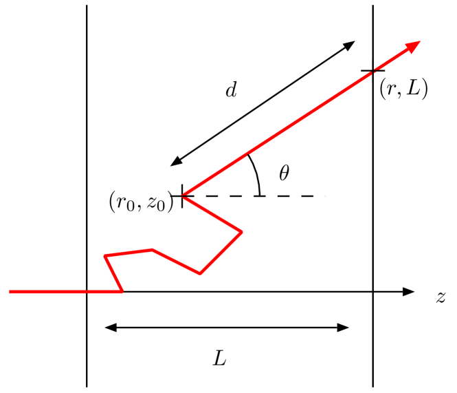
Figure 1: Notations used in a slab geometry to derive the radial dependance of the transmitted flux in the case of Lévy flights.

II.3 Long time behavior and Lévy flights

A Lévy flights signature can also be derived by looking at the dispersion relation of Eq. (21). To do so, we still consider a slab geometry of thickness $L$. If the system is illuminating from the left by a plane wave at normal incidence, the problem is invariant by rotation on the azimuthal angle $\varphi$ and by translation along $x$ and $y$. By integrating Eq. (14) over $\varphi$, we obtain

$$\left[\mu\frac{\partial}{\partial z}+\left(1+\frac{1}{\Gamma}\frac{\partial}{\partial t}\right)\mu_{\ell}\left(\delta\right)\right]I\left(\mu,z,\delta,t\right)\\ =\frac{\mu_{\ell}\left(\delta\right)}{2}\int p\left(\delta^{\prime}\right)I\left(\mu^{\prime},z,\delta^{\prime},t\right)\mathrm{d}\mu^{\prime}\mathrm{d}\delta^{\prime}.$$ (21)

We now perform a modal expansion of the specific intensity by taking its spatial Fourier transform combined with temporal eigenmodes Case and Zweifel (1967); Pierrat et al. (2006, 2009)) which leads to

$$I\left(\mu,z,\delta,t\right)=g_{ks}\left(\mu,\delta\right)\exp\left[ikz+s\left(k\right)t\right].$$ (22)

$g_{ks}$ can be interpreted as the eigenvector associated to the eigenvalue $s\left(k\right)$. Injecting this expression into Eq. (21) and defining a renormalized eigenvector by $G_{ks}\left(\mu,\delta\right)=p\left(\delta\right)g_{ks}\left(\mu,\delta\right)$, we obtain the dispersion relation of the transport equation given by

$$\int\frac{\mu_{\ell}\left(\delta\right)p\left(\delta\right)}{k}\arctan\left[\frac{k}{\left(1+s/\Gamma\right)\mu_{\ell}\left(\delta\right)}\right]\mathrm{d}\delta=1.$$ (23)

To obtain an explicit relation on $s$, we define $K=k/\left(1+s/\Gamma\right)$. The predominant spatial mode is such that $k=\pi/L$ Pierrat et al. (2006) where $L$ is the thickness of the slab. This implies that when $L\to\infty$, $k\to 0$ and $s\to 0$. This leads to $K\approx k$ and finally we obtain

$$\frac{s}{\Gamma}\approx\int_{-\infty}^{+\infty}\frac{\mu_{\ell}\left(\delta\right)p\left(\delta\right)}{k}\arctan\left[\frac{k}{\mu_{\ell}\left(\delta\right)}\right]\mathrm{d}\delta-1$$ (24)

when $k\to 0$. This equation gives the temporal decay rate of the transmitted flux for long times and as a function of the system size:

$$T_{\textrm{diff}}\left(t\right)\propto\exp\left[s\left(\frac{\pi}{L}\right)t\right].$$ (25)

This behavior could be observed in time resolved experiments which has already been done for quenched systems Savo et al. (2014). By taking the limit $k\to 0$ (large system sizes), we find $s\propto k^{\alpha}$ with $\alpha=1$ leading to an anomalous diffusion equation with a spatial derivative $\Delta^{\alpha/2}$ which confirms again the presence of Lévy flights Metzler et al. (1999).

Note that a link can be made easily between $s\left(k\right)$ and the step-size distribution $P\left(x\right)$. We find

$$\frac{s\left(k\right)}{\Gamma}=\int_{0}^{+\infty}\frac{\sin\left(kx\right)}{kx}P\left(x\right)\mathrm{d}x-1.$$ (26)

This expression shows that $ks$ is given by the Fourier transform of $P/x$ which implies that if $P\left(x\right)\propto x^{-\alpha-1}$ when $x\to\infty$ then $s\left(k\right)\propto k^{\alpha}$ when $k\to 0$.

II.4 Standard diffusion radial profiles

In II.2 the focus was on the asymptotic of the spatial distributions for Lévy flights. This asymptotic gives its characteristic signature. We found that the single-step fundamental Lévy $\alpha$ parameter [$P\left(x\right)\propto 1/x^{\alpha+1}$] survives in the multiple-step regime for a slab geometry in the form of a power law in the radial transmission profile [$T_{\textrm{diff}}(r)\propto r^{-3-\alpha}=1/r^{4}$]. Our main goal is to characterize unambiguously the Lévy regime, emphasising its qualitative difference from standard diffusion. We therefore tried to address the following question: what is the asymptotic in the multiple scattering regime in the spatial radial profile for standard diffusion? Is it exponential (possibly mimicking a single step step-size distribution); or alternatively, is it Gaussian (mimicking the Gaussian propagator in infinite media)? In trying to address this question we derived an analytical representation of the radial profiles in the slab for both transmission and reflection. This indeed gives a quasi-exponential asymptotic for standard diffusion, thus emphasizing an important physical insight. The qualitative nature of the single-step distribution still survives in the multi scattering regime: a Lévy signature can be inferred from a power law in the radial profile and a exponential radial dependence is the asymptotic signature of standard diffusion. The radial profiles in an infinite slab, for isotropic scattering and no absorption can be represented as:

$$R_{\textrm{diff}}\left(r\right)=\, \frac{\pi}{4}\left(\frac{1}{L_{e}}\right)^{2}i\left\{\sum_{n=1}^{+\infty}n\,\cos\left(n\pi\frac{z_{e}}{L_{e}}\right)\right.$$

$$\times\left.\vphantom{\sum_{n=1}^{+\infty}}\sin\left(n\pi\frac{\ell^{*}+z_{e}}{L_{e}}\right)\operatorname{H}_{0}^{\left(1\right)}\left(in\pi\frac{r}{L_{e}}\right)\right\},$$ (27)

$$T_{\textrm{diff}}\left(r\right)=\, \frac{\pi}{4}\left(\frac{1}{L_{e}}\right)^{2}i\left\{\sum_{n=1}^{+\infty}\left(-1\right)^{n+1}n\,\cos\left(n\pi\frac{z_{e}}{L_{e}}\right)\right.$$

$$\times\left.\vphantom{\sum_{n=1}^{+\infty}}\sin\left(n\pi\frac{\ell^{*}+z_{e}}{L_{e}}\right)\operatorname{H}_{0}^{\left(1\right)}\left(in\pi\frac{r}{L_{e}}\right)\right\},$$ (28)

where $L$ is the slab width, $\ell^{*}$ the transport mean-free path, and $L_{e}=L+2z_{e}$ an effective width, with $z_{e}$ an extrapolation length added to take into account the boundary conditions. $R_{\textrm{diff}}\left(r\right)$ and $T_{\textrm{diff}}\left(r\right)$ are the radial profiles in reflection and transmission. For details of the derivation, see appendix V.2.

The $\operatorname{H}_{n}^{\left(1\right)}$ are the Hankel $\operatorname{H}$ functions (Bessel functions of the third kind). Two properties of the Hankel functions are important for this work: their divergence at the origin and their asymptotic behaviour. We checked and, although each term in the previous series diverges by itself, the series is indeed convergent at the origin (details are given in the appendix V.2). More important is the asymptotic behavior. The asymptotic valid for large distances from the center (please remember that it is exactly this asymptotic behaviour that we sough) is easily obtained. The asymptotic for each term is Duffy (2001):

$$i\,\operatorname{H}_{0}^{\left(1\right)}\left(in\pi\frac{r}{L_{e}}\right)\sim\frac{1}{\pi}\,\sqrt{\frac{2L_{e}}{n}}\,r^{-1/2}\,\exp\left(-n\pi\frac{r}{L_{e}}\right).$$ (29)

For large distances, only the first term of the series survives and the asymptotic is approximately exponential [see Fig. 2(a)]. What emerges is an approximate exponential asymptotic for both the transmitted and reflected radial profiles. This quasi-exponential asymptotic can be interpreted as the signature of standard diffusion in the slab. This dependence is present in the analytical solution of the diffusion equation, as well as in the solution of the radiative transfer equation, not restricted to the diffusion approximation Liemert and Kienle (2012); Machida et al. (2010). Although the exponential asymptotic is only approximate, the $r^{-1/2}$ dependence is weak and in all practical situations a log-lin plot gives an easy graphical criteria to identify a diffusion-like asymptotic [see Fig. 2].

We checked that the sum of the overall reflection and transmission intensities, obtained by integrating over angle from Eqs. (27) and (28), is one. This is of course the expected result based on physical grounds: since absorption was not considered, this trivially expresses energy conservation.

Fig. 2 shows fits of the transmitted radial profile with the analytical model of Eq. (28), for both an experimental result (milk) as well as a Monte Carlo simulation. The fits with the diffusion model are very good (for the Monte Carlo, the fit is perfect, better than real life) and the agreement between the known slab width and the one recovered by fit is also very good: for milk, experimental $L=$16\pm 1\text{\,}\mathrm{mm}$$, by fit $L=$14.82\pm 0.05\text{\,}\mathrm{mm}$$; for Monte Carlo (with input parameters corresponding to the fitted ones, obtained from milk), one recovers by fit $L=$14.7\pm 3.5\text{\,}\mathrm{mm}$$. Part (a) puts in evidence the quasi-asymptotic regime and further illustrates the relative contribution of the first term in the series, the one giving the quasi-asymptotic, to the overall profile. Part (b) shows Monte Carlo data, also fitted with a simple Gaussian and a Power Law model. We use the Monte Carlo data to illustrate the inability of the Gaussian to adequately describe the data (also true for the experimental data). Fig. 2 is important since it shows perfect agreement with the diffusion prediction of Eq. (28), but also because it shows that the difference of a Gaussian to the analytical model is accessible in an actual experiment (our experimental setup easily access two to four orders of magnitude; the standard practice of plotting the profile in lin scale makes the disagreement with the Gaussian much less evident). It is also operational important since it dismiss any possible artifacts in the Monte Carlo general scheme (the general framework in which the Monte carlo of the Lévy flight, a far from trivial code, is constructed). And illustrates a simple graphical procedure to diagnose the qualitative signature of the data: a log-lin plot will signal diffusion, a log-log plot a power law (see Fig. 5, below).

In Fig. 2, the confidence interval for the fitted values of the mean transport length in very large. This finding was the motivation to make the Monte Carlo simulation using as input parameters the ones obtained from the fit of the milk data: we wanted to test the ability to recover meaningful values for the transport length. Although the agreement for $\ell^{*}$ between input and recovered by fit is satisfactory only when considering the corresponding confidence intervals, we found that in this well developed diffusion regime ($L/\ell^{*}=274$, for milk), Eq. (28) is very insensitive to the actual $\ell^{*}$ value. Therefore, in this regime, the transmitted profile is not the best observable to access meaningfully $\ell^{*}$ (tests not shown). This is the reason of a very broad confidence interval for the $\ell^{*}$ values of course. Additional technicalities of the fitting algorithm and limitations are given in appendix V.2.

The quality of the fit and the good agreement of the Monte Carlo data and the diffusion model illustrate that, at least for aspect ratios not smaller than the ones used in this work (for milk the ratio of slab width to diameter is roughly $10$), the diffusion model assuming an infinite slab is an adequate description of an actual experiment (please remember that both analytical model and Monte Carlo correspond to an infinite slab; actual experiment is always finite).

Figure 2: (Color online) Transmission profiles (experimental, with milk, and for a Monte Carlo simulation) and corresponding fits with an analytical model for diffusion, Eq. (28). (a) Experimental transmission profile ($\ell^{*}=$0.05\pm 1.5\text{\,}\mathrm{mm}$$, $L=$14.82\pm 0.05\text{\,}\mathrm{mm}$$). Also shown is the contribution of a single term, the first and slowest decaying of the series, the one responsible for the quasi-exponential asymptotic. (b) Monte Carlo (input parameters from the fit of the milk) for an infinite slab, fitted with the analytical model Eq. (28) (three fitting parameters: width, transport mean-free path and scale; $\ell^{*}=$0.09\pm 2.5\text{\,}\mathrm{mm}$$, $L=$14.7\pm 3.5\text{\,}\mathrm{mm}$$), with a Gaussian (two parameters: width and scale) and with a power law asymptotic law (two parameters: power law parameter and scale, plus a cut-off distance; here $20\text{\,}\mathrm{mm}$). The diffusion model is indistinguishable from the Monte Carlo data (even in a log scale spanning four orders of magnitude). The Gaussian and the power law are inadequate.

An important physical insight can be stressed at this point. Altough the actual details of standard and anomalous diffusion can be quite involved, their microscopic physical signature survives in the asymptotics of steady state in a strongly multiple scattering regime: standard diffusion with an exponential single step distribution gives rise to asymptoticaly exponential spatial profiles (and not to Gaussian profiles, as one might guess from the Gaussian propagator in infinite media) while a single step power law Lévy will reveal itself as a power law in the multiple step spatial profile. This insight is important since the fundamental nature of diffusion can be investigated in multiple scattering conditions, usually much easier to access than the corresponding single scattering counterparts.

III Experiment

III.1 Setup description

Experimentally, microscopic measurements of the step-size distribution have already been realized Mercadier et al. (2009) showing the existence of Lévy flights of light in hot atomic vapors. In this article, we focus on the macroscopic evidence of Lévy flights by recovering the Lévy parameter $\alpha$ using a stationary experiment under multiple scattering conditions. Our experiment is really close to ideal Gedanken experiment. We consider a flat cell (Petri dish shape made of pirex) of diameter $10\text{\,}\mathrm{cm}$, external thickness $11\text{\,}\mathrm{mm}$ and internal thickness $L=$5\text{\,}\mathrm{mm}$$. It contains a natural mixture of 85 and 87 rubidium vapor. This cell is illuminated by a distributed feedback (DFB) laser whose spectral width is on the order of $2\text{\,}\mathrm{M}\mathrm{H}\mathrm{z}$ and the maximum of power before cell can reach several milliwatts. Not to saturate atoms and CCD camera we use only few dozen microwatts after several attenuators. One part of the incident laser is used for rubidium spectroscopy and for locking on the $F=2\to F^{\prime}=2\relbar F^{\prime}=4$ crossover of the D2 line of ⁸⁵Rb. The laser has a piedestal $40\text{\,}\mathrm{d}\mathrm{B}$ below the laser peak but with some nanometers of width. This piedestal can be a problem since, even if it is out of resonance of rubidium and does not scatter on rubidium, a part scatters on the sides of cell. The main part of the laser beam is injected in a monomode fiber whose output shines the center of the cell. The laser is collimated with a waist of $w\approx$1.3\text{\,}\mathrm{mm}$$. The cell is placed on an oven whose temperature can be controlled homogeneously between $40\text{\,}\mathrm{\SIUnitSymbolCelsius}$ to $170\text{\,}\mathrm{\SIUnitSymbolCelsius}$, therefore tuning the density of atoms $\rho$ between around $6\times\power{10}{15}\text{\,}\mathrm{a}\mathrm{t}\mathrm{/}\mathrm{m}^{3}$ and $2\times\power{10}{20}\text{\,}\mathrm{a}\mathrm{t}\mathrm{/}\mathrm{m}^{3}$. The laser source is one meter far from oven to avoid temperature control problems.

Experimentally, the optical thickness $b\left(\omega\right)$ and the extinction coefficient $\mu_{\ell}\left(\omega\right)$ are not the most convenient quantities to characterize the optical response of the cell in particular because of their dependences on the frequency. We prefer to use in the following the opacity $O$ and the scattering cross section $\sigma_{T}\left(\omega\right)$. The opacity is defined by

$$O=\frac{L}{\ell_{0}}.$$ (30)

As $\ell_{0}$ depends on the density $\rho$, it is possible to tune in a well controlled manner the opacity by just changing the temperature. In particular, the range of temperature considered in the experiment corresponds to a change in opacity $O$ from $\power{10}{2}$ to $\power{10}{5}$. The opacity is thus a good indicator of an effective cell thickness and the scaling laws for $O$ and $L$ are identical. Using this definition, the optical thickness becomes

$$b\left(\omega\right)=\frac{L}{\ell\left(\omega\right)}=O\frac{\ell_{0}}{\ell\left(\omega\right)}=O\frac{\sigma_{T}\left(\omega\right)}{\sigma_{0}}$$ (31)

where $\sigma_{0}$ is the scattering cross section of a pinned atom at resonance. $\sigma_{T}\left(\omega\right)$ is given by

$$\sigma_{T}\left(\omega\right)=\int\sigma\left(\omega-\boldsymbol{\mathbf{k}}\cdot\boldsymbol{\mathbf{v}}\right)g\left(\boldsymbol{\mathbf{v}}\right)\mathrm{d}\boldsymbol{\mathbf{v}}$$ (32)

with the scattering cross section for atoms at rest given by

$$\sigma\left(\omega\right)=\sum_{i}R_{i}\pi_{i}\frac{\sigma_{0}}{1+4\delta_{i}^{2}},$$ (33)

$R_{i}$ being the branching ratios of each hyperfine line $i$ of the D2 line of ⁸⁵Rb and ⁸⁷Rb. The detunings are given by $\delta_{i}=\left(\omega-\omega_{0,i}\right)/\Gamma$ where $\omega_{0,i}$ are resonance frequencies and $\Gamma$ the linewidth.

III.2 Ballistic transmission measurement

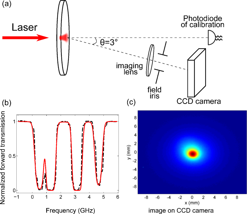
Figure 3: (Color online) (a) Experimental setup: A laser beam is incident on a flat cylindrical cell filled with a rubidium vapor. The transmitted ballistic light spectrum is measured via a photodiode aligned with the laser beam. The scattered light coming out of the slab is imaged on the CCD camera misaligned by an angle of $3\text{\,}\mathrm{\SIUnitSymbolDegree}$ with the laser. (b) Signal of the photodiode: The transmission of the laser scanned in frequency throughout the rubidium cell shows the D2 hyperfine absorption of ⁸⁵Rb and ⁸⁷Rb. An ab-initio fit of this signal is used to deduce the opacity $O$. Even if the system is strongly scattering, a coherent transmission measurement can still be done especially out of resonance where the optical thickness is weaker. (c) Image of the radial profile observed on the CCD camera.

Experimentally, the opacity $O$ is estimated by measuring the coherent transmission $T_{\textrm{coh}}\left(\omega\right)$ of a laser beam through the cell using a photodiode [see Fig. 3 (a)]. It is given by

$$T_{\textrm{coh}}\left(\omega\right)=\exp\left[-\rho L\sigma_{T}\left(\omega\right)\right]=\exp\left[-O\frac{\sigma_{T}\left(\omega\right)}{\sigma_{0}}\right].$$ (34)

The incident frequency is tuned to scan all D2 lines of two rubidium isotopes [see Fig. 3 (b)]. In our range of temperature, the opacity scales as $O\sim 200\log\left(T\right)$ which ensures the multiple scattering regime. The spectral broadening is proportional to the square root of the temperature while the vapor pressure depends exponentially on the temperature ensuring that the Doppler effect is almost not affected by the temperature.

III.3 Diffuse transmission measurement

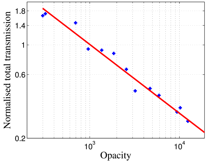
Figure 4: (Color online) Total diffuse transission in log scale as a function of the opacity. Blue crosses: Experimental data. Each point corresponds to the sum of all pixels of a CCD image for a given opacity. Black solid line: fit of the experimental data. The power law obtained is $T_{\textrm{diff}}\propto O^{-0.516\pm 0.024}$.

We now turn into the stationary diffuse transmission measurement. For long term stability and an absolute frequency reference, we lock the laser on the $F=2\to F^{\prime}=2\relbar F^{\prime}=4$ crossover of the D2 line of ⁸⁵Rb.

Due to a residual background of amplified spontaneous emission (ASE) of our DFB laser, scattering of this spectrally broad pedestal on the facets of our rubidium cell give rise to an additional offset signal. As we focus on the power law tails in the image, the center of the image (where such background scattering is present) does not affect the result of our analysis. We however noted that when using an imaging system with a $25\text{\,}\mathrm{mm}$ diameter lens, the depth of field (DOF) was small enough to blurr the image of the scattered component of the ASE on the input facet of our cell. Indeed, a small DOF results in a diffractive type power tail in the detected image of light scattered from an object beyond the DOF. Even though the power in the pedestal of our DFB laser only represents about $0.4\text{\,}\%$ of the power of the laser, this can limit the possibility to detect the relevant power law tails under consideration. This effect would be a crucial limititation to the light scattered by the atoms at large distances. One solution would be to use a laser with a reduced ASE background. In our setup, we solved this problem by decreasing the diameter of an iris placed in front of the imaging lens from $25\text{\,}\mathrm{mm}$ to $10\text{\,}\mathrm{mm}$. We thus deliberately increased the DOF beyond the length of our rubidium cell. Light scattered on the windows of both input and output facets of the cell are thus only visible at the center of the image at the CCD, not contributing to the wings of the radial profile, where we extract the Lévy flight information from the light scattered by the atoms. We have checked that using an iris diameter of $10\text{\,}\mathrm{mm}$, the radial profile measured by the CCD camera, with the laser tuned out of the atomic resonance line, decreases by more than 4 orders of magnitude at only $2\text{\,}\mathrm{mm}$ whereas with a fully open iris, the same reduction is obly obtained at $10\text{\,}\mathrm{mm}$. As the image of the relevant output spot is small compare to CCD camera, we use the pixels in peripheria to define the background signal to subtract. Increased signal to noise ratio is obtained by averaging with an interpolation method over $36$ cuts across the center of the image (each rotated by $10\text{\,}\mathrm{\SIUnitSymbolDegree}$). Subsequent smoothing of the data further improves the signal to noise ratio shown in Fig. 5.

In Fig. 4 we plot the total transmission incoming on all pixels of the CCD camera as a function of the opacity. This does not correspond exactly to the total transmitted energy outgoing the system because of the small numerical aperture considered. Nevertheless, we have checked numerically using the Monte Carlo simulation that this does not affect the scaling law. We clearly see that the total transmission $T_{\textrm{diff}}$ does not scale as Ohm’s law prediction (i.e. $T_{\textrm{diff}}\propto O^{-1}$) but has a superdiffusive behavior (i.e. $T_{\textrm{diff}}\propto O^{-0.516}$), in excellent agreement with the prediction at large opacities $T_{\textrm{diff}}\propto O^{-\alpha/2}$ for $\alpha\approx 1$ Davis and Marshak (1997); Barthelemy et al. (2008). Considering the single step size distribution measured in Mercadier et al. (2009) this exponent is in excellent agreement with the expectation for the total diffuse transmission for a Lévy walk of independent steps and different from random walk in quenched disorder Groth et al. (2012).

Exploiting the excellent signal to noise ratio of our angular averaged CCD images, we also plot the radial profile of the transmitted intensity $T_{\textrm{diff}}(r)$ in linear [see Fig. 5 (a)] and logarithmic [see Fig. 5 (b)] scales, highlightening the large dynamic range of our signal. We clearly see that the general shape is far from a gaussian profile. The tail clearly exhibits a power law: $T_{\textrm{diff}}(r)\propto r^{-4.03\pm 0.15}$, as predicted by Eq. (20) for $\alpha=1.01\pm 0.04$. Moreover, this asymptotic behavior is valid for a wide range of opacities as shown on Fig. 5 (c). We note that for increasing opacity, the total relevant signal is reduced [see Fig. 4] and the relative importance of amplified spontaneous emission pedestal increases, requiring thus to adapt the range of radial distances where a reasonable fit can be obtained. Finally, we stress that the scaling laws in the tail of $T_{\textrm{diff}}(r)$ can be obtained from a single image on the CCD, giving access to Lévy parameter with a single snapshot whose duration is $2\text{\,}\mathrm{ms}$. This has to be compared to previous studies where the Lévy parameter were extracted in $30\text{\,}\mathrm{h}$ Mercadier et al. (2013). Also, with only one snapshot, the vertical dynamics is more than four orders of magnitude and allow a good fit. Furthermore, this single image under multiple scattering condition allows to make use of these scaling laws in different experimental conditions, in laboratory environment or in astrophysical systems.

One interesting point concerning the radial profile is the behavior at small distances $r$. In Lévy glasses Barthelemy et al. (2008), a pronounced cusp is observed close to $r=0$ which is not the case neither in our experiment nor in simulations. There are several fundamental differences between Lévy glasses and hot atomic vapors illuminated by a monochromatic laser beam. For Lévy glasses, when light enters the system, the step-size distribution is already a power law with an exponent $\alpha<2$ leading to superdiffusion. In our hot vapor experiment in contrast, the correct step-size distribution for photons at the laser frequency is an exponential function $\mu_{\ell}\left(\delta_{0}\right)\exp\left[-\mu_{\ell}\left(\delta_{0}\right)x\right]$, different from the power law step-size distribution after one scattering event, where the frequency is already redistributed. We have checked numerically that if a broadband excitation were used to illuminate the hot atomic vapor cell, a sharp cusp around the center of the transmitted light path is recovered.

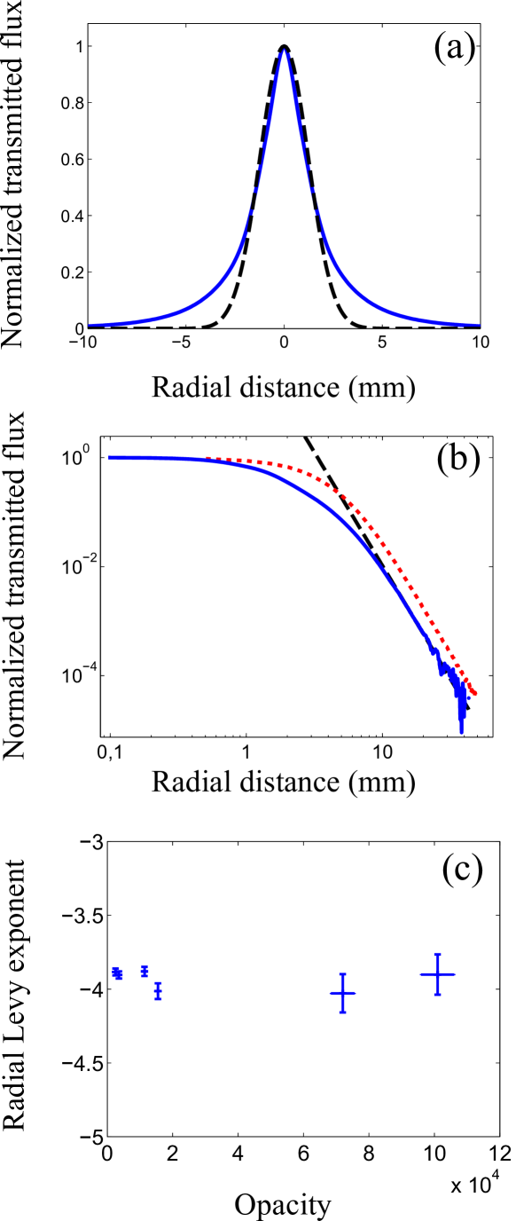
Figure 5: (Color online) (a) Blue solid line: Experimental radial profile (in linear scale) of the scattered light transmitted through the cell. Black dashed line: Gaussian profile with the same width at half maximum as the experimental profile. (b) Blue solid line: Experimental radial profile (in log scale) of the scattered light transmitted through the cell. Dotted red line: Numerical prediction from a Monte Carlo simulation of the transport equation. Black dashed line: fit of the experimental data in the range $[1.1,2.1]\text{\,}\mathrm{cm}$. The power law obtained is $T_{\textrm{diff}}(r)\propto r^{-4.03\pm 0.15}$. The temperature is $T=$114\text{\,}\mathrm{\SIUnitSymbolCelsius}$$ corresponding to an opacity of $O=$1.15\text{\,}\times${\power{10}{4}}$ and an optical thickness of $b=540$. (c) Power law exponent of the radial profile tail of the transmitted intensity $T_{\textrm{diff}}(r)$ as a function of the opacity $O$ tuned by varying the temperature. This exponent is close to $-4$ for a wide range of opacity showing the robustness of the Lévy character of the system. Vertical error bars correspond to standard deviation of the fit to extract the power law of $T_{\textrm{diff}}(r)$. Error bars increase for large opacities due to the decrease of the relevant signal.

IV Conclusion

In summary, we have shown theoretical, numerical and experimental results confirming Lévy flights of photons in hot vapor under multiple scattering condition with annealed disorder. Lévy flights in our system appear due to the interplay between the high quality factor of atomic resonances and large Doppler broadening. The scaling laws obtained for the total diffuse transmission $T_{\textrm{diff}}$ and intensity profile $T_{\textrm{diff}}(r)$ suggests that other spectral broadenings such as collisions with a buffer gas could allow to enhance or control Lévy flights and will be accessible in realistic experimental conditions. This work opens also new perspectives to look for evidence of Lévy flight in astrophysical systems or for quantitative studies of the limits of validity of the complete frequency redistribution in hot vapors.

V Appendices

V.1 Monte Carlo scheme

The exact numerical resolution of Eq. (14) is possible using a Monte Carlo scheme. As a Monte Carlo algorithm is designed to evaluate numerically complex integrals, a new form of the integro-differential transport equation has to be written. First, we take the Fourier transform of Eq. (14) with respect to the space and time variables which gives

$$\left[i\boldsymbol{\mathbf{u}}\cdot\boldsymbol{\mathbf{q}}+\left(1-\frac{i\Omega}{\Gamma}\right)\mu_{\ell}\left(\delta\right)\right]I\left(\boldsymbol{\mathbf{u}},\boldsymbol{\mathbf{q}},\delta,\Omega\right)\\ =\frac{\mu_{\ell}\left(\delta\right)}{4\pi}\int p\left(\delta,\delta^{\prime},\boldsymbol{\mathbf{u}},\boldsymbol{\mathbf{u}}^{\prime}\right)I\left(\boldsymbol{\mathbf{u}}^{\prime},\boldsymbol{\mathbf{q}},\delta^{\prime},\Omega\right)\mathrm{d}\boldsymbol{\mathbf{u}}^{\prime}\mathrm{d}\delta^{\prime}.$$ (35)

Using this expression, we can easily isolate the Fourier transform of the specific intensity $I\left(\boldsymbol{\mathbf{u}},\boldsymbol{\mathbf{q}},\delta,\Omega\right)$. Noticing that

$$\left[i\boldsymbol{\mathbf{u}}\cdot\boldsymbol{\mathbf{q}}+\left(1-\frac{i\Omega}{\Gamma}\right)\mu_{\ell}\left(\delta\right)\right]^{-1}\\ =\int_{0}^{\infty}\exp\left[-\left\{i\boldsymbol{\mathbf{u}}\cdot\boldsymbol{\mathbf{q}}+\left(1-\frac{i\Omega}{\Gamma}\right)\mu_{\ell}\left(\delta\right)\right\}s\right]\mathrm{d}s$$ (36)

we obtain

$$I\left(\boldsymbol{\mathbf{u}},\boldsymbol{\mathbf{q}},\delta,\Omega\right)=\frac{\mu_{\ell}\left(\delta\right)}{4\pi}\\ \times\int_{s=0}^{\infty}\exp\left[-\left\{i\boldsymbol{\mathbf{u}}\cdot\boldsymbol{\mathbf{q}}+\left(1-\frac{i\Omega}{\Gamma}\right)\mu_{\ell}\left(\delta\right)\right\}s\right]\\ \times\int p\left(\delta,\delta^{\prime},\boldsymbol{\mathbf{u}},\boldsymbol{\mathbf{u}}^{\prime}\right)I\left(\boldsymbol{\mathbf{u}}^{\prime},\boldsymbol{\mathbf{q}},\delta^{\prime},\Omega\right)\mathrm{d}\boldsymbol{\mathbf{u}}^{\prime}\mathrm{d}\delta^{\prime}\mathrm{d}s.$$ (37)

Finally, by taking the inverse Fourier transform of the last expression, we find

$$I\left(\boldsymbol{\mathbf{u}},\boldsymbol{\mathbf{r}},\delta,t\right)=\int_{s=0}^{\infty}\mu_{\ell}\left(\delta\right)\exp\left[-\mu_{\ell}\left(\delta\right)s\right]\\ \times\int\frac{p\left(\delta,\delta^{\prime},\boldsymbol{\mathbf{u}},\boldsymbol{\mathbf{u}}^{\prime}\right)}{4\pi}I\left(\boldsymbol{\mathbf{u}}^{\prime},\boldsymbol{\mathbf{r}}-s\boldsymbol{\mathbf{u}},\delta^{\prime},t-\frac{\mu_{\ell}\left(\delta\right)s}{\Gamma}\right)\mathrm{d}\boldsymbol{\mathbf{u}}^{\prime}\mathrm{d}\delta^{\prime}\mathrm{d}s.$$ (38)

This form is very convenient to derive the Monte Carlo algorithm dedicated to the resolution of Eq. (14). In particular, it shows that the probability density to perform a step of length $s$ between two scattering events is given by $\mu_{\ell}\left(\delta\right)\exp\left[-\mu_{\ell}\left(\delta\right)s\right]$ and the probability densities to be scattered in a direction $\boldsymbol{\mathbf{u}}$ from a direction $\boldsymbol{\mathbf{u}}^{\prime}$ and at a frequency $\delta$ from a frequency $\delta^{\prime}$ are respectively given by $1/\left(4\pi\right)$ and $p\left(\delta,\delta^{\prime},\boldsymbol{\mathbf{u}},\boldsymbol{\mathbf{u}}^{\prime}\right)$. As the probability densities are known analytically, no truncation is performed and the method of resolution is exact, the numerical error being given by the number of energy packets sent into the system.

V.2 Standard diffusion radial profiles

This appendix is dedicated to the technicalities of the derivation of the asymptotic behavior of the radial profile of the transmitted or reflected intensity in the case of classical diffusion. The diffusion equation is solved for an infinite slab, in steady state, using two canonical approximations: the source term is substituted for a unit delta production (at a transport mean-free path $\ell^{*}$ from left side; excitation is assumed to impinge from left) and Dirichlet boundary conditions, defined at a so called extrapolation length ($z_{e}$; the effective width is $L_{e}=L+2z_{e}$, with $L$ the slab width) Zhu et al. (1991). The problem to solve is $-D\nabla^{2}I\left(\boldsymbol{\mathbf{r}}\right)=\delta\left(\boldsymbol{\mathbf{r}}\right)$, with $I\left(z=0\right)=I\left(z=L_{e}\right)=0$ (the origin of the $z$ coordinate makes the application of the theory of Green functions –fundamental Green function and multiple image series or, alternatively, the expansion in eigenfunctions– the simplest possible). Two further quantities are defined: the flux $\Phi\equiv-D\partial I\left(\boldsymbol{\mathbf{r}}\right)/\partial z$ and the radial profiles, in reflection and transmission, $\left\{R_{\textrm{diff}}\left(r\right)=-\Phi\left(z=z_{e}\right),T_{\textrm{diff}}\left(r\right)=\Phi\left(z=L+z_{e}\right)\right\}$, here assumed with axial symmetry (experimental case). It is assumed no absorption. We only use the transmitted profile, but quote also the one in reflection, for reference.

The solution in Fourier space is known Barthelemy (2009) and is given by

$$R_{\textrm{diff}}\left(q_{\bot}\right) =\frac{1}{2\pi}\frac{\cosh\left(q_{\bot}z_{e}\right)\sinh\left(q_{\bot}\left(L_{e}-\left(\ell+z_{e}\right)\right)\right)}{\sinh\left(q_{\bot}L_{e}\right)},$$ (39)

$$T_{\textrm{diff}}\left(q_{\bot}\right) =\frac{1}{2\pi}\frac{\cosh\left(q_{\bot}z_{e}\right)i\sinh\left(q_{\bot}\left(\ell+z_{e}\right)\right)}{\sinh\left(q_{\bot}L_{e}\right)},$$ (40)

where $q_{\bot}$ is the Fourier conjugate of the radial distance (the $2\pi$ is dependent on Fourier notation choice). The solution in physical space is obtained by performing the inverse Fourier transform, as usual. Care must be exercised in two points: it’s a 2D Fourier inverse transform and the implementation of the residues theorem must take into account the asymptotic nontrivial behavior of the Bessel function. The final solution in physical space is given by Eqs. (27) and (28).

Its derivation used the facts Baddour (2011); Abramowitz and Stegun (1972):

1. the 2D Fourier transforms of axial symmetric functions are the Hankel transforms of zero order;

2. the Bessel function can be written as

   $$\operatorname{J}_{n}\left(z\right)=\frac{1}{2}\left[\operatorname{H}_{n}^{\left(1\right)}\left(z\right)+\operatorname{H}_{n}^{\left(2\right)}\left(z\right)\right];$$ (41)

3. the special Hankel functions asymptotics are
   $\left\{\operatorname{H}_{n}^{\left(1\right)}\left(z\right)\rightarrow 0,\,\left|z\right|\rightarrow\infty\,\&\,0<\arg\left(z\right)<\pi,\right.$ $\left.\operatorname{H}_{n}^{\left(2\right)}\left(z\right)\rightarrow 0,\,\left|z\right|\rightarrow\infty\,\&\,-\pi<\arg\left(z\right)<0\right\}$.

V.3 Fitting details

This appendix is dedicated to several aspects of the various fitting procedures, used in the main body of the paper.

The correct use of the analytical representations of the radial profiles in Eqs. (27) and (28) requires special care near the origin. The Hankel functions in these equations diverge at the origin. We do not have an analytical proof of the series convergence. However, we made a detailed study of the convergence speed, near the origin and found empirical evidence of the convergence: in all cases, using a sufficiently high number of terms, we verified the convergence of the series. We nevertheless emphasize that the convergence is very slow: by values of the argument of the order of $\power{10}{-5}$, we needed about $40000$ terms to warrant convergence. All the fits in this work used a fixed number of terms in the series ($2500$, a conservative estimate, based in the smallest distance we used).

The effective use of Eqs. (27) and (28) in fitting routines requires care in at least two details. The first was already mentioned: check convergence, at the smallest distance. The second is connected with the limitations embedded by the physics. If $\ell^{*}\ll L$, then $L_{e}\sim L$ and the exponential asymptotic does not depend upon the transport mean-free path. In fact, the normalized transmitted profile is effectively constant in this well developed diffusion regime, thus reducing the ability to recover meaningfully parameters by fitting Eqs. (28) to experimental data. This of course is what is expected from simple physical arguments. In these cases, a better approach is to devise an experimental setup in which both reflection and transmission profiles are accessible at the same time. A global analysis will have $\ell^{*}$ sensible fitted from the central part of the reflection, and $L$ from the asymptotic of both reflection and transmission.

A detailed parameter space exploration of Eqs. (27) and (28), to judge whether one can expect artifacts, is not the focus of this work. However, we checked a posteriori and indeed, the transmission profile is quite insensitive to the actual value of the $\ell^{*}$ value, in the fits of Fig. 2. This can also be quantified in a computational linear algebra approach by the actual value of the condition number of the fitting matrix, the ratio of biggest to smallest eigenvalue of a decomposition of the Hessian matrix of the fit. In the fits of Fig. 2, the condition number is of the order of $\power{10}{-9}$. This is a very small value thus signaling instrinsic numerical limitations. Given all these arguments, the agreement between Monte Carlo input parameters $\ell^{*}=$0.05\text{\,}\mathrm{mm}$$, $L=$14.82\text{\,}\mathrm{mm}$$) and the ones recovered by fitting ($\ell^{*}=$0.09\pm 2.5\text{\,}\mathrm{mm}$$, $L=$14.7\pm 3.5\text{\,}\mathrm{mm}$$) is very good.

An important detail connected with the procedures used in this work for statistical inference should be highlighted. It is well known that fitting to a power law is notoriously difficult. This of course results from the fact that, in order to have meaningful fitted values of the power law exponent, one must include in the statistical inference values spanning several orders of magnitude (in principle, as many as possible). Two general procedures are then available: either data analyse binned of unbinned information. The unbinned information is preferable in theoretical grounds since the binning of data can make the estimators biased. The use of maximum likelihood estimators for unbinned data is far less prone to artefacts Golstein et al. (2004). This is the cause of the use of unbinned data in such classical works as Viswanathan et al. (1996); Edwards et al. (2007), where animal foraging movements are tracked. However, one of the strongest arguments of the experimental study we present in this work is the very high signal to noise ratio we are able to achieve by analysing CCD images. It is as if each individual photon corresponded to a single event, in animal tracking studies. We have in a single $2\text{\,}\mathrm{ms}$ snapshot probably more information than all the data collected thus far in all the animal tracking studies realized thus far by humankind. By using a CCD, the data is already recorded in a binned (in each pixel) format. And we obtain very high signal to noise ratios, spanning as much as four orders of magnitude in dynamical range. We do not have access to the unbinned data and can not check for artefacts the data analysis we used (we used Levenberg-Marquardt nonlinear least squares algotrithms, which are also unbiased maximum likelihood estimators, for a Gaussian distribution of the signal in each pixel of the camera), by comparing the results obtained for unbinned data analysis. We nevertheless made your best efforts to dismiss fitting artefacts: we fitted the data in Fig. 2 using nonlinear least squares, unweighted in linear scale as well as weighted (Poisson counting, weight due to change of independent variable into a logarithmic scale), using linear least squares in a log-log scale and also testing the sensitivity of the actual fitted parameters to the initial approximations. In all cases, the differences in the power law parameter was smaller than the confidence intervals we quote in this work.

References

- Sebbah (2001) P. Sebbah, Waves and Imaging through Complex Media (Kluwer Academic, Dordrecht, 2001).
- Anderson (1958) P. Anderson, Phys. Rev. 109, 1492 (1958).
- Thomas and Stamnes (1999) G. E. Thomas and K. Stamnes, Radiative Transfer in the Atmosphere and Ocean (University Press, Cambridge, 1999).
- Tuchin (1997) V. Tuchin, Physics - Uspekhi 40, 495 (1997).
- Klages et al. (2008) R. Klages, G. Radons, and I. M. Sokolov, eds., Anomalous Transport, Foundations and Applications (Wiley-VCH, 2008).
- Viswanathan et al. (1996) G. M. Viswanathan, V. Afanasyev, S. V. Buldyrev, E. J. Murphy, P. A. Prince, and H. E. Stanley, Nat. 427, 413 (1996).
- Edwards et al. (2007) A. M. Edwards, R. A. Philipps, N. W. Watkins, M. P. Freeman, E. J. Murphy, V. Afanasye, S. V. Buldyrev, M. G. E. da Luz, E. P. Raposo, H. E. Stanley, et al., Nat. 449, 1044 (2007).
- Brockmann et al. (2006) D. Brockmann, L. Hufnagel, and T. Geisel, Nat. 398, 462 (2006).
- González et al. (2008) M. C. González, C. A. Hidalgo, and A.-L. Barabási, Nat. 453, 779 (2008).
- Shlesinger et al. (1987) M. F. Shlesinger, B. J. West, and J. Klafter, Phys. Rev. Lett. 58, 1100 (1987).
- Corral (2006) Á. Corral, Phys. Rev. Lett. 97, 178501 (2006).
- Baiesi et al. (2006) M. Baiesi, M. Paczuski, and A. L. Stella, Phys. Rev. Lett. 96, 051103 (2006).
- Barthelemy et al. (2008) P. Barthelemy, J. Bertolotti, and D. S. Wiersma, Nature 453, 495 (2008).
- Bertolotti et al. (2010) J. Bertolotti, K. Vynck, L. Pattelli, P. Barthelemy, S. Lepri, and D. Wiersma, Avd. Func. Mat. 20, 965 (2010).
- Svensson et al. (2013) T. Svensson, K. Vynck, M. Grisi, R. Savo, M. Burresi, and D. S. Wiersma, Phys. Rev. E 87, 022120 (2013).
- Barthelemy et al. (2010) P. Barthelemy, J. Bertolotti, K. Vynck, S. Lepri, and D. Wiersma, Phys. Rev. E 82, 011101 (2010).
- Alves-Pereira et al. (2007) A. R. Alves-Pereira, E. J. Nunes-Pereira, J. M. G. Martinho, and M. N. Berberan-Santos, J. Chem. Phys. 126, 154505 (2007).
- Groth et al. (2012) C. W. Groth, A. R. Akhmerov, and C. W. J. Beenakker, Phys. Rev. E 85, 021138 (2012).
- Kenty (1932) C. Kenty, Phys. Rev. 42, 823 (1932).
- Pereira et al. (2004) E. Pereira, J. M. G. Martinho, and M. N. Berberan-Santos, Phys. Rev. Lett. 93, 120201 (2004).
- Svensson et al. (2014) T. Svensson, K. Vynck, E. Adolfsson, A. Farina, A. Pifferi, and D. S. Wiersma, Phys. Rev. E 89, 022141 (2014).
- Holstein (1947) T. Holstein, Phys. Rev. 72, 1212 (1947).
- Mercadier et al. (2009) N. Mercadier, W. Guerin, M. Chevrollier, and R. Kaiser, Nat. Phys. 5, 602 (2009).
- Pierrat et al. (2009) R. Pierrat, B. Grémaud, and D. Delande, Phys. Rev. A 80, 013831 (2009).
- Chandrasekhar (1950) S. Chandrasekhar, Radiative Transfer (Dover, New-York, 1950).
- Unno (1952) W. Unno, Publ. Astron. Soc. Jap. 3, 158 (1952).
- Davis and Marshak (1997) A. Davis and A. Marshak, Lévy kinetics in slab geometry: scaling of transmission probability,in Fractal Frontiers, Eds. M.M. Novak, T.G. Dewey, World Scientific (World Scientific, Singapore, 1997), p. 63.
- Case and Zweifel (1967) K. M. Case and P. F. Zweifel, Linear Transport Theory (Addison-Wiley, Reading, Massachusetts, 1967).
- Pierrat et al. (2006) R. Pierrat, J. J. Greffet, and R. Carminati, J. Opt. Soc. Am. A 23, 1106 (2006).
- Savo et al. (2014) R. Savo, M. Burresi, T. Svensson, K. Vynck, and D. S. Wiersma, arXiv p. 1312.5962 (2014).
- Metzler et al. (1999) R. Metzler, E. Barkai, and J. Klafter, Physica A: Statistical Mechanics and its Applications 266, 343 (1999), ISSN 0378-4371.
- Duffy (2001) D. Duffy, Green’s Function with Applications (CRC, 2001).
- Liemert and Kienle (2012) A. Liemert and A. Kienle, JOSA A 29, 1475 (2012).
- Machida et al. (2010) M. Machida, G. Panasyuk, J. Schotland, and V. Markel, J.Phys.A: Math.Theor. 43, 065402 (2010).
- Mercadier et al. (2013) N. Mercadier, M. Chevrollier, W. Guerin, and R. Kaiser, Phys. Rev. A 87, 063837 (2013).
- Zhu et al. (1991) J. Zhu, D. Pine, and D. Weitz, Phys. Rev. A 44, 3948 (1991).
- Barthelemy (2009) P. Barthelemy, Anomalous Transport of Light, Ph.D. Thesis (LENS, 2009).
- Baddour (2011) N. Baddour, AIP Advances 1, 022120 (2011).
- Abramowitz and Stegun (1972) M. Abramowitz and I. Stegun, Handbook of Mathematical Functions, 10th Printing (National Bureau of Standards, 1972).
- Golstein et al. (2004) M. L. Golstein, S. A. Morris, and G. G. Yen, Eur. Phys. J. B 41, 255 (2004).