Quantum atomic lithography via cross-cavity optical Stern-Gerlach Setup

Abstract

We present a fully quantum scheme to perform 2D atomic lithography based on a cross-cavity optical Stern-Gerlach setup: an array of two mutually orthogonal cavities crossed by an atomic beam perpendicular to their optical axes, which is made to interact with two identical modes. After deriving an analytical solution for the atomic momentum distribution, we introduce a protocol allowing us to control the atomic deflection by manipulating the amplitudes and phases of the cavity field states. Our quantum scheme provides subwavelength resolution in the nanometer scale for the microwaves regime.

At the beginning of the 1990s, the optical Stern-Gerlach (OSG) effect Sleator was explored in a number of studies HAS ; FH ; BB , with a view to extracting information about a cavity field state through its interaction with an atomic meter. Relying on the fact that the momentum distribution of scattered atoms follows the photon statistics of the field state, strategies have been devised to reconstruct the statistics HAS and even the full state of a cavity mode FH . These OSG strategies differ from other measurement devices in quantum optics, such as quantum nondemolition Brag and homodyne techniques VR , that have been extensively explored from the 1990s until now Exp . More recently, a cross-cavity OSG has been proposed —where a beam of atoms is made to cross two orthogonal cavities— to measure the location and center-of-mass wave-function of the atoms Zubairy ; ADK . Although the cross-cavity OSG has not yet been implemented experimentally, the cross-cavity setup has been built to test Lorentz invariance at the $10^{-17}$ level Peters .

In addition to the developments in probing atomic and cavity-field states, atomic lithography —where classical light is used to focus matter on the nanometer scale— has also witnessed considerable progress in recent decades Pfau . The atom-light interaction is manipulated to assemble structured array of atoms with potential applications to nanotechnology-related fields. Beyond the achievements in the growth of spatially periodic and quasi-periodic Kampen atomic patterns Pfau , recent works have explored the possibility of creating nonperiodic arrays by using complex optical fields 12-13 ; Saffman .

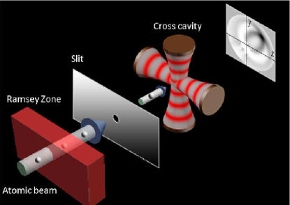
Figure 1: (color online). Sketch of the cross-cavity OSG.

In this paper, we present a scheme to realize two-dimensional (2D) quantum atomic lithography. In order to characterize it, we derive an analytical solution for the 2D OSG problem. We consider the cross-cavity OSG setup sketched in Fig. 1, where, before entering the cavities, the atoms are confined by a circular pinhole to a small region of space, centered around the superimposed nodes of the two cavity modes. Differently from the developments in Refs. Zubairy ; ADK , where dispersive atom-field interactions take place, we assume the two-level atoms to undergo simultaneous and resonant interactions with two identical modes, one from each cavity, thus being deflected in the plane defined by the two mutually perpendicular cavities’ optical axes. An appropriate ansatz on the spatial distribution of the atoms across the pinhole enables us to derive an analytical expression for the atomic momentum distribution after the atom-field interactions. Our protocol to generate 2D nonperiodic complex atomic patterns is based on a map that relates the transverse momentum acquired by the atoms to the previously prepared cavity-field state. Interestingly, we find that the (abstract) momentum-quadrature components of the field states are directly associated with the (real) atomic momentum components.

Before addressing the cross-cavity OSG, it is worth mentioning previous works in the Literature on quantized light lenses for atomic waves. We start with the proposals for focusing and deflecting an atomic beam through quantized field, which also addresse the process of creating regular structures with a period of atomic size Averbukh ; Rohwedder ; QOPS . There is also the quantum prism proposal, where the deflection of an atom de Broglie wave at a cavity mode can produce an entangled state in which discernable atomic beams are entangled to photon Fock states Domokos . Optical lenses made of classical field have also been extensively studied Ole . In a sense, we are thus presenting a generalization of these results to perform 2D quantum atomic lithography. Indeed we are deriving an analytical solution for the atomic momentum distribution and introducing a protocol allowing to control the atomic deflection through the amplitudes and phases of the cavity field states. As it becomes clear below, a new ingredient introduced in our developments is the use of squeezed states of the radiation fields in the cross-cavity device to increase the resolution of the atomic momentum distribution.

In the cross-cavity OSG, sketched in Fig. 1, the beam of two-level atoms (of transition frequency $\omega_{0}$) crosses the two cavities in a direction perpendicular to their orthogonal optical axes, to interact resonantly with two identical modes (of frequency $\omega=ck=2\pi c/\lambda$). To simplify the mathematical working, we proceed to a set of reasonable approximations, starting by assuming that both cavity modes have the same electric field per photon ($\mathcal{E}_{0}$), thus giving rise to the same interacting dipole moment $\mu=\mu_{x}=\mu_{y}$. We next assume that the atomic longitudinal kinetic energy $P_{z}^{2}/2M$, being considerably higher than the typical atom-field coupling energy $\sqrt{n}\mu\mathcal{E}_{0}$, remains practically unaffected during the atom-field interaction time. Moreover, we also neglect the change in the atomic transverse kinetic energy under the Raman-Nath regime, where $\left(\Delta P_{x}^{2}+\Delta P_{y}^{2}\right)/2M\ll\sqrt{n}\mu\mathcal{E}_{0}$. Finally, we proceed to the Stern-Gerlach regime by assuming that a small circular aperture is placed in front of the array of cavities to collimate the atomic beam in a the small region $\Delta r\ll\lambda$ centered on the nodes of the standing-wave fields at $r=0$, thus allowing the linearization of the usual cavity standing-wave profile: $\sin kx\approx kx$ and $\sin ky\approx ky$. Under these assumptions, the Hamiltonian governing the interaction of the atom at position $\left(x=r\cos\theta,y=r\sin\theta\right)$ with the cavity field reads

$$H=-\mu\mathcal{E}_{0}kr\left[\sigma_{+}\left(\cos\theta\text{ }a+\sin\theta\text{ }b\right)+\sigma_{-}\left(\cos\theta\text{ }a^{\dagger}+\sin\theta\text{ }b^{\dagger}\right)\right]\text{,}$$ (1)

where $a$ and $b$ ($a^{\dagger}$ and $b^{\dagger}$) stand for the annihilation (creation) operators of the cavity modes with optical axes in the $x$ and $y$ directions, respectively, while $\sigma_{+}=\left|e\right\rangle\left\langle g\right|$ and $\sigma_{-}=\left|g\right\rangle\left\langle e\right|$ describe the raising and lowering operators for the atomic transitions. Before entering the cavities, the two-level atoms (ground $g$ and excited $e$ states) are prepared, in a Ramsey zone, in the superposition state $c_{g}\left|g\right\rangle+c_{e}\left|e\right\rangle$, such that the de Broglie atomic wave packet crossing the cross-cavity array is given by $\left|\psi_{atom}\right\rangle={\int\nolimits_{0}^{\infty}}{\int\nolimits_{0}^{2\pi}}drd\theta rf(r,\theta)\left|r,\theta\right\rangle\left(c_{g}\left|g\right\rangle+c_{e}\left|e\right\rangle\right)$, where $\left|f(r,\theta)\right|^{2}$ accounts for the initial spatial distribution of the atoms normal to the beam, as determined by the pinhole. Regarding the cavity modes, we assume that they are initially prepared in the state $\left|\psi_{field}\right\rangle=\sum_{m.n=0}^{\infty}\mathcal{C}_{m,n}\left|m,n\right\rangle_{ab}$. Instead of computing the spatial distribution of the atoms just after interacting with the cavity modes at $t=\tau$, we compute, as in Ref. FH , the probability distribution in momentum space using the time-of-flight technique. Since the atoms evolve as free particles for $t>\tau$, the desired spatial distribution is simply a picture of their momentum distribution at $t=\tau$, provided the distance traveled at $t>\tau$ is much larger than the atomic beam size. At this time, given the atom-field entanglement in momentum space, we derive the system density matrix which, traced over the Fock states and the internal degrees of freedom of the atoms, leaves us with the atomic momentum distribution

$$W\left(\wp,\phi,\tau\right) =\left|c_{g}\right|^{2}{\textstyle\sum\limits_{N=0}^{\infty}}\left|{\textstyle\sum\limits_{m=0}^{N}}\mathcal{C}_{m,N-m}\mathcal{F}_{m,0}^{g\left(N\right)}\right|^{2}$$

$$+\frac{1}{2}{\textstyle\sum\limits_{N=1}^{\infty}}{\textstyle\sum\limits_{n=1}^{N}}\left|c_{g}{\textstyle\sum\limits_{m=0}^{N}}\mathcal{C}_{m,N-m}\mathcal{F}_{m,n}^{g\left(N\right)}+c_{e}{\textstyle\sum\limits_{m=1}^{N}}\mathcal{C}_{m-1,N-m}\mathcal{F}_{m,n}^{e\left(N\right)}\right|^{2}$$

$$+\frac{1}{2}{\textstyle\sum\limits_{N=1}^{\infty}}{\textstyle\sum\limits_{n=1}^{N}}\left|c_{g}{\textstyle\sum\limits_{m=0}^{N}}\mathcal{C}_{m,N-m}\mathcal{F}_{m,n}^{g\left(N\right)\ast}-c_{e}{\textstyle\sum\limits_{m=1}^{N}}\mathcal{C}_{m-1,N-m}\mathcal{F}_{m,n}^{e\left(N\right)\ast}\right|^{2},$$ (2)

where $N$ corresponds to the total number of excitations of a given subspace, $\wp=p/\hbar k$ to the scaled atomic momentum, with $p_{x}=p\cos\phi$, $p_{y}=p\sin\phi$. The Fourier transforms of the spatial function $f\left(r,\theta\right)$ reads:

$$\mathcal{F}_{m,n}^{\varepsilon(N)}(\wp,\phi,\tau)=\int_{0}^{\infty}\int_{0}^{2\pi}\frac{d\theta d\rho}{2\pi k}\rho f\left(\frac{\rho}{k},\theta\right)\mathcal{B}_{m-\delta_{\varepsilon e},n-\delta_{\varepsilon e}}^{(N-\delta_{\varepsilon e})}\left(\theta\right)\operatorname*{e}\nolimits^{-i\rho\left[\wp\cos(\theta-\phi)-\sqrt{n}\Lambda\right]},$$ (3)

with $\rho=kr$, $\varepsilon$ standing for the atomic states $g$ or $e$, $\delta_{\varepsilon e}$ for the Kronecker delta ($\delta_{ee}=1$, $\delta_{ge}=0$), and $\Lambda=\mu\mathcal{E}_{0}\tau/\hbar$ for the atom-field interaction parameter. Finally, the functions

$$\mathcal{B}_{m,n}^{(N)}(\theta) =\sum_{\ell=\max(0,m+n-N)}^{\min(n,m)}\overline{\mathcal{B}}_{m,n,\ell}^{(N)}\left(\cos\theta\right)^{N-m-n+2\ell}\left(\sin\theta\right)^{m+n-2\ell},$$ (4a)

$$\overline{\mathcal{B}}_{m,n,\ell}^{(N)} =\frac{(-1)^{m-\ell}\sqrt{m!n!\left(N-m\right)!\left(N-n\right)!}}{\ell!(m-\ell)!\left(n-\ell\right)!(N-m-n+\ell)!}\text{,}$$ (4b)

follow from the Bogoliubov transform used to diagonalize Hamiltonian (1).

In order to generate the 2D momentum distribution, we have to solve the Fourier integrals in Eq. (3). To this end we assume, instead of the usual Gaussian profile, the exponential azimuthal spatial distribution of the atoms

$$f\left(\frac{\rho}{k},\theta\right)=\frac{1}{\sqrt{2\pi}\Delta r}\exp\left(-\frac{\rho}{2k\Delta r}\right)\text{,}$$ (5)

since it enables analytical solutions to the Fourier integrals. Inserting Eq. (5) into Eq. (3), we obtain

$$\mathcal{F}_{m,n}^{\varepsilon(N)}\left(\wp,\phi,\tau\right)=\sum_{\ell=\max(0,m+n-N-\delta_{\varepsilon e})}^{\min(m-\delta_{\varepsilon e},n-\delta_{\varepsilon e})}\sum_{s=0}^{N-u+\delta_{\varepsilon e}}\sum_{t=0}^{u-2\delta_{\varepsilon e}}\left(ie^{i\phi}\right)^{v+\delta_{\varepsilon e}}\mathcal{R}_{m,n,\ell,s,t,u}^{\varepsilon(N)}\mathcal{S}_{n,s,t}^{\varepsilon\left(N\right)}\text{,}$$ (6)

where we have used the Newton binomial coefficients:

$$\mathcal{R}_{m,n,\ell,s,t,u}^{\varepsilon(N)} \equiv\frac{\left(-1\right)^{u-t-2\delta_{\varepsilon e}}}{2^{N-\delta_{\varepsilon e}}i^{u-2\delta_{\varepsilon e}}}\left(\begin{array}[c]{c}N-u+\delta_{\varepsilon e}\\ s\end{array}\right)\left(\begin{array}[c]{c}u-2\delta_{\varepsilon e}\\ t\end{array}\right)\overline{\mathcal{B}}_{m-\delta_{\varepsilon e},n-\delta_{\varepsilon e},\ell}^{(N-\delta_{\varepsilon e})}\text{,}$$ (7e)

$$\mathcal{S}_{s,t,n}^{\varepsilon(N)}\left(\wp,\tau\right) =\frac{\left(-1\right)^{\Upsilon\left(v+\delta_{\varepsilon e}\right)}}{\sqrt{2\pi}k\Delta r}\frac{\left(\wp^{2}+\gamma^{2}\right)^{1/2}\left|v+\delta_{\varepsilon e}\right|+\gamma}{\left(\wp^{2}+\gamma^{2}\right)^{3/2}}\left(\frac{\wp}{\gamma+\left(\gamma^{2}+\wp^{2}\right)^{1/2}}\right)^{\left|v+\delta_{\varepsilon e}\right|},$$ (7f)

with $$u=m+n-2\ell v=2\left(s+t\right)-N$$, , and

$$\Upsilon(\tilde{\nu}) =\left\{\begin{array}[c]{ccc}0&\text{for even/odd}&\tilde{\nu}\geq 0\\ 0&\text{for even}&\tilde{\nu}<0\\ 1&\text{for odd}&\tilde{\nu}<0\end{array}\right.,$$ (8d)

$$\gamma\left(\tau\right) =-\left(2k\Delta r\right)^{-1}+i\sqrt{n}\Lambda\left(\tau\right).$$ (8e)

Therefore, from the analytical expressions for the Fourier transforms given by Eq. (6), we readily derive the atomic momentum distribution (2).

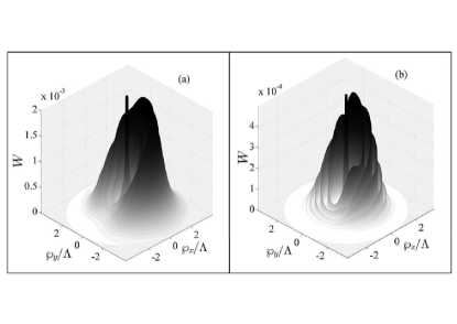
Figure 2: Atomic momentum distribution against $\wp_{x}/\Lambda\times$ $\wp_{y}/\Lambda$ for (a) $\Lambda=5$ and (b) $\Lambda=20$. Simulations realized for $k\Delta r=2\pi/10$, with the atoms initially prepared in the superposition $\left(\left|g\right\rangle+\operatorname*{e}\nolimits^{i\pi/3}\left|e\right\rangle\right)/\sqrt{2}$, and the cavity modes $a$ and $b$ in the product of coherent states $\left|\psi_{field}\right\rangle=\left|\alpha\right\rangle\otimes\left|\beta\right\rangle$, with $\alpha=\beta\operatorname*{e}\nolimits^{i\pi/2}=1.5\operatorname*{e}\nolimits^{i\pi/2}$.

To illustrate the role of the interaction parameter in the momentum distribution function, in Fig. 2 we display the 2D momentum distribution in the dimensionless space $\wp_{x}/\Lambda\times$ $\wp_{y}/\Lambda$, computed for the interaction parameters (a) $\Lambda=5$ and (b) $\Lambda=20$. As expected, the resolution of the distribution function becomes better as the interaction parameter $\Lambda$ is increased HAS ; FH ; BB . Moreover, the components of transverse momentum acquired by the atoms are given by a summation over the Fourier transforms $F_{m,n}(\wp,\phi)$, which, because of their dependence on the $\operatorname*{e}\nolimits^{-i\rho\left[\wp\cos(\theta-\phi)-\sqrt{n}\Lambda\right]}$ term (see Eq. (6)), each yield a radial transverse momentum of the atoms $\wp=\sqrt{n}\Lambda$, with $n\leq N$.

Another important feature visible in Fig. 2 is that the phase factor in the prepared atomic state is responsible for the asymmetry of the distributions, here favoring the probabilities on the first and second quadrant of $\wp_{x}/\Lambda\times$ $\wp_{y}/\Lambda$. As shown below, this asymmetry of the distribution is an important ingredient to achieve atomic lithography. Here we stress that the necessary presence of the ground state in the atomic superposition produces a great number of atoms with no significant deflection (see detailed discussion in Ref. Outro-Paper ), causing the distribution around the origin ($n=0$) to reach values considerably larger than those for $n>0$. Therefore, to highlight the discrete pattern of peaks for $n>0$, which corresponds to atoms that have indeed interacted with the cavities light, we have cut off in Fig. 2 the distributions around the origin, for $W>2\times 10^{-3}$ in Fig. 2(a) and $W>5\times 10^{-4}$ in Fig. 2(b). Based on the same reasoning, we have neglected the distribution around the origin for purposes of lithography.

We also observe in Fig. 2 that, by increasing the interaction parameter $\Lambda$ and consequently the transverse momentum $\wp$, the atoms are scattered to a larger region of the momentum space, at the expense of decreasing probabilities. For this reason, for the purpose of litography, i.e., to concentrate the probability distribution around a desired spot, it is better to use small values of $\Lambda$. Assuming that the atoms are measured on a screen located at a distance $L$ from the cavities, the transverse displacement associated with each radius is giving by $r_{n}=\sqrt{n}\Lambda\hbar kL/mv$, where $v$ is the longitudinal atomic velocity. With $L\sim 0.5$m and typical $v\sim 500$m/s, we obtain in the microwave regime: $r_{n}\sim\sqrt{n}\Lambda/10$, giving radii on the nanometer scale for an interaction parameter $\Lambda\sim 10$, that are separated by decreasing distances $r_{n+1}-$ $r_{n}\sim\left(\sqrt{n+1}-\sqrt{n}\right)\Lambda/10$ nm between concentric radii. This scheme provides subwavelength resolution in the nanometer scale using microwaves, for a wide range of photon number demanding the field to be treated in a quantum way.

While the cross-cavity OSG setup can be applied to two-mode tomography Outro-Paper , this device was designed from the start for the purpose of atomic lithography. After all, it seems quite reasonable to expect to be able to control the 2D deflection of the atomic beam by manipulating the cavity-mode states. Pursuing this initial goal, our protocol to achieve atomic lithography follows precisely from the manipulation of the amplitudes and phases of coherent $\left|\alpha\right\rangle$ or squeezed coherent $S_{\xi}\left|\alpha\right\rangle=\left|\alpha_{\xi}\right\rangle$ states ($\xi=r\operatorname*{e}\nolimits^{i\varphi}$ standing for the squeeze parameters, with $\xi=0$ for the coherent state) previously prepared in both cavity modes. As we shall now show, this manipulation enables us to modulate the atomic distribution by concentrating this function around a desired spot. To this end, we resort to a map that associates the (real) transverse momentum components $\wp_{x},\wp_{y}$ acquired by the atoms with the field states prepared in the two cavities, $a$ and $b$, which must be confined to their (abstract) momentum-quadrature components, i.e., $\alpha_{\xi}=\operatorname*{e}\nolimits^{i\varphi_{\alpha}}\left|\alpha_{\xi}\right|$ and $\beta_{\xi^{\prime}}=\operatorname*{e}\nolimits^{i\varphi_{\beta}}\left|\beta_{\xi^{\prime}}\right|$, with $\varphi_{\alpha},\varphi_{\beta}=\pm\pi/2$, respectively. While the choice of phases defines the quadrant in which the maximum of the atomic distribution is located: $\alpha_{\xi}=i\left|\alpha_{\xi}\right|$ and $\beta_{\xi^{\prime}}=i\left|\beta_{\xi^{\prime}}\right|$ defining the first quadrant of the space $\wp_{x}\times$ $\wp_{y}$, $\alpha_{\xi}=-i\left|\alpha_{\xi}\right|$ and $\beta_{\xi^{\prime}}=i\left|\beta_{\xi^{\prime}}\right|$ defining the second quadrant and so on, the amplitudes $\left|\alpha_{\xi}\right|$ and $\left|\beta_{\xi^{\prime}}\right|$, and consequently the mean values $\bar{\alpha}_{\xi}=\left\langle\alpha_{\xi}\right|a^{\dagger}a\left|\alpha_{\xi}\right\rangle$ and $\bar{\beta}_{\xi^{\prime}}=\left\langle\beta_{\xi^{\prime}}\right|b^{\dagger}b\left|\beta_{\xi^{\prime}}\right\rangle$, define the average radius and angle of the maximum of the atomic distribution. More specifically, we obtain the relations

$$\bar{\wp} =\left(\bar{\wp}_{x}+\bar{\wp}_{y}\right)^{1/2}\approx\Lambda\left(\bar{\alpha}_{\xi}+\bar{\beta}_{\xi^{\prime}}\right)^{1/2}\text{,}$$ (9a)

$$\bar{\phi} \approx\operatorname*{sign}(\varphi_{\alpha})\operatorname*{sign}(\varphi_{\beta})\tan^{-1}\sqrt{\bar{\beta}_{\xi^{\prime}}/\bar{\alpha}_{\xi}}+\pi\delta_{\varphi_{\alpha},-\left|\varphi_{\beta}\right|}\text{.}$$ (9b)

The quantum nature of the fields reveals itself in the discrete peaks with mean momentum $$\sqrt{n}\Lambda n \left\langle n\right\rangle\approx\bar{\alpha}_{\xi}+\bar{\beta}_{\xi^{\prime}} \bar{\wp}_{x}\approx\Lambda\bar{\alpha}_{\xi} \bar{\wp}_{y}\approx\Lambda\bar{\beta}_{\xi^{\prime}}$$. Since the expectation value of is approximately the average total number of photons in the cavities , we infer that and , and consequently Eqs. (9a) and (9b).

Apart from the manipulation of the cavity mode states, we must stress that the phase factor appearing in the prepared atomic superposition $\left(\left|g\right\rangle+\operatorname*{e}\nolimits^{i\varkappa}\left|e\right\rangle\right)/\sqrt{2}$ is another important ingredient for the achievement of atomic litography. We have found that the choice $\varkappa=\pi/2$ maximizes the distribution around the desired $\bar{\wp}$ and $\bar{\phi}$, so it will be adopted in our illustration of the lithography process.

We begin by showing the effectiveness of the map in Eq. (9) and by discussing the resolution of the atomic beam deflection —its sharpness around the desired spot— achieved when coherent or squeezed coherent states are prepared in both cavity modes. We demonstrate that the more a coherent state is squeezed in the momentum quadrature, the better the resolution becomes. Furthermore, besides the need to confine the fields to their momentum-quadrature components, their squeezing must also be done in the same field quadrature, i.e., $\varphi=\pi$.

In Fig. 3(a) we present the momentum distribution following from the coherent states $\alpha_{0}=\beta_{0}=3.54i$, with $\Lambda=4$. We clearly observe a peak located around the desired values $\bar{\wp}=20$ and $\bar{\phi}=\pi/4$, in excellent agreement with the values derived from Eq. (9). A view from above of this momentum distribution is also presented (again disregardeding the corresponding probabilities around the center), which seems to be more convenient for tomographic purposes.

In Fig. 3(b), the atomic momentum distribution resulting from a squeezed state generated from $\alpha$ $=$ $\beta=5.77i$ and with squeezing factors $r=r^{\prime}=0.5$ (other parameters being the same as in Fig. 3(a)), is presented, exhibiting a higher resolution achieved around the same target $\bar{\wp}=20$ and $\bar{\phi}=\pi/4$. Indeed a sharper peak of the momentum distribution is located around the desired spot. The region of the distribution function concentrating substantial probabilities around the desired spot has decreased significantly. By increasing further the squeezing factors to $r=r^{\prime}=1$, and using $\alpha$ $=$ $\beta=9.06i$ to keep $\bar{\wp}=20$ and $\bar{\phi}=\pi/4$, we observe in Fig. 3(c) that the resolution of the distribution is further enhanced.

Next, we demonstrate how to manipulate the radial and angular degrees of freedom of the atomic deflection. Once more assuming $\Lambda=4$ and squeezed states generated from $\alpha$ $=$ $5.7i$ and $\beta$ $=$ $7.1i$, with $r=r^{\prime}=1$, in Fig. 4(a) we present the distribution associated with the target $\bar{\wp}=15$ and $\bar{\phi}=5\pi/18$, showing that smaller values of the radii $\bar{\wp}$ may be achieved. Although values of $\bar{\wp}$ larger than $20$ may also be accessed, we limited ourselves to $\bar{\wp}\leq$ $20$ because of the large computational demand to compute Eq. (2). Finally, in Fig. 4(b), we take the same parameters as in Fig. 4(a), but squeezed states generated from $\alpha$ $=$ $-5.7i$ and $\beta$ $=$ $7.1i$, associated with the rotated target $\bar{\wp}=15$ and $\bar{\phi}=13\pi/18$.

In conclusion, we have thus presented a full quantum mechanical scheme for atomic lithography and demonstrated its effectiveness and tunability. We stress that, differently from previous set-ups, the cavity set-up provides a tunable lithographic scheme, in the sense that it is sufficient to tune the intracavity field to monitor the deflection angle of the atomic beam. Then, the cross-cavity allows to reach full two-dimensional control of the beam deviation since each cavity offers control over one spatial degree of freedom. In particular, mask-based techniques require designing a specific mask for each atomic pattern — the light-based scheme requires only to tune the fields to create a new pattern. Practically, it may be used to design two-dimensional microstructures. It is worth stressing that our aim is not to compare the performance of our quantum scheme with semiclassical atomic lithography, but to demonstrate the possibility of building effective potentials from the radiation-matter interaction alone. The methods developed above also enable the simultaneous tomography of two-mode states, by measuring the 2D atomic momentum distribution Outro-Paper . We finally observe that the 2D cross-cavity OSG can also be used to generate Schrödinger-cat atomic states and entangled atomic states in positional space, a goal that we will pursue at the next step.

Acknowledgements

The authors thanks V. S. Bagnato and B. Baseia for suggesting the theme, and C. J. Villas-Bôas and S. S. Mizrahi for enlightening discussions. We also acknowledge the support from PRP/USP within the Research Support Center Initiative (NAP Q-NANO) and FAPESP, CNPQ and CAPES, Brazilian agencies.

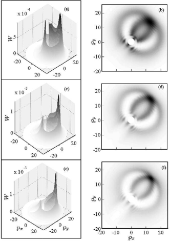
Figure 3: Atomic momentum distribution for $\Lambda=4$, $k\Delta r=2\pi/10$, the atoms prepared in the superposition state $\left(\left|g\right\rangle+\operatorname*{e}\nolimits^{i\pi/2}\left|e\right\rangle\right)$, and the cavity modes in the (a) coherent states $\alpha_{0}=\beta_{0}=3.54i$, (b) squeezed coherent states with $\alpha$ $=$ $\beta=5.77i$ and squeezing factors $r=r^{\prime}=0.5$, and (c) squeezed coherent states with $\alpha$ $=$ $\beta=9.06i$ and squeezing factors $r=r^{\prime}=1$. In all three cases we aim at the target $\bar{\wp}=20$ and $\bar{\phi}=\pi/4$.

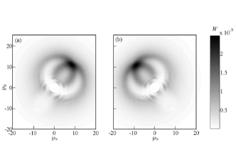
Figure 4: Atomic momentum distribution for $\Lambda=4$, $k\Delta r=2\pi/10$, the atoms prepared in the superposition state $\left(\left|g\right\rangle+\operatorname*{e}\nolimits^{i\pi/2}\left|e\right\rangle\right)$, and the cavity modes in the squeezed states generated from the squeezing factors $r=r^{\prime}=1$, with (a) $\alpha$ $=$ $5.7i$ and $\beta$ $=$ $7.1i$ and (b) $\alpha$ $=$ $-5.7i$ and $\beta$ $=$ $7.1i$.

References

- (1) Experimental demonstration of the optical Stern-Gerlach effect, T. Sleator, T. Pfau, V. Balykin, O. Carnal, and J. Mlynek, Phys. Rev. Lett. 68, 1996 (1992).
- (2) Quantum demolition measurement of photon statistics by atomic beam deflection, A. M. Herkommer, V. M. Akulin, and W. P. Schleich, Phys. Rev. Lett. 69, 3298 (1992).
- (3) Probing a Quantum State via Atomic Deflection, M. Freyberger and A. M. Herkommer, Phys. Rev. Lett. 72, 1952 (1994).
- (4) Scattering of atoms by light - Probing a quantum state and the variance of the phse operator, B. Baseia, R. Vyas, C. M. A. Dantas, V.S. Bagnato, Phys. Lett. A 194, 153 (1994).
- (5) Quantum features of the pondermotive meter of electromagnetic energy, V. B. Braginskyand F. Y. Khalili, Sov. Phys. JETP 46, 705 (1977).
- (6) Determination of quasiprobability distributions in terms of probability distributions for the rotated quadrature phase, K. Vogel and H. Risken, Phys. Rev. A 40, 2847 (1989).
- (7) Quantum non-demolition detection of single microwave photons in a circuit, B. R. Johnson, M. D. Reed, A. A. Houck, D. I. Schuster, Lev S. Bishop, E. Ginossar, J. M. Gambetta, L. DiCarlo, L. Frunzio, S. M. Girvin & R. J. Schoelkopf, Nature Phys. 6, 663 (2010).
- (8) Atom localization and center-of-mass wave-function determination via multiple simultaneous quadrature measurements, J. Evers, S. Qamar, and M. S. Zubairy, Phys. Rev. A 75, 053809 (2007).
- (9) Visualization of superposition states and Raman processes with two-dimensional atomic deflection, G. A. Abovyan , G. P. Djotyan, and G.Yu. Kryuchkyan, Phys. Rev. A 85, 013846 (2012).
- (10) Rotating optical cavity experiment testing Lorentz invariance at the 10-17 level, S. Herrmann, A. Senger, K. Möhle, M. Nagel, E. V. Kovalchuk, and A. Peters, Phys. Rev. D 80, 105011 (2009).
- (11) One-, two- and three-dimensional nanostructures with atom lithography, M. K. Oberthaler and T. Pfau, J. Phys. Condens. Matter 15, R233 (2003); Atomic nanofabrication: atomic deposition and lithography by laser and magnetic forces, D. Meschede and H. Metcalf, J. Phys. D 36, R17–R38 (2003); Nanotechnology with atom optics, J. J. McClelland, S. B. Hill, M. Pichler, R. J. Celotta, Sci. Technol. Adv. Mater. 5, 575 (2004).
- (12) Quasiperiodic structures via atom-optical nanofabrication, E. Jurdik, G. Myszkiewicz, J. Hohlfeld, A. Tsukamoto, A. J. Toonen, A. F. van Etteger, J. Gerritsen, J. Hermsen, S. Goldbach-Aschemann, W. L. Meerts, H. van Kempen, and Th. Rasing, Phys. Rev. B 69, 201102(R) (2004).
- (13) Atom Lithography with a Holographic Light Mask, M. Mützel, S. Tandler, D. Haubrich, D. Meschede, K. Peithmann, M. Flaspöhler, and K. Buse, Phys. Rev. Lett. 88, 083601 (2002); Atomic nanofabrication with complex light fields, M. Mützel, U. Rasbach, D. Meschede, C. Burstedde, J. Braun, A. Kunoth, K. Peithmann and K. Buse, Appl. Phys. B 77, 1 (2003).
- (14) Two-dimensional atomic lithography by submicrometer focusing of atomic beams, W. Williams and M. Saffman, J. Opt. Soc. Am. B 23, 1161 (2006).
- (15) Quantum lens for atomic waves, I. Sh. Averbukh, V. M. Akulin, and W. P. Schleich, Phys. Rev. Lett. 72, 437 (1994).
- (16) Quantized light lenses for atoms: The perfect thick lens, B. Rohwedder and M. Orszag, Phys. Rev. A 54, 5076 (1996).
- (17) W.P. Schleich, Quantum Optics in Phase Space (Wiley-VCH, New York, 2001).
- (18) Atom de Broglie Wave Deflection by a Single Cavity Mode in the Few-Photon Limit: Quantum Prism, P. Domokos, P. Adam, J. Janszky, and A. Zeilinger, Phys. Rev. Lett. 77, 1663 (1996).
- (19) Phys. Rev. A 79, 013421 (2009), O. Steuernagel, Phys. Rev. A 79, 013421 (2009) and refs. therein.
- (20) Simultaneous tomography of two-mode states via cross-cavity optical Stern-Gerlach Setup, C. E. Máximo, T. B. Batalhão, R. Bachelard, G. D. de Moraes Neto, M. A. de Ponte, and M. H. Y. Moussa, to be published elsewhere.