Composition analysis based on Bayesian methods

Abstract

In this work we test the most widely used methods for fitting the composition fraction in data, namely maximum likelihood, $\chi^{2}$, mean value of the distributions and mean value of the posterior probability function. We discuss the discrimination power of the four methods in different scenarios: signal to noise discrimination; two signals; and distributions of Xmax for mixed primary mass composition. We introduce a "distance" parameter, which can be used to estimate, as a rule of thumb, the precision of the discrimination. Finally, we conclude that the most reliable methods in all the studied scenarios are the maximum likelihood and the mean value of the posterior probability function.

I Introduction

One of the main challenges of the astroparticle physics reasearch is to determine the chemical composition of the cosmic rays that reach the earth. At the highest cosmic ray energies, analysis of composition must be made with indirect methods by using the evolution of cosmic ray showers in the atmosphere. In this note, we use four different methods to estimate the composition given a single variable (e.g. the $X_{\rm max}$ distribution) by using Bayesian methods. A similar work, using Monte Carlo techniques, to study the efficiency of different discriminators can be found in Durso .

The note is as follows: in section II we discuss the four different methods and we apply them in simple analytical cases in section II.1. In section III, we apply the different methods to two physical cases Signal to Noise discrimination and two overlapped signals. Finally, we evaluate the methods for the specific example of $X_{\rm max}$ distributions with realistic probability densities and we get a possible composition of the cosmic rays in section IV.

To be concrete, we will consider a two composition scenario. Although the methods discussed can be easily generalized to include more than two distributions.

II Methods

Consider the following problem. A given data variable is extracted from two different probability distributions with a “composition” fraction $\alpha$, ($0\leq\alpha\leq 1$) so that the joint probability distribution is given by

$$f(x;\alpha)=\alpha g_{1}(x)+(1-\alpha)g_{2}(x).$$ (1)

The probability distributions $g_{1,2}(x)$ are known and the problem consists in determining the composition fraction $\alpha$ from the measurement of $n$ data points $x_{i}$, $i=1,\cdots,n$. If $\alpha$ was known, the probability of getting the data $D=\{x_{i}\}$ is given by

$$P(D|\alpha I)=\prod_{i=1}^{n}f(x_{i};\alpha),$$ (2)

where $I$ is any prior information we have about the problem, including the prescription of the probabilities $g_{i}$. Here we are implicitly assuming that the different data points are independent. Using Bayes’s theorem Evans , we can obtain the posterior probability for $\alpha$ given the data

$$P(\alpha|DI)=\frac{P(D|\alpha I)P(\alpha|I)}{P(D|I)}.$$ (3)

$P(D|I)$ is the probability of obtaining the given data independently of any value of $\alpha$ and here acts as a normalization constant. $P(\alpha|I)$ is the prior probability for $\alpha$. In our problem, astrophysical input may give information on the cosmic ray composition and give preference for, say, proton domination. In the absence of any information a flat distribution gives good results. In the following we will use $P(\alpha|I)=1$ but all our results will be valid for other choices of prior probabilities. Therefore, we can write Eq.(3) as

$$P(\alpha|DI)=\frac{1}{\mathcal{N}}\prod_{i=1}^{N}\left\{\alpha g_{1}(x_{i})+(1-\alpha)g_{2}(x_{i})\right\},$$ (4)

where $\mathcal{N}$ is a normalization constant. In some problems instead of Eq. (4), where all the data points are given, one has data binned in the variable $x$. In that case the equation reads

$$P(\alpha|D_{k}I)=\frac{1}{\mathcal{N}}\prod_{j=1}^{k}\left\{\alpha G_{1}(x_{j})+(1-\alpha)G_{2}(x_{j})\right\}^{n_{k}},$$ (5)

where the data now is $D_{k}=\{n_{1},\cdots,n_{k}\}$, the number of events in the bins $1,\cdots,k$ with center values $x_{1},\cdots,x_{k}$, and $G_{i}(x_{j})=\int_{x_{j}}g_{i}(x)dx$ is the integral on the bin of the probability density. Although binning the data makes the problem somehow easier, it wastes information.

Eq. (4) (or alternatively Eq. (5)) contains all the information we have about our problem. Estimation of the composition fraction reduces to the choice of a “best estimator”. Now we examine the different choices which are currently used in the literature.

• $\alpha_{<>}$

  We can calculate the mean of the data points and choose $\alpha$ such that it coincides with the mean value of the distributions, i.e. if $\bar{x}=\frac{1}{n}\sum_{i=1}^{n}x_{i}$, then

  $$\bar{x}=\alpha\left\langle g_{1}(x)\right\rangle+(1-\alpha)\left\langle g_{2}(x)\right\rangle$$ (6)

  if we define $\bar{x}_{i}=\int xg_{i}(x)dx$, then we get

  $$\alpha_{<>}=\frac{\bar{x}-\bar{x}_{2}}{\bar{x}_{1}-\bar{x}_{2}}.$$ (7)

  Eq. (7) has a simple analytical form and is easy to evaluate for any distribution (provided it has first moments). This is a useful advantage when working with the first few moments (see e.g. Abreu ). However, it can give unphysical results (($\alpha>1$, $\alpha<0$) and gives the largest deviation with respect to the true value for all studied estimators.

• $\alpha_{\rm max}$

  Alternatively, one can choose as the best estimator, the value that maximizes the posterior probability.

  $$\frac{\partial P(\alpha|DI)}{\partial\alpha}=0.$$ (8)

  Since $P(\alpha)$ is positive an equivalent alternative is to maximize the logarithm of $P$. Then

  $$\frac{\partial\log P(\alpha|DI)}{\partial\alpha}=\sum_{i=1}^{n}\frac{g_{1}(x_{i})-g_{2}(x_{i})}{\alpha g_{1}(x_{i})+(1-\alpha)g_{2}(x_{i})}=0.$$ (9)

  This is the maximum likelihood estimation. It is known to give very good estimation of $\alpha$ in almost all cases, even for small number of events. It has the disadvantage that an analytical solution is possible only for very small number of events or bins. This method is used, for instance, in the standard package TFractionFitter of ROOT TFitter . Usually, the solution is found by numerically searching for the maximum of Eqs. (8,9).

• $\alpha_{\chi}$

  If the number of events is large, one expects a well defined peak distribution in $\alpha$. Near the maximum of the distribution one can approximate this distribution by a gaussian. Binning the data we can construct a $\chi^{2}$ variable for the problem

  $$\chi^{2}(\alpha)=\sum_{j=1}^{k}\frac{(n_{j}/n-F(x_{j},\alpha))^{2}}{n_{j}},$$ (10)

  where $n_{j}$ is the number of data events in bin $j$ and $F(x_{j},\alpha)=\alpha G_{1}(x_{j})+(1-\alpha)G_{2}(x_{j})$ is the probability of having an event in bin $j$ for a given $\alpha$. The optimal value of $\alpha$ can be found minimizing the $\chi^{2}$

  $$\frac{\partial\chi^{2}(\alpha)}{\partial\alpha}=0.$$ (11)

  The solution of Eq. ((11)) has the advantage of being an analytical and relatively simple expression

  $$\alpha_{\chi}=\frac{\sum_{j=1}^{k}(n_{j}/n-G_{2}(x_{j}))(G_{1}(x_{j})-G_{2}(x_{j}))}{\sum_{j=1}^{k}(G_{1}(x_{j})-G_{2}(x_{j}))^{2}}.$$ (12)

  It is an asymptotic limit (for $n$ and $n_{j}$ large) of the maximum likelihood method and, as such, gives very good results in this limit.

• $\left\langle\alpha\right\rangle$

  Once we know the probability density function for $\alpha$, we can obtain the mean value of the distribution

  $$\left\langle\alpha\right\rangle=\int_{0}^{1}d\alpha\;\alpha\;P(\alpha|DI).$$ (13)

  Although this estimator is not much used, we will shown below that it gives the best performance in most cases. It has the disadvantage of being difficult to evaluate analytically but for the simplest cases.

• $\alpha_{M}$

  Any other estimator could provide sensible results. As an example, the median of the posterior probability, defined by

  $$\int_{0}^{\alpha_{M}}d\alpha P(\alpha|DI)=\int_{\alpha_{M}}^{1}d\alpha P(\alpha|DI)=1/2.$$ (14)

  It is well known that the median is a robust estimator, being invariant against a large set of transformations of the probability distributions. However, it is difficult to evaluate both analytically and numerically. Therefore we do not consider it any further.

II.1 A toy analytical case: heads or tails

The simplest problem of discrimination is the following: Assume that the two distributions $g_{1}(x)$ and $g_{2}(x)$ are totally separated (i.e. they do not overlap). In that case, the actual shape of $g_{1}$ and $g_{2}$ is irrelevant and one can bin the data in just two bins $x=a,b$ such that all the probability is concentrated in either bin $a$ or $b$. So, let the two probability functions be

$$G_{1}(x)=\left\{\begin{matrix}1&\mbox{if }x=a\\ 0&\mbox{if }x=b\end{matrix}\right.$$ (15)

$$G_{2}(x)=\left\{\begin{matrix}0&\mbox{if }x=a\\ 1&\mbox{if }x=b\end{matrix}\right.$$ (16)

Denoting $\phi(\alpha)=P(\alpha|DI)$ and applying Eq. (4), then

$$\phi(\alpha)=\frac{1}{\mathcal{N}}\left[\alpha^{n}(1-\alpha)^{N-n}\right]$$ (17)

where $n$ is the number of events with $x=a$ and $N-n$ is the number of events with $x=b$, and $N$ the total number of events. This is just a problem of determining the probability of having heads or tails in a (possibly) loaded coin given the number of heads and tails in an experiment. As could be expected, it is just a binomial distribution.

By direct calculation, one obtains

$$\alpha_{\chi}=\alpha_{\rm max}=\alpha_{<>}=\frac{n}{N}.$$ (18)

We obtain as the estimation of the probability of “head” events, the fraction of head events observed. On the other hand the mean $\alpha$ gives

$$\left\langle\alpha\right\rangle=\frac{n+1}{N+2}.$$ (19)

Although this result may be surprising at first sight it is a well known result in the literature. It is known as Laplace’s succession rule. One may notice that in the limit $N,n\rightarrow\infty$ with $n/N$ fixed one recovers Eq. (18). Note that if $N=0$, then $n=0$ and all the methods are indefinite except the mean value which gives $\frac{1}{2}$. This is just the mean value of the prior probability. If $N=1$, then either $n=0$ or $n=1$, which would give either $\alpha_{\rm max}=0$ or $1$. Eq. (19) gives $\left\langle\alpha\right\rangle=1/3$ or $2/3$. In section III we show numerically this phenomenon for a more realistic model.

II.2 Heads or tails with contamination

For a more interesting case, consider now the previous example but with a (possibly small) contamination between both distributions

$$G_{1}(x)=\left\{\begin{matrix}1-\epsilon&\mbox{if }x=a\\ \epsilon&\mbox{if }x=b\end{matrix}\right.$$ (20)

$$G_{2}(x)=\left\{\begin{matrix}\delta&\mbox{if }x=a\\ 1-\delta&\mbox{if }x=b\end{matrix}\right.$$ (21)

So that there is a (small) probability of a event of type 1 (“heads”) to be identified in the bin 2 (“tails”) and vice-versa. The posterior probability, after measuring $N=n_{1}+n_{2}$ total events with $n_{1}$ of type 1 and $n_{2}$ of type 2 is

$$\phi(\alpha)=\frac{1}{\mathcal{N}}\left[\alpha(1-\epsilon)+(1-\alpha)\delta\right]^{n_{1}}\left[\alpha\epsilon+(1-\alpha)(1-\delta)\right]^{n_{2}}.$$ (22)

After some algebra one obtains again

$$\alpha_{\chi}=\alpha_{\rm max}=\alpha_{<>}=\frac{1}{1-\delta-\epsilon}\left[\frac{n_{1}}{N}-\delta\right].$$ (23)

The mean value of $\alpha$ has not a simple analytical expression. It is given by

$$\left\langle\alpha\right\rangle=\frac{1}{1-\delta-\epsilon}\left(\frac{B(1-\epsilon,n_{1}+2,n_{2}+1)-B(\delta,n_{1}+2,n_{2}+1)}{B(1-\epsilon,n_{1}+1,n_{2}+1)-B(\delta,n_{1}+1,n_{2}+1)}\right)-\frac{\delta}{1-\delta-\epsilon},$$ (24)

where $B(x,n_{1},n_{2})$ is the incomplete Beta function Abramowitz

$$B(x,n_{1},n_{2})=\int_{0}^{x}dyy^{n_{1}-1}(1-y)^{n_{2}-1}.$$ (25)

For $n_{1}$ and $n_{2}$ integers $B$ is a polynomial in $x$. One can show that the above equation gives always physical values $0\leq\alpha\leq 1$, even for degenerate cases.

Although this model is rather simplistic, it has all the ingredients found in actual cases. One can interpret Eq. (23) rather easily, the term $-\delta$ subtract the expected fraction of events of type 2 which fall into bin 1. On the other hand the factor $1-\delta-\epsilon$ is a measure of the fraction of well identified events. It is also a measure of the overlapping of the two distribution. As we will see below, this is a general characteristic of the problem. Another interesting point of Eq. (23) is the fact that it can produce unphysical results. If $n/N<\delta$, the expected fraction is negative. This is so because even for $\alpha=0$, we expect a number of events in the first bin of $\delta N$. Finally, one can see that the case $\epsilon+\delta=1$ is ill defined. But in this case both distributions are equal: no discrimination can be made between the two distributions.

The mean value determination $\left\langle\alpha\right\rangle$ does not suffer from this behavior, always giving physically admissible results. In the case of the two distributions being equal, we would obtain $\left\langle\alpha\right\rangle=1/2$, which is easily interpreted. If the data can not differentiate between the two cases we do not gain any information from the data and the estimation given by our prior is kept.

III Application of the methods

We now apply the methods discussed previously to several different scenarios. In section III.1, we study a typical problem of signal/noise identification. In section III.2, we concentrate on the separation of two signals and we study the dependence of the resolution with respect to the distance between the two signals.

A number of distance measures for probabilities has been proposed in the literature. In the appendix VII we discuss some possibilities and justify the choice of the overlapping area, as our distance. Given two distributions $g_{1}(x)$ and $g_{2}(x)$ we define the distance between the two distribution as

$$d_{1}(g_{1},g_{2})=\int dx|g_{1}(x)-g_{2}(x)|.$$ (26)

Which ranges between 0 and 2. For $d_{1}=2$ the distributions do not overlap; for $d_{1}=0$ the distributions are equal. For the previous example of heads and tails, the distance is given by $d_{1}=2(1-\delta-\epsilon)$, which is the pre-factor appearing in (23).

III.1 Signal/Noise discrimination

Consider the case of extracting a signal with a well defined peak from events coming from the signal plus a flat noise. To be concrete, we will choose the following probability density functions

$$g_{1}(x)=\frac{1}{\cal N}\exp{\left\{-\frac{(x-\mu)^{2}}{2\sigma^{2}}\right\}};x\in[a+\epsilon,b-\epsilon],$$ (27)

$$g_{2}(x)=\frac{1}{b-a};x\in[a,b].$$ (28)

Here $[a,b]$ is the range of the variable. We take the signal to be different from zero in a subrange of this interval, defined by $\epsilon>0$. $\cal N$ is a normalization constant and $\mu$ and $\sigma$ are the mean and RMS of the gaussian. In the numerical calculations we will choose $a=0$, $b=7$, $\epsilon=1$, $\mu=2$, and $\sigma=0.2$. The distance $d_{1}$ for this case is $1.694$.

In Fig. (1) we show both probability density functions.

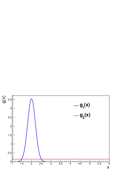
Figure 1: Probability density functions for signal and noise.

As a first numerical evaluation we calculate the estimated fraction for a true signal fraction of $\alpha=0.8$ with a fixed number of events of 30, 300 and 3000. In Fig. 2 we show the data in a typical run.

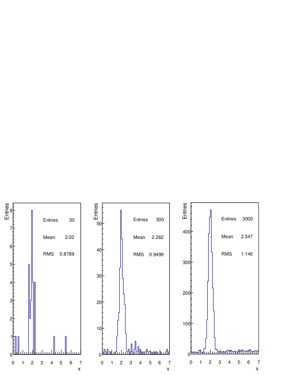
Figure 2: Data histograms for 30, 300 and 3000 events sampled from the distributions in Fig.1.

In table 1 we show the results for all estimators discussed and for the cases with different number of events. In Figures 3 and 4 we show the fraction probability and $\chi^{2}$ functions obtained.

# Events	$\left\langle\alpha\right\rangle$	$\alpha_{\rm max}$	$\alpha_{\chi^{2}}$	$\alpha_{<>}$
30	0.82	0.84	0.00	0.70
300	0.79	0.79	0.63	0.82
3000	0.80	0.80	0.81	0.78

Table 1: Results for the signal/noise discrimination.

Note that all of the methods give a reasonable fraction, but the mean value gives the estimated fraction closest to the true fraction. In this case, we can not choose a method or another, getting the same results except the $\chi^{2}$ method, which is the worst estimator for this example.

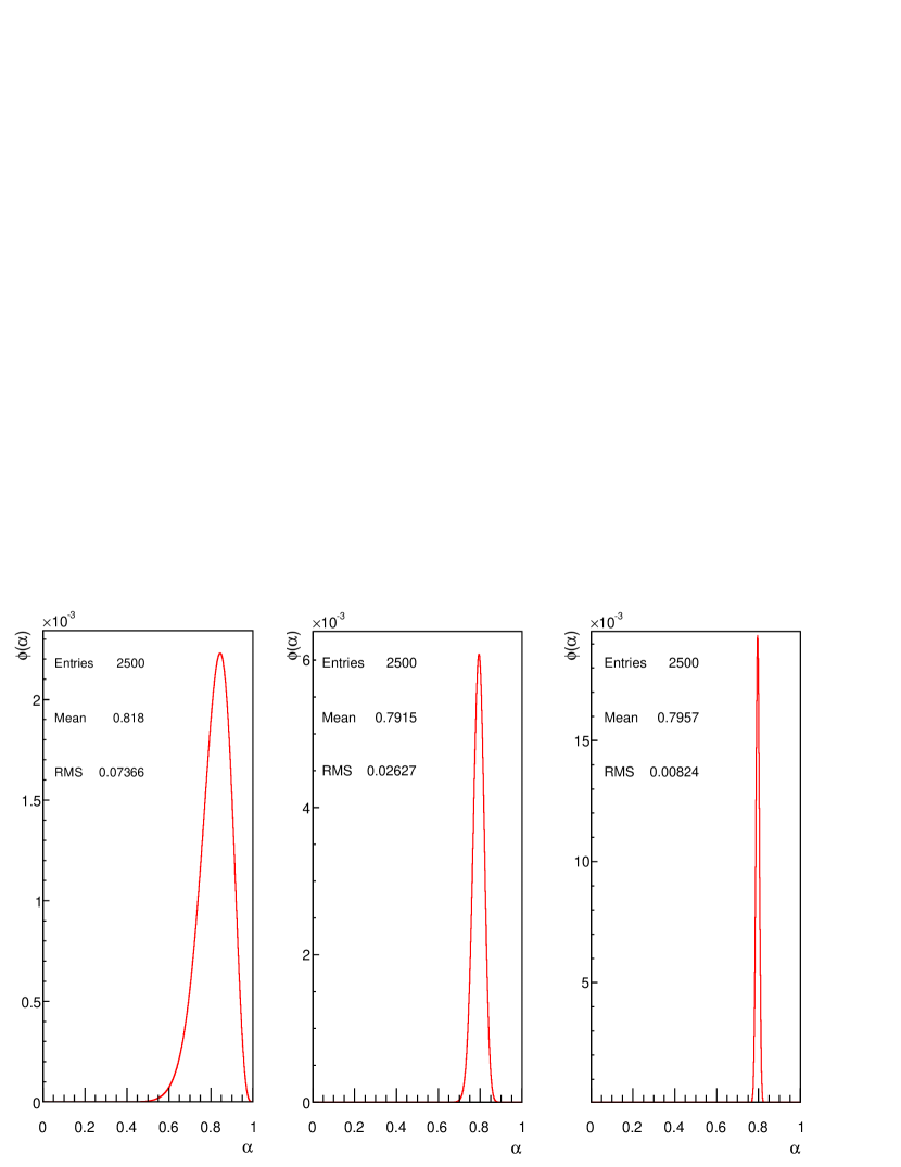
Figure 3: Probability functions of $\alpha$ for 30, 300 and 3000 events. The true fraction is 0.8

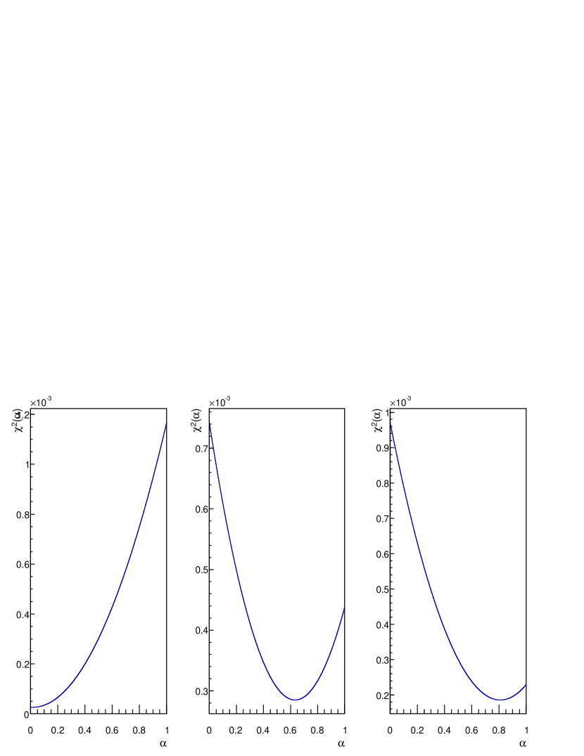
Figure 4: $\chi^{2}$ distributions for fixed number of events of 30, 300, and 3000. The true fraction is 0.8.

For the uncertainties we may take the RMS of the posterior probability functions. We obtain 0.07, 0.03 and 0.008 for 30, 300 and 3000 events. The $\chi^{2}$ estimator gives such a bad result due to the chosen binning. We have chosen a bin size of 0.002, which for small number of events is unreasonable. This was done on purpose to show that one does not need to bin the data and that binning can produce bad results, if poorly done.

III.2 Two signals

As a further example consider now the problem of discrimination of two signals which we will model as gaussians

$$g_{1}(x)=\frac{1}{\sigma_{1}\sqrt{2\pi}}\exp{\left\{-\frac{(x-\mu_{1})^{2}}{2\sigma_{1}^{2}}\right\}},$$ (29)

$$g_{2}(x)=\frac{1}{\sigma_{2}\sqrt{2\pi}}\exp{\left\{-\frac{(x-\mu_{2})^{2}}{2\sigma_{2}^{2}}\right\}}.$$ (30)

We will use $\mu_{1}=0$, $\sigma_{1}=1$, and $\sigma_{2}=0.5$. In our numerical examples, we vary $\mu_{2}$ from -1.5 to 1.5 to search for the efficiency of the methods for different distances between the probability distributions and we will also use different values of the composition fraction.

For gaussian distributions the distance between the two functions can be written as

$$d_{1}(g_{1},g_{2})=\int dx|g_{1}(x)-g_{2}(x)|=I_{1}+I_{2}+I_{3},$$ (31)

where the $I_{i}$ are combinations of error functions

$$I_{1}=\frac{1}{2}|{\rm Erf}(\frac{x_{c1}-\mu_{1}}{\sqrt{(}2)\sigma_{1}})-{\rm Erf}(\frac{x_{c1}-\mu_{2}}{\sqrt{(}2)\sigma_{2}})|,$$ (32)

$$I_{2}=\frac{1}{2}|{\rm Erf}(\frac{x_{c2}-\mu_{1}}{\sqrt{(}2)\sigma_{1}})-{\rm Erf}(\frac{x_{c1}-\mu_{1}}{\sqrt{(}2)\sigma_{1}})-{\rm Erf}(\frac{x_{c2}-\mu_{2}}{\sqrt{(}2)\sigma_{2}})+{\rm Erf}(\frac{x_{c1}-\mu_{2}}{\sqrt{(}2)\sigma_{2}})|,$$ (33)

$$I_{3}=\frac{1}{2}|{\rm Erf}(\frac{\mu_{1}-x_{c2}}{\sqrt{(}2)\sigma_{1}})-{\rm Erf}(\frac{\mu_{2}-x_{c2}}{\sqrt{(}2)\sigma_{2}})|,$$ (34)

and where $x_{c1,2}$ are the two solutions to the equation

$$g_{1}(x)=g_{2}(x).$$

We have run 10000 trials with 30, 300, and 3000 events for each value of the composition fraction, $\alpha_{true}$, varying from 0 to 1 in steps of 0.1. In figures 5-7 we show $|\alpha-\alpha_{true}|$ as a function of the distance for 30, 300, and 3000 events. Note that the best estimator is the mean value of the posterior probability. For a large number of events this estimator tends to the maximum likelihood, but for small number of events or small distances it performs slightly better.

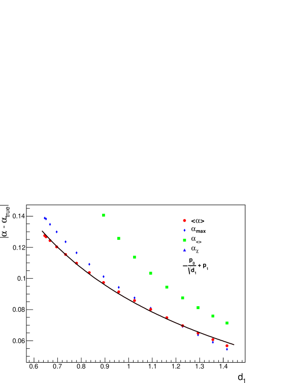
Figure 5: Absolute difference between the estimated fraction and true fraction for 30 data sample as a function of the distance. Note that $d_{1}=0$ means that the two distributions are equal while $d_{1}=2$ means that the distributions are completely separated.

Figure 6: Absolute difference between the calculated fraction and true fraction for 300 data sample as a function of the distance.

Figure 7: Absolute difference between the calculated fraction and true fraction for 3000 data sample as a function of the distance.

The $\chi^{2}$ method does not appear in figures 5 and 6, it is off scale due to the binning used in the estimation of the $\chi^{2}$. In figure 7 it is the worst method for the same reason. One can see in the same figures figures 5-7 that both $\left\langle\alpha\right\rangle$ and $\alpha_{max}$ scale as the squate root square of the distance. A fit to the function

$$|\alpha-\alpha_{true}|=\frac{p_{0}}{\sqrt{(}d_{1})}+p_{1},$$ (35)

is shown in the figures. This is in agreement with the results of section II.2 and confirms our choice for the distance. The uncertainty of $\alpha_{<>}$ more than double that of the maximum likelihood or the mean value for small distances. The corresponding RMS of the posterior probability distribution are shown in figure 8.

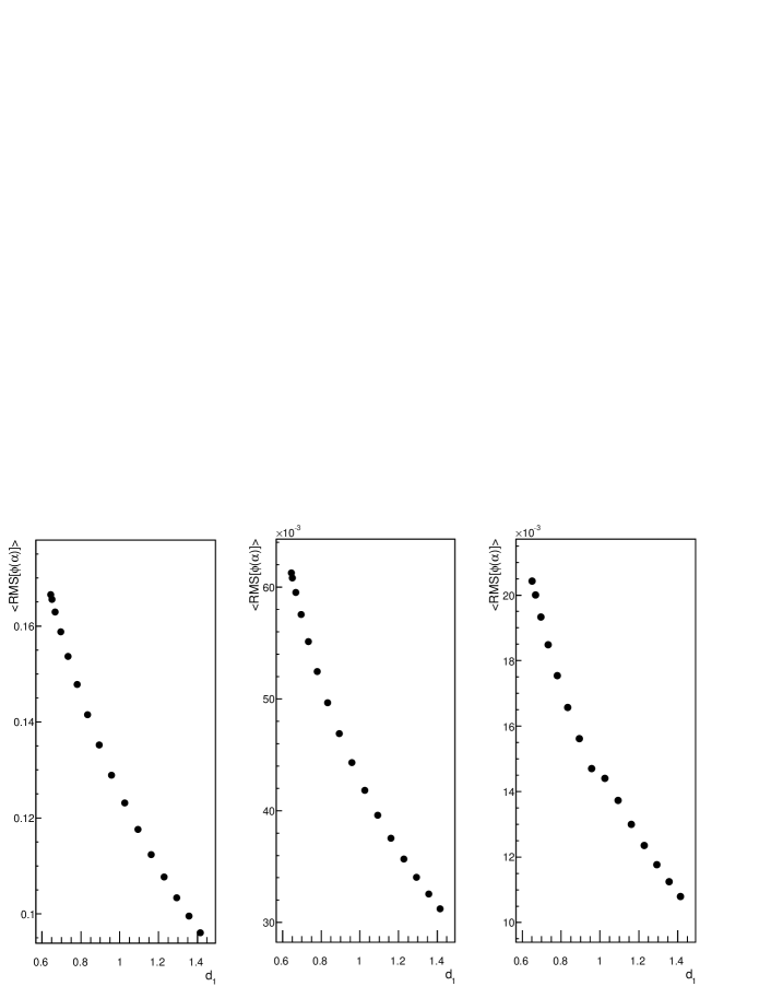
Figure 8: RMS of the posterior probability distribution for all trials as a function of the distance between the probability distributions. Left: analysis done with 30 events. Middle: 300 events. Right: 3000 events.

We now apply the methods for the gaussians with different mean and standard deviation for a single trial. In this case, we choose $\mu_{1}=2$, $\sigma_{1}=0.2$, $\mu_{2}=2.3$ and $\sigma_{2}=0.4$. The distance between the distributions is $d_{1}=0.926$. By looking at figures 5-7, we expect the fraction to be estimated with an uncertainty of $\sim 0.1$, $0.032$ and $0.001$ for 30, 300 and 3000 events respectively for the $\left\langle\alpha\right\rangle$ or $\alpha_{max}$ estimators. For the $\alpha_{<>}$ estimator we expect the uncertainty to be $<0.14$, $0.045$ and $0.014$.

In figure 9 we show the probability density functions for $g_{1}(x)$ and $g_{2}(x)$ considered here. Examples of data distributions are shown in figure 10.

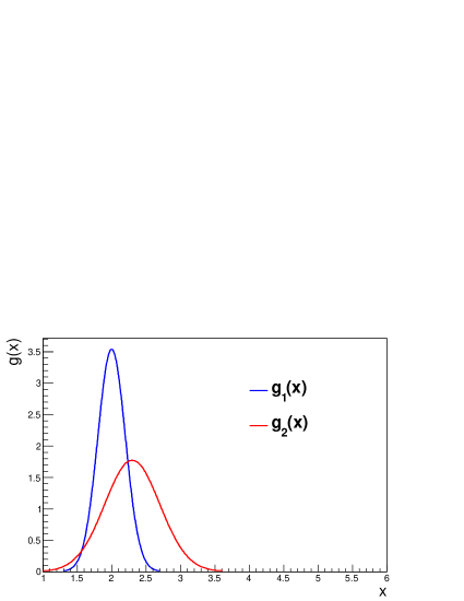
Figure 9: Probability density functions

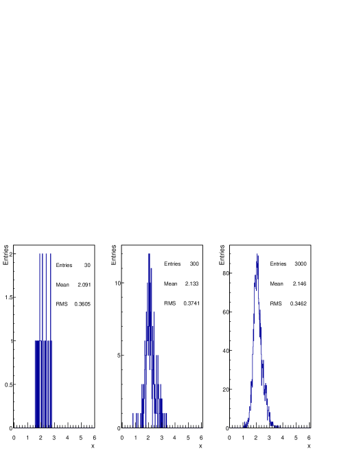
Figure 10: Data distributions analyzed for 30, 300 and 3000 events corresponding to the probability distributions in Fig. 9.

In table 2 we show the results for the four methods and figures 11 and 12 we show the probability distributions and the $\chi^{2}$ distributions.

# Events	$\left\langle\alpha\right\rangle$	$\alpha_{\rm max}$	$\alpha_{\chi^{2}}$	$\alpha_{<>}$
30	0.46	0.48	0.0	0.70
300	0.51	0.52	0.50	0.55
3000	0.51	0.51	0.54	0.51

Table 2: Results of the methods for the data samples. The true fraction is $\alpha_{true}=0.5$.

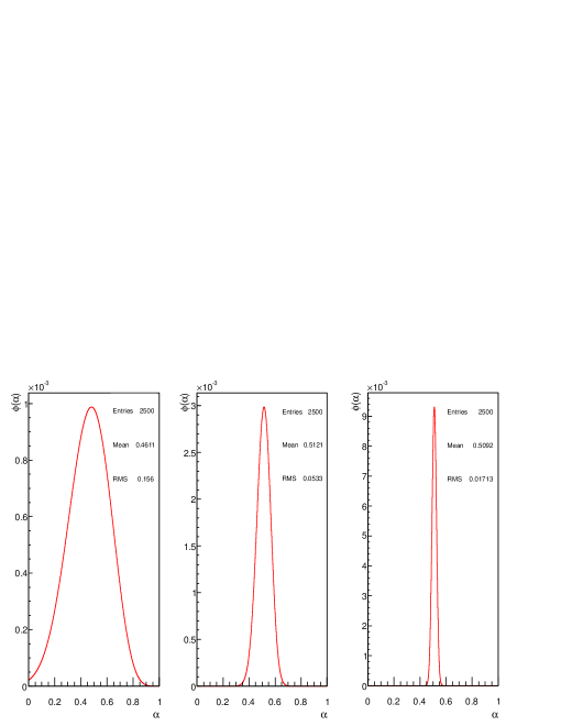
Figure 11: Posterior probability distributions of $\alpha$ for 30, 300, and 3000 events. The true fraction is $\alpha_{true}=0.5$.

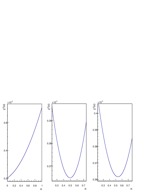
Figure 12: $\chi²$ functions for the same cases as figure 11.

IV Analysis of composition using $X_{\rm max}$ distributions

In the previous sections we have shown that the best estimators for the fraction are the mean value and maximum value of the probability distribution $P(\alpha|DI)$. We will now make an analysis of composition of the high energy cosmic rays using the maximum of the longitudinal profile, $X_{\rm max}$ as our discriminator Durso . We will use all the estimators discussed previously but concentrate on the results of the mean value and the maximum likelihood. The $X_{\rm max}$ distributions are generated with the CONEX generator using EPOS as the hadronic model.

Consider a typical example, where we want to find the proton and iron fraction in a data sample corresponding to energies between 1 EeV to 3.16 EeV. The distributions of $X_{\rm max}$ are shown in figure 13. The distance $d_{1}$ between the simulated distributions with the EPOS model in this energy bin is $1.55$, then, we can use, as a rule of thumb, our estimated resolution in the composition fraction to about $|\alpha-\alpha_{\rm true}|\sim 1/\sqrt{Nd_{1}}$ which amounts to 0.05, 0.012, or 0.006 for 30, 300, or 3000 events (see figures 5-7). The expected RMS of the distributions will be of order $\sigma\sim 0.1,0.03,0.01$ respectively.

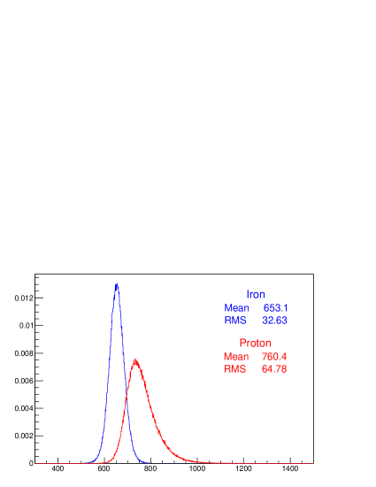
Figure 13: $X_{\rm max}$ distributions for Iron and Proton obtained from CONEX-EPOS with a primary energy from 1 EeV to 3.16 EeV.

In figure 14 we show the data distributions for three sample cases, with $\alpha=0.6$ and in figure 15 we show the corresponding posterior probability for these examples.

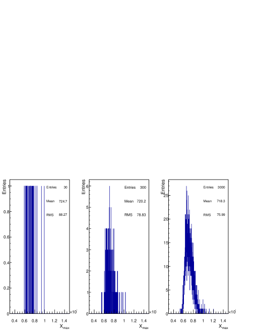
Figure 14: Sample data distributions analyzed for 30, 300, and 3000 events corresponding to the distributions in Fig.13.

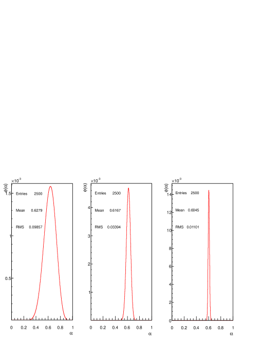
Figure 15: Posterior probability functions of $\alpha$ for 30, 300, and 3000 events.

In table 3, we show our results for these analysis, where the uncertainties are calculated in the following way: for the uncertainty in the mean value we take the RMS of the posterior distribution, for the uncertainty in the maximum likelihood value we take the width at $68\%$ confidence level.

# Events	$\left\langle\alpha\right\rangle$	$\alpha_{\rm max}$
30	$0.63\pm 0.10$	$0.64\pm 0.10$
300	$0.62\pm 0.03$	$0.62\pm\pm 0.03$
3000	$0.604\pm 0.010$	$0.604\pm 0.010$

Table 3: Composition fraction obtained with the mean and maximum values of the posterior probability function of $\alpha$. In this case $\alpha_{true}=0.6$.

In this example, both mean and maximum of the posterior probability give us the same results.

It has been suggested that one can eliminate partially the hadronic model dependence by shifting the mean values of the two distributions so that they coincide Facal ; Yushkov . However we expect that by centering the distributions one looses information to discriminate between the two compositions. The distance between the two distributions shown in fig. 13, if we center the two distributions is $d^{\prime}_{1}=0.62$ to be compared to the actual distance $d_{1}=1.55$. From our discussion, therefore, one expects a loss of resolution of the order $s=\sqrt{d^{\prime}_{1}/d_{1}}=0.63$, i.e. each event used in the discrimination with centering is worth a factor $s$ less than if used without centering. This has to be compared to the systematic uncertainty due to the hadronic model.

V Conclusions

We have studied different estimators for the evaluation of composition fraction between two distributions. We have shown that the best methods are the maximum and the mean of the probability distribution. The $\chi^{2}$ method gives results comparable to the maximum likelihood estimator, if the number of events is large, but by rebinning the results can be misleading. Also, we obtained the remarkable results that with few events, the mean value of the probability distribution is the best estimator.

We found a measure of distance between the two probabilities which gives us an estimation of the discrimination power for two distributions. If the distance $d_{1}$ is small, the discrimination between the two compositions will be poor. If the distance is large it will be optimal. We have shown that as a “rule of thumb” the discrimination power scales as $1/\sqrt{d_{1}N}$ with $N$ the number of events. Generalization of these methods to include an arbitrary number of components is straightforward and will be discussed separately.

VI Acknowledgments

We thank J. Alvarez-Muñiz, S. Riggi, I. Valiño, and E. Zas for discussions. We thank Alexey Yushkov for discussions and for pointing to us the relevance of centering the distributions. We thank Xunta de Galicia - Consellería de Educación (Grupos de Referencia Competitivos – Consolider Xunta de Galicia 2006/51); Ministerio de Educación, Cultura y Deporte (FPA 2010-18410 and Consolider CPAN - Ingenio 2010); Ministerio de Economía y Competitividad (FPA2012-39489), ASPERA - AugerNext (PRI-PIMASP-2011-1154) and Feder Funds, Spain. We thank CESGA (Centro de SuperComputación de Galicia) for computing resources.

VII Appendix A: Measures of distance

There are many measures of distance used in the literature. A much used measure of distance for probability distributions is the difference between the means

$$d_{\bar{x}}=\frac{\bar{x}_{1}-\bar{x}_{2}}{\sigma}.$$ (36)

where $\bar{x}_{i}$ is the mean value of $x$ for the two distributions and $\sigma$ is a measure of the width of the distributions (for instance, $\sigma^{2}=\sigma_{1}^{2}+\sigma_{2}^{2}$ has been used). It is however too restrictive. If $\bar{x}_{1}=\bar{x}_{2}$ then this distance is zero, suggesting that the two distributions can not be discriminated.

For two square integrable functions one can define the distance

$$d_{2}=\int dx(g_{1}(x)-g_{2}(x))^{2}.$$ (37)

This is much used in Physics, but for probability distributions is not useful, since it is not invariant against changes of variables.

A much used distance for probability distributions is the relative entropy distance, also known as the Kullback-Leibler Kullback-Leibler metric

$$d_{KL}=\int dxg_{1}(x)\log(g_{2}(x))-g_{2}(x)\log(g_{1}(x)).$$ (38)

For us, however, is not the relevant measure to use. It gives a distance of $\infty$ if there is a no-overlapping region ( $g_{2}(x)=0$ and $g_{1}(x)\neq 0$, for instance), which is the most relevant case in our problem.

We have found that the best choice of distance is that given by the overlapping area

$$d_{1}=\int dx|g_{1}(x)-g_{2}(x)|.$$ (39)

It measures somehow the amount of probability which is not “separable” between the two distributions. It is bounded between 0 and 2. $d_{1}=2$ implies that the two distributions do not overlap. $d_{1}=0$ means that the two distributions are equal.

References

- (1) D. D’Urso for the Pierre Auger Collaboration, “A Monte Carlo exploration of methods to determine the UHECR composition with the Pierre Auger Observatory”, arXiv:0906.2319 [astro-ph.CO]
- (2) M.J. Evans and J.S. Rosenthal, “Probability and Statistics: The Science of Uncertainty”, W.H. Freeman 2009.
- (3) R.J. Barlow and C. Beeston, “Fitting using finite Monte Carlo samples”, Compu. Phys. Commun. 77 (1993) 219.
- (4) M. Abramowitz and I.A. Stegun, “Handbook of mathematical functions”, Dover 1972.
- (5) P.Abreu et al. [Pierre Auger Collaboration], “Interpretation of the Depths of Maximum of Extensive Air Showers Measured by the Pierre Auger Observatory,” JCAP 1302 (2013) 026
- (6) P. Facal for the Pierre Auger Collaboration, “The distributions of shower maxima of UHECR air showers”, arXiv:1107.4804 [astro-ph.HE].
- (7) A. Yushkov, private communication.
- (8) S. Kullback and R.A. Leibler, “On information and sufficiency”, Ann. Math. Stat. 22 (1951) 79.