ABOUT HIERARCHY OF MULTIFREQUENCY QUASIPERIODICITY REGIMES IN DISCRETE LOW-DIMENSIONAL KURAMOTO MODEL

A dynamics of a low-dimensional ensemble consisting of connected in a network five discrete phase oscillators is considered. A two-parameter synchronization picture which appears instead of the Arnold tongues with an increase of the system dimension is discussed. An appearance of the Arnol’d resonance web is detected on the “frequency – coupling” parameter plane. The cases of attractive and repulsive interactions are discussed.

Keywords: quasiperiodicity; network of oscillators; Kuramoto transition; chart of Lyapunov exponents.

1 Introduction

Investigation of ensembles of interacting oscillators is an important problem with applications in various fields such as radiophysics, laser physics, biophysics, dynamics of gene networks, etc. [1, 2, 3, 4, 5]. Traditionally, the Kuramoto model which is used for this purposes represents a set of globally coupled phase oscillators [1, 2, 5, 6, 7, 8]. The main effect observed in this system is an appearance of a coherent state in the medium field generated by the ensemble (Kuramoto transition). However, the medium field model is efficient in case when the network contains a very large number of oscillators. At the same time, it is interesting to study a behavior of low-dimensional ensembles containing a relatively small number of oscillators. It is important for various applications, for example in biophysics when several subsystems with different natural rhythms interact with each other. This problem is also fundamental in the following context. Each new element addition into the system adds a new frequency. As a result, an emergence of high-dimensional quasiperiodic oscillations associated with the multi-dimensional invariant tori becomes possible. Variation of at least one fundamental frequency may initiate various resonant conditions. Due to the coupling of type “each-to-each”, the number of such resonances is maximal in the network of oscillators. With an increase in the coupling, hierarchy of resonances is observed. This is a situation when low-dimensional tori arise on the surfaces of high-dimensional tori. One can expect a complicated structure of such resonances. Thus, this problem may be interpreted as a generalization of the Arnol’d tongues to the multi-frequency systems.

At transition to systems with multi-frequency quasiperiodicity, however, we have to apply new methods of analysis. Indeed, it is necessary to identify quasiperiodic regimes of different dimensions and details of the internal organization of the domains of their existence. This problem can be solved by using a Lyapunov analysis, which should be performed at each point of the parameter plane. Then the analysis of the spectrum of Lyapunov exponents enables us to determine the type of regime. However, a solution of such a problem leads to the following difficulty. With an increase in number of oscillators a computation time required for the regime definition at each point in the parameter space becomes very large. This can be partially overcome by using a simple model and transition from the flow systems to the maps. The simplest method of map constructing is to replace time derivatives by finite differences in the dynamic equations. This approach is used, for example, in the conservative chaos theory (Chirikov–Taylor map) [9], in the constructing of “predator–sacrifice” discrete models [10, 11], the simplest variants of genetic networks (Andrecut–Kauffman map) [12, 13], in the analysis of normal forms of some bifurcations (Bogdanov map) [14], etc.

It should be noted, however , that the relationship between continuous and discrete model is quite a tricky question. The dynamics of the discrete model inherits partly the properties of the prototype system, but in many ways is more rich in regard of possible nonlinear phenomena. This is true even for the simplest case of two-element systems when discretization procedure leads to a transition from the classical Adler equation to the sine circle map [1, 2, 3]. Increasing the number of oscillators leads to the need to move from circle map to a map defined on the torus of sufficiently high dimension.

This approach is sufficiently constructive for studying networks consisting of elements with complex dynamics. For example, it was used for networks with large number of elements in recent paper [15]. Low-dimensional discrete networks with three and four elements have been investigated in [16] and [17], respectively. The case of three oscillators is relatively simple. One of the main results is an appearance of the threshold coupling value for the domain of the complete synchronization between all oscillators [16]. For the four interacting oscillators a problem is much more complicated. In [17], the authors have focused on the situation of spectrum with equidistant frequency pattern. They have introduced a single frequency parameter which determines a frequency detuning for all oscillators. Thus, a possibility of various resonances in the system is significantly weakened in this formulation of the problem.

In this paper, we investigate an ensemble of five globally coupled discrete phase oscillators. We consider the spectrum with non-equidistant frequency pattern. Four frequencies remain constant and one frequency is varied. In this approach, oscillator with varying frequency may be in resonance with any of the other ones or with some clusters in the network.

With this approach, the selected oscillator can turns out to be at a resonance with any of the remaining oscillators, or with some clusters in the network. Thus a scan is performed of network properties via sweeping the frequency of the ”test” oscillator. This method of ”testing oscillator” may be promising and subsequently extrapolated to more complex network of a large number of oscillators.

2 Two-parameter investigation of oscillation regimes

Let us consider a network with five discrete phase oscillators

$$\psi_{n}\to\omega_{n}+\psi_{n}+\mu{\sum\limits_{i=1}^{5}{\sin(\psi_{i}-\psi_{n})}}.$$ (1)

Here $\psi_{i}$ is the phase of $i$-th oscillator, $\omega_{i}$ is its natural frequency, $\mu$ is the coupling parameter.

A dimension of the system (1) can be lowered by one. For this purpose we introduce relative phases of the oscillators

$$\theta=\psi_{2}-\psi_{1}{\rm,}\quad\varphi=\psi_{3}-\psi_{2}{\rm,}\quad\alpha=\psi_{4}-\psi_{3}{\rm,}\quad\beta=\psi_{5}-\psi_{4}{\rm.}$$ (2)

Let us define difference frequencies $\Delta_{i}$ relative to the first oscillator, i.e. $\Delta_{i-1}=\omega_{i}-\omega{}_{1}$. Thus, we obtain:

$$\begin{array}[]{l}\theta\to\Delta_{1}+\theta+\mu[-2\sin\theta+\sin\varphi+\sin(\varphi+\alpha)+\sin(\varphi+\alpha+\beta)-\sin(\theta+\varphi)-\\ \,\,\,\,\,\,\,\,\,\,-\sin(\theta+\varphi+\alpha)-\sin(\theta+\varphi+\alpha+\beta)],\\ \varphi\to\Delta_{2}-\Delta_{1}+\varphi+\mu[-2\sin\varphi+\sin\theta+\sin\alpha-\sin(\theta+\varphi)-\sin(\varphi+\alpha)+\\ \,\,\,\,\,\,\,\,\,\,+\sin(\alpha+\beta)-\sin(\varphi+\alpha+\beta)],\\ \alpha\to\Delta_{3}-\Delta_{2}+\alpha+\mu[-2\sin\alpha+\sin\varphi+\sin\beta+\sin(\theta+\varphi)-\sin(\varphi+\alpha)-\\ \,\,\,\,\,\,\,\,\,\,-\sin(\alpha+\beta)-\sin(\theta+\varphi+\alpha)],\\ \beta\to\Delta{}_{4}-\Delta_{3}+\beta+\mu[-2\sin\beta+\sin\alpha+\sin(\varphi+\alpha)-\sin(\varphi+\alpha+\beta)-\\ \,\,\,\,\,\,\,\,\,\,-\sin(\alpha+\beta)+\sin(\theta+\varphi+\alpha)-\sin(\theta+\varphi+\alpha+\beta)].\\ \end{array}$$ (3)

Choose the natural frequencies of the described system in the following way. Eqs. (3) contain only differences between natural frequencies. Therefore, frequency of one of the oscillators (e.g., of the first one) can be fixed. We fix also frequencies of the third, fourth and fifth oscillators in such a way that the frequency parameters have unequal values: $\Delta_{2}=0.1,\Delta_{3}=0.45$, $\Delta_{4}=1$. Frequency of the second oscillator will be varied by changing of the frequency parameter $\Delta_{1}$.

For analyzing of system (3) we use the method of the charts of Lyapunov exponents [18, 19, 20, 21, 22]. According to this method, first we select a point in the parameter plane and calculate all Lyapunov exponents of system (3). Then we color this point in accordance with the type of a regime. In such a way we scan the entire parameters plane in the selected range. Fig. 1 shows the chart of Lyapunov exponents in the plane of the coupling parameter $\mu$ versus the second oscillator frequency $\Delta_{1}$. The general view of the chart is presented in Fig. 1a, and Fig. 2b gives its fragment which illustrates the basic multi-frequency resonances. The color palette is specified in the figure caption, so that we can reveal:

$\bullet$ periodic attractor $P$ with all the negative Lyapunov exponents;

$\bullet$ two-frequency regime $T_{2}$ with zero Lyapunov exponent;

$\bullet$ three-frequency regime $T_{3}$ with two zero Lyapunov exponents;

$\bullet$ four-frequency regime $T_{4}$ with three zero Lyapunov exponents;

$\bullet$ five-frequency regime $T_{5}$ with four zero Lyapunov exponents;

$\bullet$ chaotic regime $C$ with positive largest Lyapunov exponent;

$\bullet$ hyperchaos regime $H$ with at least two positive Lyapunov exponents.

For simplicity, let us call multi-frequency quasiperiodic regimes as domains of tori with corresponding dimension. But formally, for the reduced phase system (3) an invariant hypersurfaces are realized.

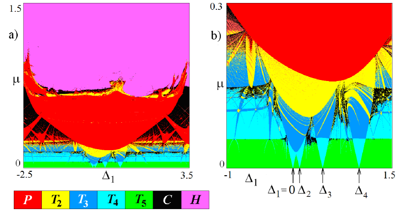
Figure 1: Chart of Lyapunov exponents for the network of five phase oscillators (3) and its enlarged fragment for $\Delta_{2}=0.1,\Delta_{3}=0.45$, $\Delta_{4}=1$.

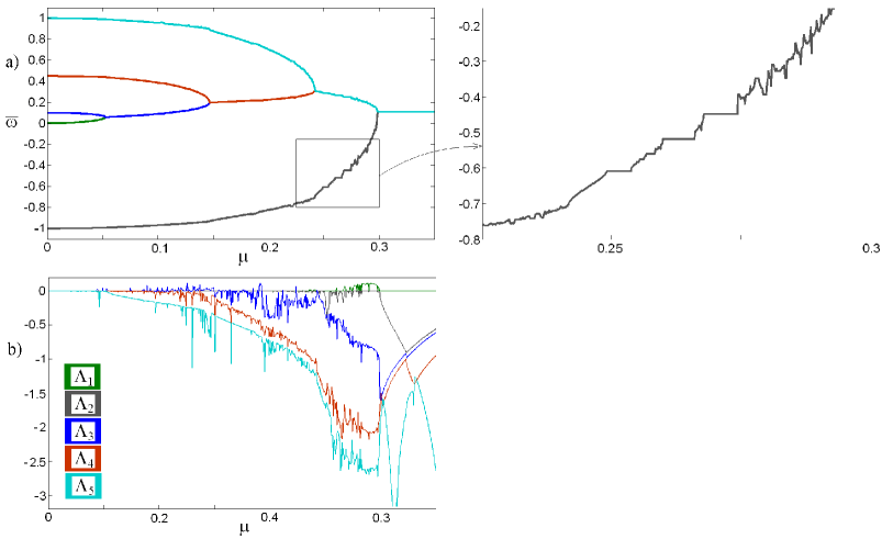
Figure 2: (a) Synchronization tree and its enlarged fragment (right) illustrating complicated structure of this tree. (b) Plot of Lyaponov exponents for the network of five discrete phase oscillators (3). Values of the parameters are $\Delta_{1}=-1$, $\Delta_{2}=0.1,\Delta_{3}=0.45$.

Fig. 2a shows the dependence of frequencies $\bar{\omega}_{i}={\mathop{\lim}\limits_{n\to\infty}}{\frac{{\psi_{i}^{(n)}-\psi_{i}^{(0)}}}{{n}}}$ which are observed in the system on coupling value. Consider the case $\Delta_{1}=-1$ (left border in Fig. 1b). When $\mu=0$, the observed frequencies are equal to the natural frequencies of the oscillators, i.e., according to (3):

$$\bar{\omega}_{1}=0{\rm,}\quad\bar{\omega}_{2}=\Delta_{1}{\rm,}\quad\bar{\omega}_{3}=\Delta_{2}{\rm,}\quad\bar{\omega}_{4}=\Delta_{3}{\rm,}\quad\bar{\omega}_{5}=\Delta_{4}.$$ (4)

In Fig. 2a one can see a sequential emergence of clusters which corresponds to the consecutive merging of the “tree branches”. For example, the first cluster arises when the first and the second oscillators join together. After this, the third one is joined to them, and etc. It should be noted that the number of clusters does not strictly correspond to the dimension of the observed torus. A plot of Lyapunov exponents in Fig. 2b verifies this fact. An enlarged fragment of the tree in Fig. 2a (right) shows that the tree branch is jagged in the domain where there is multiple alternation of two-frequency, periodic and chaotic regimes.

Now discuss structure of the parameter plane given in Fig. 1. Consider the domain of small coupling values. One can see that the five-frequency tori are dominant. However, there are several tongues of the four-frequency regimes. At the bottom, they look like traditional Arnol’d tongues. At some points they touch the $\Delta_{1}$-axis. We can derive coordinates of these points using physical consideration. Variation of the frequency $\omega{}_{1}$ leads to the consistent resonances between the second oscillator and the first, third, fourth and fifth one. From the definition of frequency detunings $\Delta_{i-1}=\omega_{i}-\omega{}_{1}$, we obtain four resonance conditions

$$\Delta_{1}=0{\rm,}\quad\Delta_{1}=\Delta_{2}{\rm,}\quad\Delta_{1}=\Delta_{3}{\rm,}\quad\Delta_{1}=\Delta_{4}{\rm.}$$ (5)

These values are indicated by vertical arrows in Fig. 1b.

We choose the spectrum of oscillators so that the frequencies of the fourth oscillator and the fifth one are sufficiently different. Thus, the two right-hand tongues in Fig. 1b satisfying the conditions $\omega_{4}\approx\omega{}_{1}$ and $\omega_{5}\approx\omega{}_{1}$ have a very simple structure. They represent two domains of four-frequency tori inside the five-frequency one. In these cases, the second oscillator is in resonance with only one oscillator, and the other ones are actually independent. This is a kind of the “individual” resonance.

At the same time, frequencies of the first and the third oscillators are nearly equal: $\omega_{1}\approx\omega{}_{3}$ ($\Delta_{2}\approx 0$). Therefore, the second test oscillator interacts with this pair at the variation of its frequency $\Delta_{1}$. This is a kind of the “collective” resonance. In such a case synchronization picture is more complicated and is shown in detail in Fig. 3a. One can see that the four-frequency tongues are closed by edges forming a characteristic oval domain of three-frequency tori $T_{3}$. In this case, a cluster of three oscillators (the first, second and third ones) may arise.

At the same time, inside the five-frequency domain $T_{5}$ there are many thin higher-order tongues of four-frequency tori. Fig. 3b illustrates two types of them. In the first case, the tongue has a traditional cusp shape. In the second case, a fan-shaped system of four-frequency tori is located at the bottom of the rounded three-frequency domain. Small chaotic regions may also be observed.

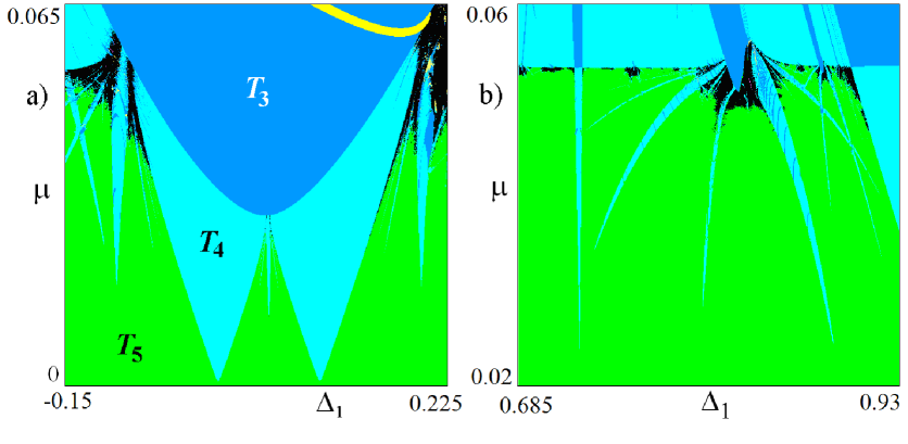
Figure 3: (a) Integration of the four-frequency tongues. (b) Two higher-order tongues of four-frequency tori. The colour palette is similar to that in Fig. 1.

With an increase in the coupling parameter ($\mu\geq 0.05$), the five-frequency regimes in Fig. 1 are replaced by the four-frequency regimes. The corresponding boundary looks like a horizontal line. It is a saddle-node bifurcation line for the four-frequency torus. Above this line, there is a characteristic picture of the Arnol’d resonance web [19] which is shown in Fig. 4a. In this case, there is a network of three-frequency domains with dual-frequency regimes arising at their regions of intersection. It should be noted that this result is somewhat unexpected. The resonance web arises usually on the parameter plane of the fundamental frequencies of the oscillators [18, 19]. In our case, one of the parameters is the coupling. We can give following explanation of this fact. The oscillation frequency for the arising cluster depends on the coupling value. Thus, the resonance conditions occur with simultaneous variation of the frequency and the coupling. Note that with an increase in coupling $\mu$ the resonance web structure remains in Fig. 4a, but the four-frequency regimes are replaced by the chaotic ones.

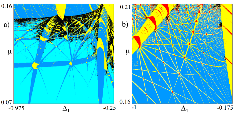
Figure 4: Resonance web for the network of five discrete phase oscillators (3) inside the domain of (a) four-frequency and (b) five-frequency tori.

For $\mu\geq 0.15$, the three-frequency region is observed. In this case, there is also a resonance web, but it is on the basis of the three-frequency regimes as is shown in Fig. 4b.

For larger values of $\mu$, there is a domain of two-frequency quasiperiodic regimes which looks like a band (Fig. 5a). There is also a system of higher-order complete resonances. They look like the traditional Arnol’d tongues, but with the destroyed bottoms. One can see diverse kinds of the complete resonances on the chart of periodic regimes in Fig. 5b. In this case, the different colours indicate different periods of cycles of the analyzed map. Near the bottom of each tongue of periodic regimes, the system of fan-shaped domains of two-frequency tori arises. Inside the tongues of periodic regimes, there is a period doubling which leads to chaos with an increase in the coupling parameter.

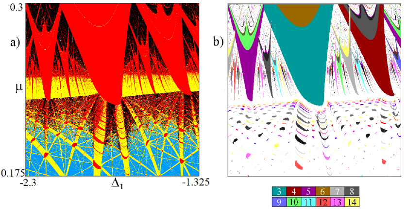
Figure 5: Higher-order tongues of the complete synchronization embedded in the quasiperiodic domains of different dimension and chaos. (a) Chart of Lyapunov exponents; (b) chart of periodic regimes; numbers below indicate periods of cycles.

3 Comparison with the dynamics of the chain of oscillators

Now discuss an influence of the coupling geometry in the system to the synchronization. For this purpose, we compare the above results with the results for oscillators coupled in a linear chain. In this case, the phase equations are

$$\begin{array}[]{l}\psi_{1}\to\omega{}_{1}+\psi_{1}+\mu\sin(\psi_{2}-\psi_{1}),\\ \psi_{2}\to\omega_{2}+\psi_{2}+\mu{\left[{\sin(\psi_{1}-\psi_{2})+\sin(\psi_{3}-\psi_{2})}\right]},\\ \psi_{3}\to\omega_{3}+\psi_{3}+\mu{\left[{\sin(\psi{}_{2}-\psi_{3})+\sin(\psi_{4}-\psi_{3})}\right]},\\ \psi_{4}\to\omega_{4}+\psi{}_{4}+\mu{\left[{\sin(\psi_{3}-\psi_{4})+\sin(\psi_{5}-\psi_{4})}\right]},\\ \psi_{5}\to\omega_{5}+\psi_{5}+\mu\sin(\psi_{4}-\psi_{5}).\\ \end{array}$$ (6)

For the relative phases (2), we obtain the following system of equations:

$$\begin{array}[]{l}\theta\to\theta+\Delta_{1}+\mu(-2\sin\theta+\sin\varphi),\\ \varphi\to\varphi+\Delta_{2}-\Delta_{1}+\mu(-2\sin\varphi+\sin\theta+\sin\alpha),\\ \alpha\to\alpha+\Delta_{3}-\Delta_{2}+\mu(-2\sin\alpha+\sin\beta+\sin\varphi),\\ \beta\to\beta+\Delta_{4}-\Delta_{3}+\mu(-2\sin\beta+\sin\alpha).\\ \end{array}$$ (7)

Fig. 6 shows the corresponding chart of Lyapunov exponents constructed for the same values of the parameters as in Fig. 1. In this case, the number of basic resonance tongues of four-frequency tori reduces from four to two. This has a physical explanation. Indeed, variation of the frequency for the second oscillator $\omega_{2}$ may lead to one of the two possible resonances $\omega_{2}=\omega_{1}$, $\omega_{2}=\omega_{3}$due to the coupling geometry in the chain. This provides the conditions

$$\Delta_{1}=0{\rm,}\quad\Delta_{1}=\Delta_{2}{\rm.}$$ (8)

Thus, we obtain an interesting result: the number of basic tongues of four-frequency tori equals to the number of nearest neighbors of the oscillator with a variable frequency. It will also be true for networks with a more complex coupling topology.

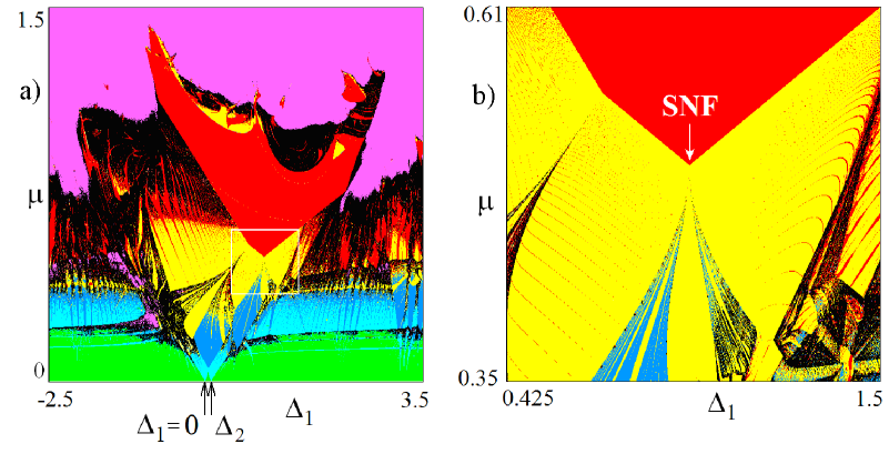
Figure 6: (a) Chart of Lyapunov exponents for the chain of five phase oscillators (7) and (b) its enlarged fragment. Values of the parameters are $\Delta_{2}=0.1,\Delta_{3}=0.45$, $\Delta_{4}=1$. SNF is saddle-node fan point [18, 20].

Another conclusion is that the shape of the complete synchronization domain for the network and for the chain of oscillators is different (compare Fig. 1b and Fig. 6b). In the last case, there are characteristic angles corresponding to the codimension-two points (Fig. 6b). These points are typical also for flow models [20].

4 System with anti-phase synchronization

We have considered the dissipative coupling which tends to equalize the states of oscillators. In the simplest case of two elements, this type of coupling leads to the in-phase synchronization. However, the case of negative values of the coupling is also important. In this case, the anti-phase synchronization is stable for two coupled elements. This type of coupling is characteristic, for example, for laser physics when lasers are optically coupled by radiation through the sidewalls of waveguides [22, 23, 24]. It may be called an active coupling or repulsive interaction [25].

Let us discuss the case of an active coupling. Firstly, consider a chain of oscillators. In this case, there is a certain symmetry in the system. Indeed, Eqs. (7) are invariant under a linear change of variables

$$\mu\to-\mu{\rm,}\quad\theta\to\theta+\pi,\quad\varphi\to\varphi+\pi,\quad\alpha\to\alpha+\pi,\quad\beta\to\beta+\pi.$$ (9)

This transformation of variables does not change the type and stability characteristics of fixed points. Only a phase shift of $\pi$ occurs and a change from the in-phase to anti-phase regimes is observed. Therefore, the chart of dynamic regimes for the oscillators with anti-phase synchronization looks exactly like the chart in Fig. 6. Thus, a complete synchronization between all the subsystems is possible in the chain of coupled oscillators.

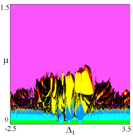
Figure 7: Chart of Lyapunov exponents for the network of five phase oscillators in case of an active coupling for $\Delta_{2}=0.1,\Delta_{3}=0.45,\Delta_{4}=1$.

There is another situation in case of globally coupled elements. In this case, Eqs. (3) are not invariant under the change of variables (8) due to the presence of terms containing the sum of relative phases. Therefore, a structure of the parameter space for the network of such elements differs from that for the chain. Fig. 7 shows the chart of Lyapunov exponents for the oscillators with anti-phase synchronization with the same values of fundamental frequencies as in Fig.1. One can see that for small values of $\mu$, the picture is partly equivalent to the case of the dissipative coupling. Thus, if two or three oscillators are captured inside the network of coupled oscillators, the system behaviour is qualitatively the same for any sign of the coupling parameter. For high values of the coupling, there are great differences between these two situations. An ordered structure of two-frequency quasiperiodic domains, which is typical for the dissipative coupling, is destroyed. A domain of the complete synchronization virtually disappears in case of an active coupling and only a few isolated “islands” of periodic regimes are visible. Thus, the Kuramoto transition does not occur for an active coupling. Instead, the chaotic or even hyperchaotic regimes are observed. This result is important for laser arrays because it means that the coupling configuration of type “each-to-each” is not always a good method to get coherent radiation.

5 Conclusion

Two-parameter Lyapunov analysis is an effective tool for the study of ensembles of discrete phase oscillators. Another useful trick is a frequency scanning of the system properties via using one dedicated oscillator. Features of the dynamics in low-dimensional network ensembles are investigated in case of the five discrete phase oscillators. There are characteristic domains of different-order resonance tori. Bottoms of these domains are destroyed and form the fan-shaped system of domains of higher-order tori. For medium values of the coupling, there is Arnol’d resonance web on the “frequency detuning – coupling” parameter plane. It exists in both the domains of three- and four-frequency tori. The case of synchronization of oscillators with repulsive interaction in the domain of strong coupling is significantly different from the case of in-phase synchronization, in particular, full synchronization modes are atypical.

References

- [1] Pikovsky A., Rosenblum M., Kurths J. Synchronization: a universal concept in nonlinear sciences. Cambridge University Press. 2001.
- [2] Landa P.S. Nonlinear Oscillations and Waves in Dynamical Systems. Kluwer Academic Publishers, Dordrecht. 1996.
- [3] Balanov A.G., Janson N.B., Postnov D.E., Sosnovtseva O. Synchronization: from simple to complex. Springer. 2009.
- [4] Glass L., Mackey M.C. From clocks to chaos: The rhythms of life. Princeton University Press. 1988.
- [5] Kuramoto Y. Chemical Oscillations, Waves and Turbulence. Springer, Berlin. 1984.
- [6] Strogatz S.H. From Kuramoto to Crawford: exploring the onset of synchronization in populations of coupled oscillators // Physica D. 2000. Vol.143. P.1.
- [7] Acebrón J.A., Bonilla L. L., Pérez Vicente C.J., Ritort F., Spigler R. The Kuramoto model: a simple paradigm for synchronization phenomena // Reviews of Modern Physics. 2005. Vol.77, P.137.
- [8] Maistrenko Yu., Popovych O., Burylko O., Tass P.A. Mechanism of desynchronization in the finite-dimensional Kuramoto model // Phys. Rev. Lett. 2004. Vol.93, 084102.
- [9] Zaslavsky G. M. The Physics of Chaos in Hamiltonian Systems. London: Imperial College Press, 2007.
- [10] Khoshsiar Ghaziani R., Govaerts W., Sonck C. Codimension-two bifurcations of fixed points in a class of discrete prey-predator systems // Discrete Dynamics in Nature and Society. 2011. Article ID 862494.
- [11] Han W., Liu M. Stability and bifurcation analysis for a discrete-time model of Lotka–Volterra type with delay // Applied Mathematics and Computation. 2011. Vol. 217. P. 5449.
- [12] de Souza S.L.T., Lima A.A., Caldas I.L., Medrano-T. R.O., Guimarães-Filho Z.O. Self-similarities of periodic structures for a discrete model of a two-gene system // Phys. Lett. A. 2012. Vol. 376. P. 1290.
- [13] Andrecut M., Kauffman S.A. Chaos in a discrete model of a two-gene system // Phys. Lett. A. 2007. Vol. 367. P.281.
- [14] Arrowsmith D.K., Cartwright J.H.E., Lansbury A.N., Place C.M. The Bogdanov map: bifurcations, mode locking, and chaos in a dissipative system // Int. J. Bifurcation Chaos. 1993. Vol.3. P. 803.
- [15] Barlev G., Girvan M., Ott E. Map model for synchronization of systems of many coupled oscillators // CHAOS. 2010. Vol.20. 023109.
- [16] Vasylenko A., Maistrenko Yu., Hasler M. Modelling the phase synchronization in systems of two and three coupled oscillators // Nonlinear Oscillations. 2004. Vol.7. P.311.
- [17] Maistrenko V., Vasylenko A., Maistrenko Yu., Mosekilde E. Phase chaos in the discrete Kuramoto model // Int. J. Bifurcation Chaos. 2010. Vol. 20. P.1811.
- [18] Baesens C., Guckenheimer J., Kim S., MacKay R.S. Three coupled oscillators: mode locking, global bifurcations and toroidal chaos // Physica D. 1991. Vol.49. P.387.
- [19] Broer H.W., Simó C., Vitolo R. The Hopf-saddle-node bifurcation for fixed points of 3D-diffeomorphisms: the Arnol’d resonance web // Bull. Belg. Math. Soc. Simon Stevin. 2008. Vol.15. P.769.
- [20] Emelianova Yu.P., Kuznetsov A.P., Sataev I.R., Turukina L.V. Synchronization and multi-frequency oscillations in the low-dimensional chain of the self-oscillators // Physica D. 2013. Vol.244. P.36.
- [21] Kuznetsov A.P., Sataev I.R., Turukina L.V. On the road towards multidimensional tori // Commun Nonlinear Sci Numer Simul. 2011. Vol.16. P.2371.
- [22] Khibnik A.I., Braiman Y., Kennedy T.A.B., Wiesenfeld K. Phase model analysis of two lasers with injected field // Physica D. 1998. Vol. 111. P 295.
- [23] Glova A. F., Lysikov A. Yu. Phase locking of three lasers optically coupled with a spatial filter // Quantum Electronics. 2002. Vol.32. P.315.
- [24] Glova A. F. Phase locking of optically coupled lasers // Quantum Electronics. 2003. Vol.33. P.283.
- [25] Hong H., Strogatz S.H. Mean-field behavior in coupled oscillators with attractive and repulsive interactions // Phys. Rev. E. 2012. Vol.85. 056210[6 pages].
- [26] Anishchenko V., Astakhov S., Vadivasova T. Phase dynamics of two coupled oscillators under external periodic force // Europhys. Lett. 2009. Vol. 86. P.30003.
- [27] de Lima M.R., Claro F. , Ribeiro W., Xavier S., López-Castillo A. The numerical connection between map and its differential equation: logistic and other systems // Int. J. Nonlinear Sci. Numer. Simul. 2013. Vol. 14. P.77.