Revision of the brick wall method for calculating the black hole thermodynamic quantities

Abstract

Within the framework of the “brick wall model”, a novel method is developed to compute the contributions of a scalar field to the thermodynamic quantities of black holes. The relations between (transverse) momenta and frequencies in Rindler space are determined numerically with high accuracy and analytically with an accuracy of better than 10 % and are compared with the corresponding quantities in Minkowski space. In conflict with earlier results, the thermodynamic properties of black holes turn out to be those of a low temperature system. The resulting discrepancy for partition function and entropy by two orders of magnitude is analyzed in detail. In the final part we carry out the analogous studies for scalar fields in de Sitter space and thereby confirm that our method applies also to the important case of spherically symmetric spaces.

I Introduction

The relations between momenta and energies are fundamental quantities in statistical physics. They determine the density of states and therefore the partition function and other thermodynamic quantities. Similarly, the momentum-frequency relations (“m-f relations”) of fields in the presence of a Killing horizon determine the corresponding thermodynamic quantities. Before calculating them, singularities of the fields at the horizon have to be regularized. We adopt the most commonly used “brick wall” method tHOO85 ; SUUG94 ; tHOO96 which regularizes these singularities by restricting the fields to a region close to but outside the horizon. Within this framework a variety of investigations (cf. MUIS98 or the reviews FRFU98 , PADM05 where also other approaches are discussed) have been carried out and corrections to the semiclassical approximation have been investigated, cf. SSSS08 , KIKU13 . Other methods have been applied and related to the brick wall method such as the regularization via a Pauli-Villars method DELM95 . In the most commonly applied procedure, the density of states of massless fields is evaluated in a modified WKB approximation where in addition it is assumed that the summation over the modes can be replaced by an integration. To the best of our knowledge, the validity of these approximations has never been verified. It will be analyzed in detail.

We will apply the brick wall model for scalar fields in Rindler space-time. However we will neither assume a priori that the WKB approximation is appropriate nor that the discrete set of eigenvalues can be replaced by a continuum. We will present “exact” numerical results for the m-f relations and the horizon induced partition function and entropy. To provide insight we also will present various approximate, analytical results which together cover the whole range of frequencies. We will show that in the WKB approximation the numerically determined value of the partition function is underestimated by a factor of 3. It is overestimated by two orders of magnitude if the sum over the discrete modes is replaced by an integral which can be determined analytically. It will be seen that the partition function is, up to 1 %, given by the lowest frequency mode. The source of this large discrepancy will be identified and its consequences will be discussed. We also will show that finite mass effects are visible only under extreme conditions.

In order to demonstrate the validity of our method applied to spherically symmetric spaces we have chosen to calculate the thermodynamic quantities of scalar fields in de Sitter space (in the static metric) where not only numerical but again also approximate analytical results can be obtained. We will establish the connection between the angular momentum-frequency relations (“am-f relations”) of de Sitter space and the m-f relations of Rindler space cf. PADM86 .

II Momentum-frequency relations of scalar fields in Rindler space

Scalar Fields in Rindler Space A uniformly accelerated observer in Minkowski space moves along the hyperbola RIND01

$$x^{2}-t^{2}=\frac{1}{a^{2}}\,,\quad{\bf x}_{\perp}=0\,,$$

with the acceleration denoted by $a$ and the coordinates transverse to the motion by ${\bf x}_{\perp}$. After the coordinate transformation

$$t,x,{\bf x}_{\perp}\to\tau,\xi,{\bf x}_{\perp}:\quad t(\tau,\xi)=\frac{1}{a}\;e^{a\xi}\sinh a\tau\,,\quad x(\tau,\xi)=\frac{1}{a}\;e^{a\xi}\cosh a\tau\,,$$ (1)

a particle at rest in the observer’s system at $\xi=\xi_{0}$ corresponds to the uniformly accelerated motion in Minkowski space with acceleration $ae^{-a\xi_{0}}$. The space-time defined by Eq. (1) is the Rindler space with the metric

$$ds^{2}=e^{2\kappa\xi}(d\tau^{2}-d\xi^{2})-d{\bf x}^{2}_{\perp}\,,\quad\kappa=a\,,$$ (2)

where the identity of the acceleration $a$ and the surface gravity $\kappa$ has been used, cf. WALD94 . The coordinate transformation (1) is not one-to-one. The coordinates $-\infty<\tau,\xi<\infty$ cover only one quarter of the Minkowski space, the “Rindler wedge”$R_{+}$

$$R_{\pm}=\big{\{}x^{\mu}\big{|}\,|t|\leq\pm x\big{\}}\,.$$

Upon reversion of the sign of $x$ in Eq. (1) it is the Rindler wedge $R_{-}$ which is covered by the corresponding parametrization. No causal connection exists between the two Rindler wedges $R_{\pm}$.

We consider a non-interacting scalar field $\phi$ in Rindler space with the action

$$S=\frac{1}{2}\int d\tau\,d\xi\,d{\bf x}_{\perp}\big{\{}(\partial_{\tau}\phi)^{2}-(\partial_{\xi}\phi)^{2}-(m^{2}\phi^{2}+(\boldsymbol{\nabla}_{\perp}\phi)^{2}\big{)}\;e^{2\kappa\xi}\big{\}}\,,$$ (3)

which is nothing else than the Minkowski space action restricted to one of its quarters. The solutions of the equations of motion, vanishing exponentially with $\xi\to\infty$, read

$$\phi(\tau,\xi,{\bf x}_{\perp})=e^{-i\omega\tau}e^{i{\bf k}_{\perp}{\bf x}_{\perp}}\,K_{i\omega/\kappa}\big{(}z(\xi)\big{)}\,,\quad z(\xi)=\frac{1}{\kappa}\sqrt{m^{2}+k_{\perp}^{2}}\,e^{\kappa\xi}\,,$$ (4)

with the MacDonald function satisfying the differential equation

$$\big{[}-\frac{d^{2}}{d\xi^{2}}+(m^{2}+k_{\perp}^{2})\,e^{2\xi}-\omega^{2}\big{]}K_{i\omega/\kappa}(z(\xi))=0.$$ (5)

Here and in the following we assume dimensionful quantities to be given in units of powers of $\kappa$. Partition functions and momentum-frequency relations For calculating the thermodynamic quantities, we follow the procedure in SUUG94 and restrict the system under consideration to a part of the Rindler space. The resulting discrete spectrum consists of eigenvalues characterized by 3 integers $n,n_{2},n_{3}$ and the basic thermodynamic quantity, the partition function, is given by,

$$\ln Z=-\sum_{n,n_{2},n_{3}}^{\infty}\ln\big{(}1-e^{-\beta\,\omega(n,n_{2},n_{3})}\big{)}\,.$$ (6)

In the transverse directions the system is restricted to a square with side-length $\mathcal{L}$. We impose periodic boundary conditions and replace the sum over $n_{2},n_{3}$ by an integral,

$$\ln Z=-\frac{{\mathcal{A}}}{2\pi}\sum_{n=1}^{\infty}\int_{0}^{\infty}k_{\perp}\,dk_{\perp}\ln\big{(}1-e^{-\beta\,\omega_{n}(k_{\perp})}\big{)}\,,\quad{\mathcal{A}}={\mathcal{L}}^{2}\,.$$ (7)

The restriction of the $\xi$ variable has to account for the infinite degeneracy of the spectrum LOY08 . Related to this degeneracy is the well known fact that the Minkowski ground state is seen by a uniformly accelerated observer as a system at finite temperature, the (Unruh) temperature, cf. UNRU76 ,

$$T=\frac{1}{\beta}=\frac{1}{2\pi}\,.$$ (8)

Various possibilities exist to remove the degeneracy. We also follow here the procedure in SUUG94 and remove the degeneracy by requiring the space to be limited to the region $\xi\geq\xi_{0}$. We impose Dirichlet boundary conditions for the eigenmodes at the finite distance $e^{\xi_{0}}$ from the horizon. Due to the exponential increase of the repulsive “potential” in the wave equation (5), a discrete spectrum with respect to the $\xi$ variable is obtained without erecting a second wall. For a given value of $\omega$ and given the number $n$ of zeroes, the vanishing of the MacDonald function, cf. Eq.(4), determines the value of $k_{\perp}$,

$$K_{i\omega}(\mathcal{K}_{n}(\omega))=0\,,\quad\text{with}\quad\mathcal{K}_{n}(\omega)=e^{\xi_{0}}\sqrt{k_{\perp}^{2}(n,\omega)+m^{2}}\,.$$ (9)

For evaluation of the thermodynamic quantities the level density (cf. Eq. (7)) associated with the transverse motion has to be computed. We shall refer to the resulting relation between ${\mathcal{K}}_{n}$ and $\omega$ as “momentum-frequency (m-f) relation” (cf. the corresponding well known m-f relation (14) in Minkowski space). In terms of these quantities the level density can be computed for any value of the parameters $\xi_{0},\,\mathcal{A},\,m$,

$$\frac{\mathcal{A}}{2\pi}\sum_{n=1}^{\infty}k_{\perp}(n,\omega)dk_{\perp}(n,\omega)=\frac{{\mathcal{A}}}{2\pi\ell^{2}}\sum_{n=1}^{\infty}{\mathcal{K}}_{n}(\omega)\frac{d{\mathcal{K}}_{n}(\omega)}{d\omega}\theta\big{(}{\mathcal{K}}_{n}(\omega)-m_{\ell}\big{)}\,d\omega\,,$$ (10)

where $\ell=e^{\xi_{0}}$ denotes the distance of the boundary to the horizon and $m_{\ell}$ the mass of the field in units of $1/\ell$. According to Eq. (7) the logarithm of the partition function reads

$$\ln Z=\frac{\mathcal{A}}{4\ell^{2}}\,\sum_{n=1}^{\infty}\zeta_{n}(\beta,\omega_{n}^{0})\,,$$ (11)

where, after an integration by parts, the functions $\zeta_{n}$ are given by,

$$\zeta_{n}(\beta,\omega_{n}^{0})=\frac{1}{\pi}\Big{(}{\mathcal{K}}_{n}^{2}(\omega_{n}^{0})\ln\big{(}1-e^{-\beta\omega_{n}^{0}})+\beta\int_{\omega_{n}^{0}}^{\infty}d\omega\,\Phi_{n}(\omega,\beta)\Big{)}\,,\quad\Phi_{n}(\omega,\beta)=\frac{{\mathcal{K}}_{n}^{2}(\omega)}{e^{\beta\omega}-1}\,,$$ (12)

with the lower limit of the $\omega$-integration (cf. Eq. (9)),

$${\mathcal{K}}_{n}(\omega_{n}^{0})=m_{\ell}\,.$$ (13)

In the following we assume the mass to vanish. It will be shown in the last paragraph of Section III that only under extreme conditions finite mass effects can become relevant. m-f relations in Rindler and Minkowski space The m-f relations and partition function in Rindler space will be compared in the following with the corresponding quantities in Minkowski space. To this end, we assume a scalar massless field to be confined in one direction to an interval of size $\lambda$, i.e., the Minkowski space m-f relations are given by, (for comparison, cf. Eq. (9)),

$$\mathcal{K}_{M,n}(\omega)=\sqrt{\omega^{2}-\big{(}n\pi/\lambda\big{)}^{2}}\,,$$ (14)

and the partition function reads (cf. Eq. (7) and for comparison Eqs. (11, 12))

$$\hskip 113.81102pt\ln Z_{M}=\frac{\mathcal{A}}{4\lambda^{2}}\sum_{n=1}^{\infty}\zeta_{M,n}(\beta,\lambda),$$

$$\quad\text{with}\quad\zeta_{M,n}(\beta,\lambda)=\frac{\beta\lambda^{2}}{\pi}\int_{n\pi/\lambda}^{\infty}\hskip-8.5359pt\,d\omega\,\Phi_{M,n}(\omega,\beta),\;\;\Phi_{M,n}(\omega,\beta)=\frac{\mathcal{K}_{M,n}^{2}(\omega)}{e^{\beta\omega}-1}\,.$$ (15)

The core of our numerical studies of the m-f relations are displayed in Fig. 1. In a log-log plot are shown the m-f relations in Rindler (${\mathcal{K}}_{n}(\omega)$) and in Minkowski space (${\mathcal{K}}_{M,n}(\omega)$) for various values of $n$. While the Minkowski space m-f relations are given analytically by Eq. (14) the Rindler space m-f relations have been obtained by solving Eq. (9) numerically.

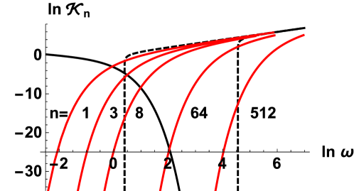
Figure 1: Double logarithmic plots of numerically determined momentum-frequency relations ${\mathcal{K}}_{n}(\omega)$ (Eq. (9)) in Rindler space for five values of $n$ (solid, red curves) are compared with m-f relations (Eq.(14)) in Minkowski space (dashed, black curves) with $\lambda=2.1$ and $n=1$ and $64$. The curve decreasing with $\ln\omega$ is half the logarithm of the “Boltzmann factor” $-0.5\,\ln(e^{\beta\omega}-1),$ cf. Eq. (12) (solid black curve).

Also shown is the square root of the “Boltzmann factor” which, if multiplied with ${\mathcal{K}}_{n}(\omega)$, yields the square root of the integrands of the partition function, cf. Eq. (12). The peculiarities of the Rindler space m-f relations are evident in the comparison with the Minkowski m-f relations. In Minkowski space each of the momenta $\mathcal{K}_{M,n}$ exhibits a threshold which for vanishing mass is given by $\omega=n\pi/\lambda$ (cf. Eq.(14)) while in Rindler space the m-f relations cover the whole range of $\omega$. This is a consequence of imposing in Rindler space only one boundary condition (cf. Eq.(9)). Unlike in Minkowski space, a second boundary condition is not necessary due to the infinitely increasing strength of the repulsion (cf. Eq.(5)) with increasing $\xi$. In other words, the waves “tunnel” into a region which for instance would not be accessible to a classical particle.

For assessing the accuracy of the numerically determined zeroes of the MacDonald functions, cf. Eq. (9), a well defined measure is the following quantity, cf.RG65 ,

$$\chi(\omega,n)=\frac{K_{i\omega}(z)}{z\frac{d}{dz}K_{i\omega}(z)}=\frac{K_{i\omega-1}(z)-K_{i\omega+1}(z)}{i\omega(K_{i\omega-1}(z)+K_{i\omega+1}(z))}\,.$$

For $-2.4\leq\ln\omega\leq 6.0$ (cf. Fig. 1), and for $n=1$ (with similar results for $n>1$) the accuracy varies in the interval,

$$-42\leq\ln\chi(\omega,1)\leq-32\,.$$

Having determined the m-f relations one can proceed directly to Section III and determine by integrations the thermodynamic quantities. Before proceeding however, we will develop two different but complementary analytical approximations, the “pole dominance” (PD) and the WKB approximation in order to gain insight into the properties of the m-f relations. Pole dominance approximation In the small ${\mathcal{K}}_{n}/\omega$ regime, the m-f relations are determined by the asymptotics, $\xi_{0}\ll-1,$ of the MacDonald functions, cf. RG65 ,

$$k_{i\omega}({\mathcal{K}}_{n})\approx-\sqrt{\frac{2}{\pi}}\;\sin\big{(}\omega\xi_{0}-\delta\big{)}\,,\quad e^{2i\delta}=\frac{\Gamma(1+i\omega)}{\Gamma(1-i\omega)}\left(\frac{e^{-\xi_{0}}{\mathcal{K}}_{n}(\omega)}{2}\right)^{-2i\omega}\,.$$

Thus, $k_{i\omega}({\mathcal{K}}_{n})$ vanishes if $\omega\xi_{0}-\delta+n\pi=0,$ and we obtain,

$$\ln\,{\mathcal{K}}_{n}(\omega)\approx(\arg\Gamma(1+i\omega)-n\pi)/\omega+\ln 2\,\equiv\ln\,\tilde{{\mathcal{K}}}_{n}(\omega).$$ (16)

The positions of the singularities of ${\mathcal{K}}_{n}$ in the complex $\omega$-plane coincide with the positions of the poles of the Rindler space propagator Fourier transformed in time LOY11 , and we shall refer to (16) as pole dominance (“PD”) approximation. The accuracy of this approximation together with the WKB approximation as functions of the logarithm of $\omega$ for various values of $n$ is shown in Fig. 2.

To analyze the shape of the m-f relations we first consider the small $\omega$ region where the m-f relation (16) simplifies,

$$\tilde{{\mathcal{K}}}_{n}\underset{\omega\to 0}{\sim}e^{-(n\pi/\omega+\gamma-\ln 2)}\,,$$ (17)

with Euler’s constant $\gamma$. It exhibits an essential singularity at $\omega=0$ which is responsible for the steep increase of $\tilde{{\mathcal{K}}}_{n}$ with $\omega$. This behavior has its origin in the infinite degeneracy of the spectrum of the Rindler space Hamiltonian in the absence of the boundary (cf. the wave equation (5)) corresponding to a vertical line for each value of $\omega$. Furthermore, as in the degenerate case, in the regime of validity of Eq. (17), the curves for different $n$ are parallel, i.e., for $\tilde{{\mathcal{K}}}_{m}(\omega_{m})=\tilde{{\mathcal{K}}}_{n}(\omega_{n})$ these curves satisfy $\ln\omega_{m}-\ln\omega_{n}=\ln m-\ln n$ . The vertical distances between the curves (cf. Fig. 1) are given by Eq. (16) ,

$$\ln\tilde{{\mathcal{K}}}_{m}(\omega)-\ln\tilde{{\mathcal{K}}}_{n}(\omega)=(n-m)\pi/\omega\,,$$ (18)

in agreement within 10% with the numerical results for $\omega\leq 8$ (cf. Fig. 2). According to Eq. (16), the m-f relations, evaluated in PD approximation, converge to the limit,

$$\tilde{\mathcal{K}}_{n}(\omega)\underset{\omega\to\infty}{\sim}\frac{2\omega}{e}e^{-(n-1/4)\pi/\omega},$$ (19)

which deviates from the numerically determined asymptotics by the factor $2/e$.

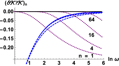
Figure 2: Deviations $\tilde{\mathcal{K}}_{n}/{\mathcal{K}}_{n}-1$ of the pole dominance approximation, decreasing with increasing $\ln\,\omega$, (dotted, purple lines) and of the WKB approximations $\hat{{\mathcal{K}}}_{n}/{\mathcal{K}}_{n}-1$, increasing with increasing $\ln\,\omega$, (dashed, blue lines) from the exact results. Asymptotically, the deviations $\tilde{{\mathcal{K}}}_{n}(\omega)/{\mathcal{K}}_{n}(\omega)-1$ approach the $\ln\omega$-axis $\delta\mathcal{K}/\mathcal{K}=2/e-1$, cf. Eq. (19) and the deviations $\hat{{\mathcal{K}}}_{n}(\omega)/{\mathcal{K}}_{n}(\omega)-1$ approach 0, cf. Fig. 1 and Eq. (23). For fixed $\omega$ the absolute values of the deviations (of pole dominance and WKB approximations) decrease with increasing $n$.

WKB approximation For not too small values of $\omega$ (cf. Fig. 2), the WKB approximation  tHOO85 , can be applied successfully for calculating the m-f relations. Together with an additional approximation, it has become the most common tool for calculating analytically thermodynamic quantities in Schwarzschild tHOO85 and Rindler SUUG94 spaces (cf. also the reviews FRFU98 and PADM05 ). The WKB m-f relations, $\hat{{\mathcal{K}}}_{n}(\omega)$,  are obtained by solving the equation, cf. SUUG94 , tHOO85 ,

$$n\pi=\int_{\xi_{0}}^{\xi_{1}}d\xi\sqrt{\omega^{2}-e^{2(\xi-\xi_{0})}\hat{{\mathcal{K}}}^{2}_{n}(\omega)}\,,$$ (20)

where $\xi_{1}$ denotes the turning point. This integral can be evaluated analytically and the WKB m-f relations are obtained as solutions of the following equation,

$$\frac{n\pi}{\omega}=h(\eta)\,,\quad h(\eta)=-\sqrt{1-\eta^{2}}+\ln\big{(}\sqrt{1-\eta^{2}}+1\big{)}-\ln\eta\,,\quad 0\leq\eta=\frac{\hat{{\mathcal{K}}}_{n}}{\omega}\leq 1\,.$$ (21)

This equation implies that the solutions $\hat{{\mathcal{K}}}_{n}$ are given in terms of the inverse of the function,

$$\hat{{\mathcal{K}}}_{n}(\omega)=\omega\,h^{-1}\Big{(}\frac{n\pi}{\omega}\Big{)}\,.$$ (22)

Although a complete analytical solution cannot be attained, expansion of $h(\eta)$ around $\eta=0$ and $\eta=1$ yield explicit expressions in the limits of small and of large values of $\omega$ respectively,

$$\hat{{\mathcal{K}}}_{n}(\omega)\underset{\omega\to 0}{\sim}\omega\,e^{-(n\pi/\omega+1-\ln 2)}\,,\quad\quad\hat{{\mathcal{K}}}_{n}(\omega)\underset{\omega\to\infty}{\sim}\omega\Big{(}1+\frac{1}{2}\Big{(}\frac{3n\pi}{\omega}\Big{)}^{2/3}+\frac{7}{40}\Big{(}\frac{3n\pi}{\omega}\Big{)}^{4/3}\Big{)}^{-1}\,.$$ (23)

As one might expect, the semiclassical WKB approximation fails to describe properly the m-f relations in the small $\omega$ limit. Compared to the PD approximation $\tilde{K}_{n}(\omega)$ (17) which becomes exact in the small $\omega$ limit, the corresponding WKB approximation is suppressed (cf. Fig.2) by the factor $\omega\,e^{-1+\gamma}$. It reproduces however, in agreement with the numerical results, the $\omega\to\infty$ limit of the m-f relation.

We observe that for large values of $\omega$ the Rindler and Minkowski space m-f relations still exhibit significant differences. While in Minkowski space, the momenta with different $n$ converge, they diverge in Rindler space (cf. Eq. (23))

$${\mathcal{K}}_{M,n}(\omega)-{\mathcal{K}}_{M,m}(\omega)\enskip\underset{\omega\to\infty}{\longrightarrow}\enskip\frac{1}{2\omega}\frac{\pi^{2}}{\lambda^{2}}(m^{2}-n^{2}),\quad\hat{{\mathcal{K}}}_{n}(\omega)-\hat{{\mathcal{K}}}_{m}(\omega)\enskip\underset{\omega\to\infty}{\longrightarrow}\enskip\frac{(3\pi)}{2}^{2/3}(m^{2/3}-n^{2/3})\,\omega^{1/3}\,.$$

Fig. 1 demonstrates this difference between Rindler and Minkowski space at $\ln\omega\geq 4.6$. Related to this property is the difference of the level density at large $\omega$ (cf. Eq.(14)),

$$\frac{1}{2}\frac{d}{d\omega}\hat{{\mathcal{K}}}_{n}^{2}(\omega)\enskip\underset{\omega\to\infty}{\longrightarrow}\omega-\frac{2}{3}(3n\pi)^{2/3}\omega^{1/3},\qquad\,\frac{1}{2}\frac{d}{d\omega}{\mathcal{K}}_{M,n}^{2}(\omega)=\omega\,.$$ (24)

III Thermodynamic quantities

Thermodynamic properties of massless fields Given the m-f relations, the thermodynamic quantities are, apart from a boundary term, (present only if $m\neq 0$) obtained by integrating ${\mathcal{K}}_{n}^{2}(\omega)$ over $\omega$ weighted with the “Boltzmann factor” (Eq. (12)) and by summing over $n$. The integrands are shown in Fig. 3 for $n=1,2,3$. These curves are the result of the interplay between the increasing squared momenta and the decreasing “Boltzmann factor” as a function of $\omega$ cf. Fig.1. The positions of the maxima coincide roughly with the positions of the crossing of the squared momenta and of the “Boltzmann factor” in Fig.1. These results demonstrate dominance of the $n=1$ contribution which in turn is dominated by the maximum at $\omega\approx 1$ with ${\mathcal{K}}_{1}\approx 0.06$ (cf. Fig. 1). Also shown is the integrand of the corresponding Minkowski space quantity $\Phi_{M,1}(\omega)$ (cf. Eq. (15)) which, due to the presence of threshold at $\omega_{th}=\pi/\lambda=\pi/2.1$ (cf. Fig. (1)), exhibits a rather different structure. The maximum is reached at $\omega\approx\omega_{th}+1/\beta$ and approaches $\Phi_{1}(\omega)$ asymptotically (cf. Eqs. (15), (23))

$$\frac{\Phi_{M,1}(\omega)}{\Phi_{1}(\omega)}\enskip\underset{\omega\to\infty}{\longrightarrow}1+\big{(}3\pi/\omega\big{)}^{2/3}.$$

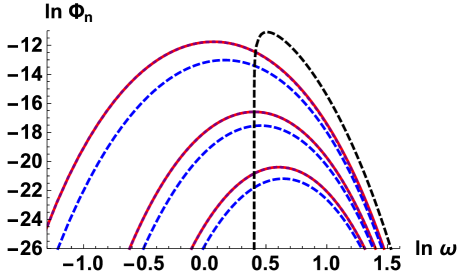
Figure 3: Logarithm of the integrand $\Phi_{n}$ of the partition function (Eq. (12)) as a function of $\ln\omega$ for $n=1,2,3$ , calculated numerically (solid, (red) lines), in the PD approximation (dotted, (purple) lines) and in the WKB approximation (dashed, (blue) lines) in comparison with the Minkowski-space quantity $\ln\Phi_{M,1}(\omega)$ (cf. Eq. (15)).

Given these results for $\Phi_{n}(\omega)$, it is straightforward to determine numerically the logarithm of the partition function (cf. Eqs. (11,12)) and the entropy,

$$S=\frac{{\mathcal{A}}}{4\ell^{2}}(1-\beta\,\partial_{\beta})\sum_{n=1}^{\infty}\zeta_{n}(\beta,\omega_{n}^{0})\Big{|}_{\beta=2\pi},$$ (25)

and to study analytically these quantities. In the PD approximation the $n$-sum can be carried out with the help of the relation (18), and the calculation of the logarithm of the partition function is reduced to a quadrature (cf. Eq. (16)),

$$\ln\tilde{Z}=\frac{\beta\mathcal{A}}{\pi\ell^{2}}\,\int_{0}^{\infty}\,\frac{e^{2\arg\,\Gamma(1+i\omega)/\omega}\,d\omega}{(e^{\beta\omega}-1)(e^{2\pi/\omega}-1)}\,.$$ (26)

Correspondingly, in the WKB approximation, Eq. (22) implies,

$$\hat{{\mathcal{K}}}_{n}(\omega)=n\,\hat{{\mathcal{K}}}_{1}(\omega/n)\,,$$ (27)

and the partition function can be expressed in terms of $\hat{{\mathcal{K}}}_{1}(\omega)$

$$\ln\hat{Z}=\frac{\mathcal{A}}{4\ell^{2}}\int_{0}^{\infty}d\omega\,\hat{\sigma}(\omega),\;\;\text{with}\;\;\hat{\sigma}(\omega)=\frac{\beta}{\pi}\,\hat{{\mathcal{K}}}_{1}^{2}(\omega)\sum_{n=1}^{\infty}\frac{n^{3}}{e^{\beta n\omega}-1}\,\,.$$ (28)

	$\zeta_{1}\;\;\;\quad$	$\sum_{n}\zeta_{n}$	$S\cdot 4\ell^{2}/\mathcal{A}\quad$
NUM	$1.27\cdot 10^{-5}\;$	$1.30\cdot 10^{-5}$	$9.68\cdot 10^{-5}\;\;$
PD	$1.26\cdot 10^{-5}\;$	$1.28\cdot 10^{-5}\;$	$9.64\cdot 10^{-5}\;\;$
WKB	$3.72\cdot 10^{-6}\;$	$3.77\cdot 10^{-6}$	$3.08\cdot 10^{-5}$

Table 1: $n=1$ and summed contributions to the logarithm of the partition function and up to a factor the entropy $S$ (cf. Eq. (25)) for vanishing mass calculated numerically in the PD and WKB approximations.

The results of our studies of the thermodynamic quantities are compiled in Table 1. Up to corrections of about 1%, the $n\,=\,1$ terms of the logarithm of the partion function (and similarly of the entropy) coincide with the $n$-summed results reflecting the strong suppression of $\ln\Phi_{n}$ with increasing $n$ as displayed in Fig. 3. The PD results agree with the corresponding numerically determined “exact” results with an accuracy of better than 1%, cf. Fig. 3, while the WKB results are too small by a factor of about 3. Black holes as low temperature systems Qualitative confirmation of and insights into the numerical results can be obtained by applying the approximate expression (17) according to which

$$\Phi_{n}(\omega,\beta)\approx 4e^{-2\gamma}e^{-2\pi n/\omega-\beta\omega}\,.$$ (29)

We conclude that the maxima of $\Phi_{n}(\omega,\beta)$ are given by

$$\omega_{n}=\sqrt{2\pi n/\beta},\quad n=1,2,\ldots,$$ (30)

implying

$$\ln\frac{\Phi_{n}(\omega_{n},2\pi)}{\Phi_{1}(\omega_{1},2\pi)}=-4\pi(\sqrt{n}-1)=-5.2,\;-9.2\quad\text{for}\quad n=2,3\,.$$

These values of the positions and ratios of the maxima agree well with the numerical results shown in Fig. 3. Furthermore, by carrying out the $\omega$-integration we obtain (cf. Eq. (12)),

$$\frac{\zeta_{n}}{\zeta_{1}}\approx n^{1/4}\,e^{-4\pi(\sqrt{n}-1)}\approx 0.0065,\;0.00013\quad\text{for}\quad n=2,3\,,$$

which, within 10 and 25 %, agree with the corresponding numerical results. The partition function is dominated by the $n=1$ term with

$$\zeta_{1}\approx 2^{5/2}e^{-2\gamma}e^{-4\pi}=6.22\cdot 10^{-6}\,,$$

which agrees within a factor of 2 with the numerical results in Table 1. In the language of thermodynamics, the dominance of the $n=1$ term is to be interpreted as the low temperature limit. Only by a sufficient increase of the temperature $T\gg 1/2\pi$, i.e., by decreasing the slope of the Boltzmann factor in Fig.1, the modes with $n>1$ can contribute significantly. According to Eq. (30), this is the case if the temperature increases by a factor of $(4\pi(\sqrt{n}-1))^{2}$.

This dominance of the $n=1$ contribution is not at all specific for the Rindler space or the other spaces to be considered. For sufficiently large values of $\upsilon=\beta\pi/\lambda$ which is the case for the choice $\lambda=2.1$, (cf. Fig. 1), the Minkowski space partition function is given by (cf. Eq. (15)),

$$\ln Z_{M}\approx\frac{\mathcal{A}}{\lambda^{2}}\sum_{n=1}^{\infty}\frac{\pi(1+n\upsilon)}{2\upsilon^{2}}e^{-n\upsilon}\,,$$ (31)

i.e., the sudden increase of $\Phi_{M,n}(\omega)$ is due to the thresholds at $\nu_{n}=n\pi/\lambda$ and is dominated by $\zeta_{M,1}$. Modified WKB approximation and analytical expressions for partition function and entropy Since the work of ’t Hooft and of Susskind and Uglum a simplified version of the WKB approximation has been the commonly used tool for calculating analytically the black hole thermodynamic quantities. This simplification is valid only if two conditions are satisfied: The sum over the modes in Eq. (28) can be replaced by an integral and the range of this integration can be increased by changing the lower limit of the integration from 1 to 0, i.e. ,

$$\ln\hat{Z}\to\ln\hat{Z}_{apx}=\frac{\beta\mathcal{A}}{4\pi\ell^{2}}\int_{0}^{\infty}d\nu\,\nu^{3}\int_{0}^{\infty}d\omega\frac{1}{e^{\beta\nu\omega}-1}\,\hat{{\mathcal{K}}}_{1}^{2}(\omega)\,.$$ (32)

After carrying out the $\nu$ integration, also the $\omega$ integral can be calculated analytically with the help of Eqs. (21) and (22),

$$\int_{0}^{\infty}\frac{\nu^{3}}{e^{\nu\beta\omega}-1}\,d\nu=\frac{1}{240}\Big{(}\frac{2\pi}{\beta\omega}\Big{)}^{4}\,,\hskip 28.45274pt\int_{0}^{\infty}\,d\omega\frac{\hat{{\mathcal{K}}}^{2}_{1}(\omega)}{\omega^{4}}=-\frac{1}{\pi}\int_{0}^{1}d\eta\,\eta^{2}\,\frac{dh}{d\eta}=\frac{1}{3\pi}\,,$$ (33)

and yields the following well known expression for the logarithm of partition function and entropy,

$$\ln\hat{Z}_{apx}=\frac{{\mathcal{A}}\,/4\ell^{2}}{360\,\pi}\equiv\frac{1}{4}\hat{S}_{apx}\,,$$ (34)

in agreement with the results in tHOO85 , SUUG94 (provided $\ell$ is identified with the Planck length). However they are in disagreement with the WKB results in Table 1 which are smaller by a factor of 235 and 116 for partition function and entropy respectively. The increase of the partition function by two orders of magnitude if the range of $\nu$ is extended from 1 to 0 does not come as a surprise. An increase of similar strength occurs in the increase of $\Phi_{n}$ when decreasing $n$ from 2 to 1 (cf. Fig.3) which in turn has it’s origin in the increase of both, the square of the momentum $\mathcal{K}_{\nu}(\omega)$ and the “Boltzmann factor” $1/(e^{\beta\omega}-1)$ (cf. Fig.1). As shown in the Appendix, the value of $\ln\hat{Z}_{apx}$ (Eq. (34)) is obtained within $0.1\%$ if the $\nu$ integration, (cf. Eq. (32)) is limited to the unphysical region $0\leq\nu\leq 1$.

The same phenomenon occurs if we proceed to calculate the Minkowski space partition function (31) in a similar way and approximate the $n$-sum by an integration with the result,

$$\ln Z_{M,apx}=\frac{{\mathcal{A}}}{\lambda^{2}}\int_{\nu_{0}}^{\infty}d\nu\,\zeta_{\nu}^{\mu}=\frac{{\mathcal{A}}}{\lambda^{2}}\frac{\pi(2/\upsilon+\nu_{0})}{2\upsilon^{2}}e^{-\upsilon\nu_{0}}\,.$$ (35)

With the values $\nu_{0}=0$ and $\nu_{0}=1$, the ratio of the exact (Eq. (31)) and the approximate results are given, for $\upsilon\gg 1$, by

$$\frac{\ln Z_{M,apx}}{\ln Z_{M}}\Big{|}_{\nu_{0}=0}\approx\frac{2}{\upsilon^{2}}e^{\upsilon}\,,\quad\frac{\ln Z_{M,apx}}{\ln Z_{M}}\Big{|}_{\nu_{0}=1}\approx\frac{1}{\upsilon}\,,$$ (36)

i.e., we find the same pattern as above. Also the Minkowski space partition function is overestimated by orders of magnitude if $\nu_{0}=0$ and much closer to the exact results if $\nu_{0}=1$.

Qualitatively, the failure of replacing the sum over either the Rindler or the Minkowski space modes, by an integration is evident in view of Fig. 1. Only if, as a function of $\omega$, the “Boltzmann factor” is significantly flatter the replacement of the summation by an integration can be justified. In turn, this can be achieved only by increasing the temperature, i.e., by decreasing $\beta$ significantly which however is not an option for the black hole thermodynamics where $\beta=2\pi$. The role of the boundary condition. In concluding our discussion of the thermodynamic quantities of massless fields, we discuss the role of the boundary condition for the thermodynamic quantities. We have seen that the only way to vary the thermodynamic quantities is via the prefactor $\mathcal{A}/4\ell^{2}$. As will be shown in section IV, the expressions for the thermodynamic quantities apply also for de Sitter space and more generally for spherically symmetric spaces with static metrics. The only freedom which is left is the choice of the boundary condition. While irrelevant, cf. FRFU98 , if many modes contribute, the choice of the boundary condition becomes important if only one or a few modes dominate. We demonstrate this uncertainty by modifying the brick wall model and replace the Dirichlet (Eq. (9)) by the Neumann boundary condition which in PD amounts to replace in Eq. (16) $n\pi/\omega\to(n-1/2)\pi/\omega$ resulting in the following expression for the partition function,

$$\ln\tilde{Z}_{Ne}=\frac{\beta\mathcal{A}}{\pi\ell^{2}}\,\int_{0}^{\infty}\,\frac{e^{(2\arg\,\Gamma(1+i\omega)+\pi)/\omega}\,d\omega}{(e^{\beta\omega}-1)(e^{2\pi/\omega}-1)}\,.$$ (37)

Numerical evaluation of this expression yields, in comparison with the results (PD) of Table 1 an enhancement of the partition function by a factor of 32 and of the entropy by a factor of 22. Taking into account that the numerical and the PD values of partition function and entropy are larger than the WKB results (cf. Table 1) by factors of 3.4 and 3.1 respectively, we find that up to factors of 2.1 and 1.7 the values of Eq. (34) are obtained by imposing Neumann boundary conditions, cf. Eq. (37). Effects of masses on thermodynamic properties With introduction of a mass, a new scale enters, (for a calculation of the free energy for massive fields within the WKB approximation cf. KAST94 ). The distance $\ell=e^{\xi_{0}}$ to the horizon appears not only as prefactor $\ell^{-2}$ in the partition function. According to Eq. (12) the thermodynamic properties of both massive and massless fields are determined by the same quantities, ${\mathcal{K}}_{n}(\omega)$. Differences result exclusively from the surface terms, $\sim{\mathcal{K}}_{n}^{2}$, and the presence of the non-vanishing lower limit $\omega_{n}^{0}$ in the $\omega$ integration which is determined by $m_{\ell}$, the product of the mass and the distance to the horizon, cf. Eq. (13). As indicated by Fig. 3, the effect of the non-vanishing surface term and of the lower limit of integration for $n=1$ is, at the level of 1% or smaller, negligible for $\omega\leq 0.5$. Therefore the minimal mass, necessary for affecting the thermodynamic quantities, must satisfy (cf. Eq. (13)),

$$m\geq{\mathcal{K}}_{1}(0.5)\,\,\ell^{-1}\,=2\pi\,{\mathcal{K}}_{1}(0.5)\,T_{\ell}\,,$$

where $T_{\ell}$ denotes the Tolman temperature at the distance $\ell$ from the horizon. Identifying $\ell$ with the Planck length the above inequality reads in terms of the Planck mass $M_{P}$

$$m\geq 2\cdot 10^{-3}M_{P}\,.$$ (38)

Thus unless there are particles with masses of the order of at least $10^{-3}\,\times$ the Planck mass (“Micro black holes”), or there is a reason to increase the distance of the boundary to the horizon from the Planck length to at least $10^{-3}\times$ Compton wavelength of the corresponding particle, the mass of the particle does not affect the thermodynamic quantities.

Given the independence of the thermodynamic quantities from the mass of the particles outside the range (38) we can get a rough estimate of the entropy generated by the particles of the standard model. To this end, we assume that, apart from the multiplicity, all fundamental particles (leptons, quarks, gauge bosons and the Higgs particle) contribute the same amount to the entropy resulting in a value of $s(0)$ (cf. Table 1) of the order of $10^{-2}$. The ambiguity in the choice of the boundary condition results in an uncertainty of a factor of 22 (cf. Eq. (37)). Together with the uncertainty in choosing the value of the distance to the horizon, this estimate could be wrong by one or two orders of magnitude. Beyond this uncertainty we also have to take into account that all particles beyond the standard model with masses, in the range,

$$1\,\text{TeV}\leq m\leq 10^{13}\,\text{TeV}\,,$$

for instance, possible supersymmetric partners of the particles in the standard model, contribute with the same weight to the partition function and other thermodynamic quantities as the particles with masses below 1 TeV.

IV Angular momentum - frequency relations in de Sitter space

The purpose of the following study is twofold. We will first determine the angular momentum-frequency relations (am-f relations) in de Sitter space by applying analytical and numerical methods and at the same time we will establish quantitatively the connection between the Rindler space m-f and de Sitter space am-f relations. Thereby we will exhibit quantitatively validity and limits of the near horizon approximation. am-f relations in de Sitter space Starting point of our studies is the de Sitter space metric in static coordinates, cf. SPSV11

$$ds^{2}=(1-r^{2}\kappa^{2})dt^{2}-\frac{1}{1-r^{2}\kappa^{2}}dr^{2}-r^{2}d\Omega^{2},$$ (39)

with the de Sitter radius given by the inverse of the surface gravity $\kappa$. The radial eigenfunctions $\varphi_{l}(r)$ with angular momentum $l$ of the wave equation associated with the above metric are well known LOPA78 . We impose the same type of boundary condition as for the Rindler space eigenfunctions,

$$\varphi_{l}(r)\Big{|}_{r^{2}=1-e^{2\xi_{0}}}=0\,,$$

$$\varphi_{l}(r)=r^{l}(1-r^{2})^{\frac{1}{2}i\omega}\,_{2}F_{1}\,\big{(}({\mathcal{K}}_{+}e^{-\xi_{0}}+i\omega)/2,\,({\mathcal{K}}_{-}e^{-\xi_{0}}+i\omega)/2;\,l+3/2;r^{2}\big{)}\,,$$ (40)

where we have introduced,

$${\mathcal{K}}_{\pm}=e^{\xi_{0}}\,\big{(}l+3/2\pm\sqrt{\,9/4-m^{2}}\,\big{)}\,.$$

In accordance with Eq. (9), we have included in this definition the suppression factor $e^{\xi_{0}}$ accounting for the time dilation of the transverse motion which, close to the horizon, affects the de Sitter space am-f and the Rindler space m-f relations in the same way. We therefore expect the relevant values of $l$ to be of the order of $e^{-\xi_{0}}$.

By applying one of the linear transformation formulas for the hypergeometric function ABST65 the change in Eq. (40) from $1-e^{2\xi_{0}}$ to the more appropriate variable $e^{2\xi_{0}}$ is achieved,

$$\varphi_{l}\big{(}\sqrt{1-e^{2\xi_{0}}}\big{)}=\big{(}1-e^{2\xi_{0}}\big{)}^{l/2}\,\text{Re}\big{[}\rho(\omega,{\mathcal{K}}_{+},{\mathcal{K}}_{-},\xi_{0})\,\sigma(\omega,{\mathcal{K}}_{+},{\mathcal{K}}_{-},\xi_{0})\big{]}\,,$$ (41)

with

$$\rho(\omega,{\mathcal{K}}_{+},{\mathcal{K}}_{-},\xi_{0})=\frac{\Gamma\big{(}({\mathcal{K}}_{+}+{\mathcal{K}}_{-})e^{-\xi_{0}}/2\big{)}\,\Gamma\big{(}-i\omega\big{)}\,e^{i\omega\xi_{0}}}{\Gamma\big{(}({\mathcal{K}}_{+}e^{-\xi_{0}}-i\omega)/2\big{)}\Gamma\big{(}({\mathcal{K}}_{-}e^{-\xi_{0}}-i\omega)/2\big{)}}\,,$$

$$\sigma(\omega,{\mathcal{K}}_{+},{\mathcal{K}}_{-},\xi_{0})=\,_{2}F_{1}\Big{(}({\mathcal{K}}_{+}e^{-\xi_{0}}+i\omega)/2,\big{(}{\mathcal{K}}_{-}e^{-\xi_{0}}+i\omega)/2;i\omega+1;e^{2\xi_{0}}\Big{)}\,,$$ (42)

and the boundary condition is rewritten as

$$\psi\big{(}\omega,{\mathcal{K}}_{+},{\mathcal{K}}_{-},\xi_{0}\big{)}=\arg\,\rho\big{(}\omega,{\mathcal{K}}_{+},{\mathcal{K}}_{-},\xi_{0}\big{)}+\arg\,\sigma\big{(}\omega,{\mathcal{K}}_{+},{\mathcal{K}}_{-},\xi_{0}\big{)}=-\Big{(}n-\frac{1}{2}\Big{)}\pi\,.$$ (43)

Solution of this equation which we have carried out numerically yields the de Sitter space am-f relations. Near Horizon Approximation For analytical studies, this equation serves as starting point for the “near horizon approximation” which we define as the expansion in terms of the distance $e^{\xi_{0}}$ to the horizon. To leading and next to leading order we obtain from Eq. (42), by treating $l$ as a continuous variable,

$$\arg\,\rho_{0}=\arg\Gamma(-i\omega)+\omega\ln({\mathcal{K}}_{dS}/2)\,,\quad\arg\,\rho_{1}=-\omega\,\frac{{\mathcal{K}}_{+}+{\mathcal{K}}_{-}}{2{\mathcal{K}}_{+}{\mathcal{K}}_{-}}\,e^{\xi_{0}}=-\omega\,\frac{l+3/2}{l^{2}+3l+m^{2}}\,,$$ (44)

and after a tedious calculation,

$$\arg\,\big{(}\sigma_{0}+\sigma_{1}\big{)}\approx\arg\,\sigma_{0}-\frac{{\mathcal{K}}_{+}+{\mathcal{K}}_{-}}{2{\mathcal{K}}_{dS}}\,e^{\xi_{0}}\text{Im}\Big{(}I_{i\omega+1}({\mathcal{K}}_{dS})/I_{i\omega}({\mathcal{K}}_{dS})\Big{)}\,,$$ (45)

where

$${\mathcal{K}}_{dS}=\sqrt{{\mathcal{K}}_{+}{\mathcal{K}}_{-}}=e^{\xi_{0}}\sqrt{l(l+3)+m^{2}}\,.$$ (46)

For $\omega\leq 3$ the contribution of $\sigma$ to $\psi$ is negligible and the am-f relations satisfy,

$$\arg\Gamma(-i\omega)+\omega\ln({\mathcal{K}}_{dS}/2)=-\Big{(}n-\frac{1}{2}\Big{)}\pi\,.$$

These solutions coincide with the Rindler space am-f relations obtained in the PD approximation (16), i.e., for given $n$ and $\omega$ the identity, ${\mathcal{K}}_{dS}(n,\omega)={\mathcal{K}}_{n}(\omega),$ holds. As in Rindler space, the appearance of $\Gamma(-i\omega)$ reflects the presence of poles (in the complex $\omega$ plane) of the de Sitter space propagator Fourier transformed in time.

To calculate $\sigma_{0}$ we order the terms in the hypergeometric function (42) according to powers of $e^{\xi_{0}}$ and find to leading order in this expansion cf. RG65 ,

$$\hskip 2.84544pt\sigma_{0}\big{(}\omega,{\mathcal{K}}_{+},{\mathcal{K}}_{-},\xi_{0}\big{)}=\sum_{n=0}^{\infty}\frac{1}{n!}\Big{(}\frac{{\mathcal{K}}_{dS}}{2}\Big{)}^{2n}\frac{\Gamma(i\omega+1)}{\Gamma(i\omega+n+1)}=i\omega\Gamma(i\omega)({\mathcal{K}}_{dS}/2)^{-i\omega}\,I_{i\omega}\big{(}{\mathcal{K}}_{dS}\big{)}.$$ (47)

Combining with the leading order term $\rho_{0}$ (Eq. (44)), the approximate boundary condition (cf. Eq. (43)) reads,

$$\psi_{0}\big{(}\omega,{\mathcal{K}}_{+},{\mathcal{K}}_{-},\xi_{0}\big{)}=\text{arg}\,I_{i\omega}\big{(}{\mathcal{K}}_{dS}\big{)}+\frac{\pi}{2}=-n\pi+\frac{\pi}{2}\,.$$ (48)

The relation RG65 ,

$$K_{i\omega}({\mathcal{K}})=\frac{\pi}{\sinh\omega\pi}\text{Im}\,I_{i\omega}({\mathcal{K}})\,,$$

implies that the zeroes of $K_{i\omega}({\mathcal{K}})$ coincide with the zeroes of $\text{Im}\,I_{i\omega}({\mathcal{K}})$. Thus to leading order, the am-f relations and therefore the thermodynamic quantities in de Sitter space coincide with the corresponding quantities in Rindler space with the identification of the “momenta” given in Eq. (46). Validity and limitation of the de Sitter - Rindler space connection Origin as well as limitations of the connection between de Sitter space am-f and Rindler space m-f relations are easily identified by comparing the corresponding wave equations. To this end we change the de Sitter space coordinate $r=-\tanh(\xi+\ln 2)\,,\quad\xi\leq-\ln\,2,$ which yields the following wave equation,

$$\Big{[}-\frac{d^{2}}{d\xi^{2}}+V_{l}(\xi+\ln 2)-\omega^{2}\Big{]}\varphi_{l}(\xi)=0,\quad{\rm{with}}\quad V_{l}(\xi)=\frac{l(l+1)}{\sinh^{2}\xi}+\frac{m^{2}-2}{\cosh^{2}\xi}\,.$$ (49)

Equation (49) can be replaced by the Rindler space wave equation (Eq. (5)) provided $\varphi_{l}(\xi)$ is localized sufficiently close to the horizon. For this to happen the centrifugal barrier has to be sufficiently large, $\big{(}l(l+1)+m^{2}-2\big{)}\,e^{2\xi}\gg\omega^{2}\,.$ The tighter and tighter localization with increasing angular momentum is illustrated in Fig. 4. Also shown is the relative difference between de Sitter and Rindler space “potentials”

$$\delta V=(V_{l}(\xi+\ln 2)-4\big{(}l(l+1)+m^{2})e^{2\xi})/V_{l}(\xi+\ln 2)\,,$$ (50)

for $l=5,\,m=0$.

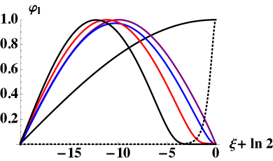
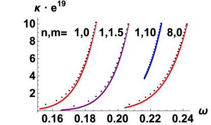
Figure 4: Left: Absolute value of the de Sitter wave functions (40) as a function of $\xi$ for $m=0$, and $l=0,1,2,10,100$ with the maxima normalized to 1. Dashed curve: $\delta V$,  Eq. (50). Right: de Sitter space am-f relations (43) for $\xi_{0}=-20$, (relevant for the inflationary universe) $l\leq 26$ (black dots) in comparison with the Rindler space m-f relations (solid lines) with ${\mathcal{K}}(\omega)$, Eq. (46).

Already for values with angular momenta as small as $l=1$, only a weak overlap between the eigenfunction $\varphi_{1}$ and the difference $\delta V$ is found. On the other hand, due to the absence of the centrifugal barrier the wave-function for $m=0$ and $l=0$ is not dominated by the near horizon region.

These considerations lead us to consider in detail the am-f relation at small angular momenta $l$ where significant differences between de Sitter and Rindler space results occur. On the right hand side of Fig. 4 are shown the discrete eigenvalues for $n=1$ and $m=0,\,1.5,\,10$ (first 3 curves) and $n=8,\,m=0$ together with the corresponding Rindler space m-f relations. The energies $\omega$ of the second and third am-f and m-f relations are shifted by 0.02 and 0.04 respectively and ${\mathcal{K}}(\omega)$ is reduced by a factor of 6 for the $n=8$ am-f and m-f relations. Not included in the figure are the eigenvalues for $l=0$ with exact values $0.0798,\,0.119,\,0.176,\,1.18$ and approximate values $0,\,0.147,\,0.176,0\,$. As suggested by the behavior of the wave functions, the de Sitter am-f relations approach fast the Rindler space m-f relations with increasing $l$ and/or $m$. Already for $l=1,\,m=0$ Rindler and de Sitter space results (cf. Eq. (46)) agree within 4%. The discrepancy can be reduced to 1% by including the next to leading order (cf. Eqs. (44), (45)) in the near horizon approximation. Analytical expression for the l=0 contribution to the partition function For $l=0,\,m=0$ (and $\omega\neq 0$), the near horizon approximation fails. The correspondence (46) assigns to $l=m=0$ the Rindler space value $\tilde{\mathcal{K}}=\omega=0$ (cf. Eq. (17)) independent of the value of $n$ and the next to leading order (44) of the near horizon approximation diverges. However, a closed expression for the am-f relation can be obtained by applying the duplication formula for the $\Gamma$-functions in (42),

$$\omega(\xi_{0}-\ln 2)+(1-\delta_{l=0})\sum_{l^{\prime}=0}^{l-1}\arg(l^{\prime}+i\omega)+\arg(l+1+i\omega)=(-n+1/2)\,\pi\,.$$ (51)

For $l=0$ and not too large values of $n$, the approximate am-f relations are given by,

$$\omega_{n}=-\frac{n-1/2}{\xi_{0}+1-\ln 2}\,\pi\,,$$ (52)

which reproduces the exact values for $n\leq 8$ with an accuracy of 1% or better. On this basis also the $l=0$ contribution to the partition function can be calculated analytically with the result

$$\ln Z_{l=0}=-\sum_{n=1}^{\infty}\ln\bigg{(}1-\exp\Big{(}\frac{(2n-1)\pi^{2}}{\xi_{0}+1-\ln 2}\Big{)}\bigg{)}=1.32\,,$$

which is larger than $\sum_{n}\zeta_{n}$ (first line of Table 1) by a factor of $4.1\cdot 10^{5}$. The relevance of this contribution depends on the density of states which is $1$ for $l=0$ and ${\mathcal{A}}/4\ell^{2}$ (cf. Eq. (11)) for large $l$.

V Angular momentum-energy relations in static spherically symmetric spaces close to horizons

The connection between the am-f and m-f relations of scalar fields in de Sitter and in Rindler space respectively can be generalized to a larger class of static spherically symmetric spaces with a non-extremal horizon. Besides the de Sitter space, the Schwarzschild, the Schwarzschild/AdS or the Reissner-Nordström space belong to this class. The common structure of the line element of this class of spaces reads cf. PADM05 ,

$$ds^{2}=f(r)dt^{2}-\frac{dr^{2}}{f(r)}-r^{2}d\Omega^{2}\,,$$ (53)

with the function $f(r)$ vanishing at $r=r_{0}$ and, close to the horizon, is approximately given by,

$$f(r)\approx(r-r_{0})\,f^{\prime}(r_{0})\,,\quad\text{with}\quad|(r-r_{0})f^{\prime}(r_{0})|=e^{2\kappa\xi}\,,\quad\text{and}\quad 2\kappa=\big{|}f^{\prime}(r_{0})\big{|}\,.$$ (54)

The approximate metric (53) reads,

$$ds^{2}\approx e^{2\kappa\xi}(dt^{2}-d\xi^{2})-r_{0}^{2}\Big{(}1+\frac{1}{2\kappa r_{0}}e^{2\kappa\xi}\Big{)}^{2}d\Omega^{\,2}\approx e^{2\kappa\xi}(dt^{2}-d\xi^{2})-r_{0}^{2}\,d\Omega^{\,2}\,.$$ (55)

The last step of the approximation is valid only if the radial eigenfunctions are concentrated in the region close to the horizon which is never the case for vanishing angular momentum $l$ and mass $m$. The approximate metric (55) is the metric of a product space of the $1+1$ Rindler space and the 2-sphere. Comparison of this metric with the Rindler space metric (2) shows that (up to the normalization) the eigenfunctions are given by the MacDonald functions, which vanish at the boundary (cf. Eq. (9)),

$$K_{i\omega}({\mathcal{K}}_{sp})=0\,,\;\;\;{\mathcal{K}}_{sp}=e^{\xi_{0}}\sqrt{m^{2}+l(l+1)/r^{2}_{0}}\,,$$ (56)

with $\xi_{0},\,r_{0}$ and $m$ given in units of $1/\kappa$ and $\kappa$ respectively. At this point we can proceed as above in identifying the m-f and am-f relations of Rindler and spherical Rindler space respectively.

To test the range of validity of this type of “near horizon approximation”, we apply the above approximation to de Sitter space where, according to Eq. (54),

$$r_{0}=1/\kappa\,,$$ (57)

and the near horizon metric and ${\mathcal{K}}_{sp}$ are given by,

$$ds^{2}=e^{2\xi}(dt^{2}-d\xi^{2})-\,d\Omega^{\,2}\,,\quad{\mathcal{K}}_{sp}=e^{\xi_{0}}\sqrt{m^{2}+l(l+1)}=\left(\frac{m^{2}+l(l+1)}{m^{2}+l(l+3)}\right)^{1/2}{\mathcal{K}}_{dS}\,.$$ (58)

For vanishing $m$ and $l>0$, the two quantities ${\mathcal{K}}_{dS}$ and ${\mathcal{K}}_{sp}$ differ by up to 30% and approach each other with increasing $l$. Trivially at large $l$, but also at small $l$ where the slope of $\omega$ as function of ${\mathcal{K}}$ is of the order of $10^{-3}$, the am-f relations are only weakly affected, i.e., with the exception of the $l=0,m=0$ case, the am-f relations are accurately described by the near horizon approximation (58).

Other examples where this method for calculating the am-f relations and the thermodynamic quantities can be applied to are,

• Schwarzschild metric

  $$f(r)=1-R_{S}/r,\quad\quad R_{S}=2GM,\quad\kappa=1/2R_{S}\,,\quad\kappa r_{0}=\frac{1}{2}\,,$$ (59)

• Schwarzschild/AdS metric

  $$f(r)=1-\frac{R_{S}}{r}+\frac{r^{2}}{R^{2}}\,,\quad\kappa=\frac{1}{R\,b^{2}(\rho)}\big{(}\rho+b^{3}(\rho)\big{)}\,,\quad\kappa r_{0}=\frac{1}{b(\rho)}\big{(}\rho+b^{3}(\rho)\big{)}\,,$$ (60)

  $$\text{with}\quad\rho=\frac{R_{S}}{2R}\,,\quad b(\rho)=\rho^{1/3}\Big{(}\big{(}\sqrt{1+1/27\rho^{2}}+1\big{)}^{1/3}-\big{(}\sqrt{1+1/27\rho^{2}}-1\big{)}^{1/3}\Big{)}\,,$$

• Reissner-Nordström metric

  $$f(r)=1-\frac{R_{S}}{r}+\frac{R^{2}}{r^{2}}\,,\quad R=\ell_{P}\,Q,\quad\text{Planck length}\,\ell_{P},\;\;\text{charge}\,Q,$$ (61)

  $$\rho=\sqrt{1-4R^{2}/R_{S}^{2}}\,,\quad\kappa=\frac{2\rho}{R_{S}(1+\rho)^{2}}\,,\quad\kappa r_{0}=\frac{\rho}{1+\rho}\,.$$

In concluding this section we emphasize the universality of the Rindler space m-f relations (9). Having determined these quantities for a sufficiently large number of modes, as shown in Fig. 1, the (discrete) eigenvalues $\omega(n,l,m,r_{0},\xi_{0})$ for any static spherically symmetric space can be read off from this figure by identifying ${\mathcal{K}}$ with ${\mathcal{K}}_{sp}$ (Eq. (56)) and by taking into account that the scale of any dimensionful quantity is given by the appropriate power of the surface gravity. Evaluation of thermodynamic quantities requires summation over the angular momenta $l$ and the number of zeroes $n$. If the distance to the horizon satisfies $e^{\xi_{0}}\ll 1$ significant contributions to the sum over angular momenta can be expected only if $l\gg 1$ and the summation can be replaced by integration over $l$, cf. Eq. (56), (the summation over $n$ is not replaced by an integration),

$$(2l+1)dl=r_{0}^{2}\,e^{-2\xi_{0}}d({\mathcal{K}}^{2})\,.$$

Therefore the Eqs. (10-13) apply with the area given by,

$$\mathcal{A}=4\pi r_{0}^{2}\,,$$ (62)

while the quantities $\zeta_{n}(\beta,\omega_{n}^{0})$ (Eq. (12)) are “universal”, i.e., independent of the parameters of the static, spherically symmetric metrics with a non-extremal horizon. Qualitatively, this universality was shown in reference PADM86 . Since based on ’t Hooft’s approximation tHOO85 (cf. Eq. (32)) the expressions for the thermodynamic quantities however are incorrect.

VI Conclusions

Momentum- or angular momentum-frequency relations have been shown to be the generic tools for calculating the kinematics of scalar fields in static space-times with a horizon. In particular, in a large range of the kinematics, they exhibit properties which, after choosing appropriate scales, are universal, i.e., independent of the details of the space-times, as our explicit comparison of m-f and am-f relations of Rindler and de Sitter space respectively demonstrates. These relations provide a direct avenue to approximate analytical and accurate numerical computation of the density of states, the essential ingredient for the thermodynamics of fields in spaces with a horizon. The central results for the thermodynamic quantities is summarized in expression (26) and Table 1 which imply that up to a correction of less than 1%, partition function and entropy are generated by a single mode, i.e., black holes are low temperature systems. This property applies not only for the scalar fields in Rindler spaces but also, as we have seen explicitly, for fields in de Sitter space and more generally in static, spherically symmetric spaces. Our results are in conflict with most of the results obtained by applying the brick wall method. In order to arrive at closed expressions it has become common to replace the discrete spectrum of eigenmodes by a continuous one. We have shown in detail that this procedure cannot be justified and gives rise to values of the thermodynamic quantities which are too large by two orders of magnitude.

New insights into the dynamics of quantum fields of higher spin, in particular of photons, cf. KABT95 , COLE98 , DOWA12 and gravitons via m-f or am-f relations can be expected. The imaginary parts of the corresponding stationary propagators LOY11 , closely related to the m-f relations, indicate significant differences between fields of different spin. Also the application to fields in rotating black holes HKPS97 , MUKO00 , CHLY09 promises to introduce a new element in the role of the probably complex m-f and am-f relations. With the one mode dominance of the thermodynamic quantities, a hidden “parameter” specifying the boundary condition, emerges which, as we have seen, (cf. Eq. (37)), influences severely partition function and entropy and needs to be determined.

*

Appendix A Failure of the Modified WKB approximation

In order to identify in detail the large effect of replacing the $n$-sum with $n\geq 1$ by an integral with $0$ as lower limit we introduce the following two functions $\sigma(\omega,\nu_{0})$ and $\rho(\nu)$, cf. Eq. (32),

$$\sigma(\omega,\nu_{0})=\frac{\beta}{\pi}\,\hat{\mathcal{K}}^{2}_{1}(\omega)\int_{\nu_{0}}^{\infty}d\nu\frac{\nu^{3}}{e^{\beta\nu\omega}-1}\,,\hskip 18.49411pt\rho(\nu)=\frac{\beta}{\pi}\,\nu^{3}\int_{0}^{\infty}d\omega\frac{1}{e^{\beta\nu\omega}-1}\hat{\mathcal{K}}^{2}_{1}(\omega)\,,$$ (63)

which, if integrated,

$$\ln\hat{Z}_{apx}=\frac{{\mathcal{A}}}{4\ell^{2}}\,\int_{0}^{\infty}d\omega\,\sigma(\omega,\nu_{0})=\frac{{\mathcal{A}}}{4\ell^{2}}\,\int_{\nu_{0}}^{\infty}d\nu\,\rho(\nu)\,,$$

yield the approximate value of the partition function (34) provided $\nu_{0}=0$.

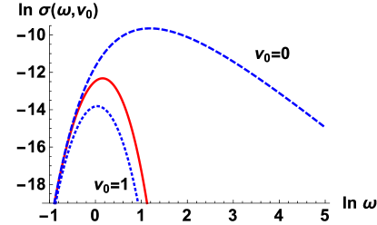
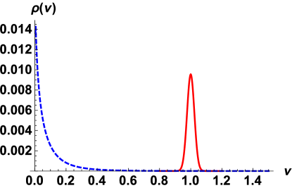
Figure 5: Left: Solid (red) line: Density $\hat{\sigma}(\omega)$ cf. Eq. (28). Dashed and dotted (blue) lines: $\sigma(\omega,\nu_{0})$, Eq. (63), with $\nu_{0}=0$ and $\nu_{0}=1$ respectively Right: Dotted (blue) line: density $\rho(\nu)$ (Eq.(63)), solid (red) line: the $n=1$ contribution multiplied by a factor 235 with a Gaussian distribution replacing $\delta(\nu-1)$ (cf. text).

The left hand side of Fig. 5 demonstrates the high sensitivity of the partition function $\hat{Z}_{apx}$ when varying the lower limit of the $\omega$ integration. Replacing the lower limit $\nu_{0}=0$ of the “standard” approximation (32) by $\nu_{0}=1$ reduces the value of the maximum of $\sigma(\omega,\nu)$ by a factor of 67 and the corresponding half width by a factor of 5. As the right hand side of Fig. 5 shows, the dominant contribution to the partition function actually arises from values of $\nu$ in the interval $0<\nu\leq 0.4$ and the integration over the interval $0\leq\nu\leq 1$ reproduces the analytically determined value of the partition function (34) up to 0.1%.

In summary, it is not a large number of modes which contribute and give rise to a large value of the partition function which would justify the approximation (32). Rather it is the contributions from the unphysical region, $\nu<1$, which generate the large value of $\ln\hat{Z}_{apx}$ (Eq. (34)) exceeding the correct value by a factor of 235.

References

- (1) G. ’t Hooft, Nucl. Phys. B256, (1985), 727, “On the quantum structure of a black hole”
- (2) L. Susskind and J. Uglum, Phys. Rev. D 50, (1994), 2700, “Black hole entropy in canonical quantum gravity and superstring theory”
- (3) G. ’t Hooft, Int. J. Mod.Phys. A11, (1996), 4623, “The scattering matrix approach for the quantum black hole, an overview”
- (4) S. Mukohyama and W. Israel, Phys. Rev. D 58, (1998), 104005-1, “Black Holes, brick walls, and the Boulware state”
- (5) V. Frolov and D. V. Fursaev, Class. Quantum Grav. 15, (1998), 2041, “Thermal fields, entropy and black holes”
- (6) T. Padmanabhan, Phys. Rep. 406, (2005), 49, “Gravity and the thermodynamics of horizons”
- (7) S. Sarkar, S. Shankaranarayanan and L. Siramkumar, Phys. Rev. D 78, (2008), 024003, “Subleading contributions to the black hole entropy in the brick wall approach”
- (8) W. Kim and S. Kulkarni, Eur. Phys. J. C 73:2398 (2013), “Higher order WKB corrections to black hole entropy in brick wall formalism”
- (9) J. Demers, R. Lafrance and C. Myers Phys. Rev. D 52, (1995), 2245, “Black hole entropy without brick walls”
- (10) T. Padmanabhan, Phys. Lett. B 173, (1986), 43, “On the quantum structure of horizons”
- (11) W. Rindler, “Relativity, Special, General and Cosmological”, Oxford University Press 2001
- (12) R. M. Wald, “Quantum Field Theory in Curved Spacetime and Black Hole Thermodynamics”, The University of Chicago Press 1994
- (13) F. Lenz, K. Ohta and K. Yazaki, Phys. Rev. D 78, (2008), 065026, “Canonical quantization of gauge fields in static space-times with applications to Rindler space”
- (14) W. G. Unruh, Phys. Rev. D 14, (1976), 870, “Notes on black hole evaporation”
- (15) I. S. Gradshteyn and I. M. Ryzhik, Table of Integrals, Series and Products, Academic Press 1965
- (16) F. Lenz, K. Ohta and K. Yazaki, Phys. Rev. D 83, (2011), 064037, “Static interactions and stability of matter in Rindler space”
- (17) D. Kabat and M. Strassler, Phys. Lett. B 329, (1994), 46, “A comment on entropy and area”
- (18) M. Spradlin, A. Strominger and A. Volovich, [arXiv:hep-th/010007], “Les Houches Lectures on de Sitter space”
- (19) D. Lohiya and N. Panchapakesan, J. Phys. A 11, (1978), 1963, “Massless scalar fields in a de Sitter universe and its thermal flux”
- (20) M. M. Abramowitz and A. Stegun, Handbook of Mathematical Functions, Dover Publications, New York 1965,
- (21) D. Kabat, Nucl. Phys. B453, (1995), 281, “Black hole entropy and entropy of entanglement”
- (22) G. Cognola and P. Lecca, Phys. Rev. D 57, (1998), 1108, “Electromagnetic fields in Schwarzschild and Reissner-Nordström geometry: Quantum corrections to the black hole entropy”
- (23) W. Donnelly and A. Wall, Phys. Rev. D86, (2012), 064042, “Do gauge fields really contribute negatively to black hole entropy”
- (24) J. Ho, W. Kim, Y. Park and H. Shin, Class. Quantum Grav. 14, (1997), 2617, “Entropy in the Kerr-Newman black hole”
- (25) S. Mukohyama, Phys. Rev. D 61, (2000), 124021, “Is the brick-wall model stable for a rotating background”
- (26) E. Chang-Young, D. Lee and M. Yoon, Class. Quantum Grav. 26, (2009), 155011, “Rotating black hole entropy from two different viewpoints”