Discovering the Network Backbone from Traffic Activity Data

Abstract

We introduce a new computational problem, the BackboneDiscovery problem, which encapsulates both functional and structural aspects of network analysis. While the topology of a typical road network has been available for a long time (e.g., through maps), it is only recently that fine-granularity functional (activity and usage) information about the network (like source-destination traffic information) is being collected and is readily available. The combination of functional and structural information provides an efficient way to explore and understand usage patterns of networks and aid in design and decision making. We propose efficient algorithms for the BackboneDiscovery problem including a novel use of edge centrality. We observe that for many real world networks, our algorithm produces a backbone with a small subset of the edges that support a large percentage of the network activity.

1 Introduction

In this paper we study a novel problem, which combines structural and functional (activity) network data. In recent years there has been a large body of research related to exploiting structural information of networks. However, with the increasing availability of fine-grained functional information, it is now possible to obtain a detailed understanding of activities on a network. Such activities include source-destination traffic information in road and communication networks.

More specifically we study the problem of discovering the backbone of traffic networks. In our setting, we consider the topology of a network ${G}=({V},{E})$ and a traffic log ${\cal L}=\{({s}_{i},{t}_{i},{w}_{i})\}$, recording the amount of traffic ${w}_{i}$ that incurs between source ${s}_{i}$ and destination ${t}_{i}$. We are also given a budget $B$ that accounts for a total edge cost. The goal is to discover a sparse subnetwork $R$ of $G$, of cost at most $B$, which summarizes as well as possible the recorded traffic $\cal L$.

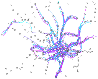
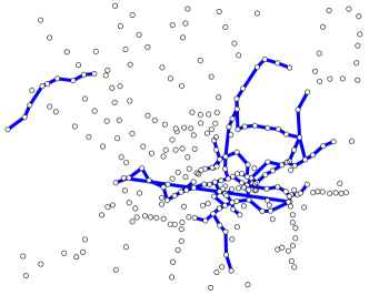
Figure 1: London tube network, with nodes representing the stations. The figure on the left shows a subset of the trips made, and the figure on the right shows the corresponding backbone, as discovered by our algorithm. The input data contains only source–destination (indicating start and end points of a trip) pairs and for visualization purposes, a B-spline was interpolated along the shortest path between each such pair. The backbone presented on the right covers only 24% of the edges in the original network and has a stretch factor of 1.58. This means that even with pruning 76% of the edges in the network, we are able to maintain shortest paths which are at most 1.58 times the shortest path length original graph.

The problem we study has applications for both exploratory data analysis and network design. An example application of our algorithm is shown in Figure 1. Here, we consider a traffic log (Figure 1, left), which consists of the most popular routes used on the London tube. The backbone produced by our algorithm takes into account this demand (based on the traffic log) and tries to summarize the underlying network, thus presenting us with insights about usage pattern of the London tube (Figure 1, right). This representation of the ‘backbone’ of the network could be very useful to identify the important edges to upgrade or to keep better maintained in order to minimize the total traffic disruptions.

We only consider source-destination pairs in the traffic log, and not full trajectories, as source-destination information captures true mobility demand in a network. For example, data about the daily commute from home (source) to office (destination) is more resilient than trajectory information, which is often determined by local and transient constraints, like traffic conditions on the road, time of day, etc. Furthermore, in communication networks, only the source-ip and destination-ip information is encoded in TCP-IP packets. Similarly, in a city metro, check-in and check-out information is captured while the intervening movement is not logged.

The BackboneDiscovery problem is an amalgam of the $k$-spanner problem [15] and the Steiner-forest problem [23]. However, our problem formulation will have elements which are substantially distinct from both of these problems.

In the $k$-spanner problem the goal is to find a minimum-cost subnetwork $R$ of $G$, such that for each pair of nodes $u$ and $v$, the shortest path between $u$ and $v$ on $R$ is at most $k$ times longer than the shortest path between $u$ and $v$ on $G$. In our problem, we are not necessarily interested in preserving the $k$-factor distance between all nodes but for only a subset of them.

In the Steiner-forest problem we are given a set of pairs of terminals $\{({s}_{i},{t}_{i})\}$ and the goal is to find a minimum-cost forest on which each source ${s}_{i}$ is connected to the corresponding destination ${t}_{i}$. Our problem is different from the Steiner-forest problem because we do not need all $\{({s}_{i},{t}_{i})\}$ to be connected, and try to optimize a stretch factor so that the structural aspect of the network are also taken into account.

A novel aspect of our work is the use of edge-betweenness to guide the selection of the backbone [17]. The intuition is as follows. An algorithm to solve the Steiner-forest problem will try and minimize the sum of cost of edges selected as long as as the set of terminal pairs $\{({s}_{i},{t}_{i})\}$ are connected and is agnostic to minimizing stretch factor. However, if the edge costs are inversely weighted with edge-betweenness, then edges that can contribute to reducing the stretch factor can be potentially included into the backbone.

To understand the differences of the proposed BackboneDiscovery problem with both the $k$-spanner and Steiner-forest formulations, consider the example shown in Figure 2. In this example, there are four groups of nodes:

1. group $A$ consists of $n$ nodes, $a_{1},\ldots,a_{n}$,

2. group $B$ consists of $n$ nodes, $b_{1},\ldots,b_{n}$,

3. group $C$ consists of $2$ nodes, $c_{1}$ and $c_{2}$, and

4. group $D$ consists of $m$ nodes, $d_{1},\ldots,d_{m}$.

Assume that $m$ is smaller then $n$, and thus much smaller than $n^{2}$. All edges shown in the figure have cost $1$, except the edges between $c_{1}$ and $c_{2}$, which has cost $2$. Further assume that there is one unit of traffic between each $a_{i}$ and each $b_{j}$, for $i,j=1,\ldots,n$, resulting in $n^{2}$ source-destination pairs (the majority of the traffic), and one unit of traffic between $d_{i}$ and $d_{i+1}$, for $i=1,\ldots,m-1$, resulting in $m-1$ source-destination pairs (some additional marginal traffic). The example abstracts a common layout found in many cities: a few busy centers (commercial, residential, entertainment, etc.) with some heavily-used links connecting them (group $C$), and some peripheral ways around, that serve additional traffic (group $D$).

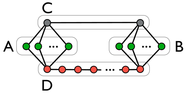
(a)

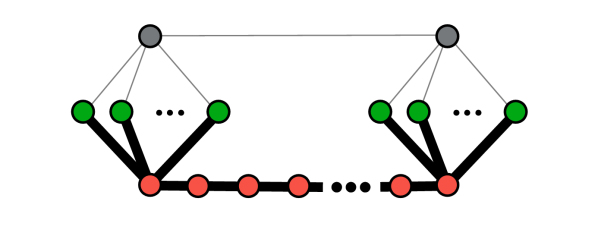
(b)

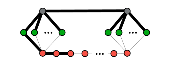
(c)

Figure 2: The BackboneDiscovery problem solution results in a better network than the one obtained from the Steiner forest solution. (a) A traffic network. We consider a unit of traffic from each node in $A$ to each node in $B$, and from each node in $D$ to its right neighbor. (b) Shown with thick edges is an optimal Steiner forest for certain cost $C$. (c) Shown with thick edges is a backbone of cost at most $C$ that captures the traffic in the network better than the optimal Steiner forest.

Careful inspection of the above example highlights advantages of the backbone discovery problem:

• As opposed to the $k$-spanner problem, we do not need to guarantee short paths for all pairs of nodes, but only for those in our traffic log which makes our approach more general. In particular, based on the budget requirements a backbone could be designed for the most voluminous paths.

• Due to the budget constraint, it may not be possible to guarantee connectivity for all pairs in the traffic log. We thus need a way to decide which pairs to leave disconnected. Neither the $k$-spanner nor the Steiner-forest problems provision for disconnected pairs. In fact, it is possible that the optimal backbone may even contain cycles while leaving pairs disconnected. Again, allowing for a disconnected backbone, generalizes the Steiner-forest problem and may help provision for a tighter budget. In order to allow for a disconnected backbone, we employ the use of stretch factor, defined as a weighted harmonic mean over the source-destination pairs of the traffic log, which provides a principled objective to optimize connectivity while allowing to leave disconnected pairs, when there is insufficient budget.

• Certain high cost edges may be an essential part of the backbone that other problem formulations may leave out. For example, while the edge that connects the nodes in $C$ is a very important edge for the overall traffic (as it provides a short route between $A$ and $B$), the optimal Steiner-forest solution, shown in Figure 2b, prefers the long path along the nodes in $D$. Our algorithm includes the component $C$ (as seen in Figure 2c) because it is an edge that has a high edge-betweenness.

The rest of the paper is organized as follows. In Section 2, we rigorously define the BackboneDiscovery problem. Section 3 introduces our algorithm based on the greedy approach, Section 4 details our experimental evaluation, results and discussion. In Section 5 we survey related work and distinguish our problem formulation with other relevant approaches. We conclude in Section 6 with a summary and potential directions for future work.

2 Problem definition

Let ${G}=({V},{E})$ be a network, with $|{V}|={n}$ and $|{E}|={m}$. For each edge ${e}\in{E}$ there is a cost ${c}({e})$. Additionally, we consider a traffic log $\cal L$, specified as a set of triples $({s}_{i},{t}_{i},{w}_{i})$, with ${s}_{i},{t}_{i}\in{V}$, and with $i=1,\ldots,{k}$. A triple $({s}_{i},{t}_{i},{w}_{i})$ indicates the fact that ${w}_{i}$ units of traffic have been recorded between nodes ${s}_{i}$ and ${t}_{i}$.

We aim at discovering the backbone of traffic networks. A backbone ${R}$ is a subset of the edges of the network ${G}$, that is, ${R}\subseteq{E}$ that provides a good summarization for the whole traffic in $\cal L$. In particular, we require that if the available traffic had used only edges in the backbone $R$, it should have been almost as efficient as using all the edges in the network. We formalize this intuition below.

Given two nodes ${s},{t}\in{V}$ and a subset of edges ${A}\subseteq{E}$, we consider the shortest path ${d}_{A}({s},{t})$ from $s$ to $t$ that uses only edges in the set $A$. In this shortest-path definition, edges are counted according to their cost $c$. If there is no path from ${s}$ to ${t}$ using only edges in $A$, we define ${d}_{A}({s},{t})=\infty$. Consequently, ${d}_{E}({s},{t})$ is the shortest path from ${s}$ to ${t}$ using all the edges in the network, and ${d}_{R}({s},{t})$ is the shortest path from ${s}$ to ${t}$ using only edges in the backbone $R$.

To measure the quality of a backbone $R$, with respect to some traffic log ${\cal L}=\{({s}_{i},{t}_{i},{w}_{i})\}$ we use the concept of stretch factor. Intuitively, we want to consider shortest paths from ${s}_{i}$ to ${t}_{i}$, and evaluate how much longer are those paths on the backbone $R$, than on the original network. The idea of using stretch factor for evaluating the quality of a subgraph has been used extensively in the past in the context of spanner graphs [15].

In order to aggregate shortest-path information for all source–destination pairs in our log in a meaningful way, we need to address two issues. The first issue is that not all source–destination pairs have the same volume in the traffic log. This can be easily addressed by weighting the contribution of each pair $({s}_{i},{t}_{i})$ by its corresponding volume ${w}_{i}$.

The second issue is that since we aim at discovering very sparse backbones, many source–destination pairs in the log could be disconnected in the backbone. To address this problem we aggregate shortest-path distances using the harmonic mean. This idea, which has been proposed by Marchiori and Latora [12] and has also been used by Boldi and Vigna [1] in measuring centrality in networks, provides a very clean way to deal with infinite distances: if a source–destination pair is not connected, their distance is infinity, so the harmonic mean accounts for this by just adding a zero term in the summation. Using the arithmetic mean is problematic, as we would need to add an infinite term with other finite numbers.

Overall, given a set of edges ${A}\subseteq{E}$, we measure the connectivity of the traffic log ${\cal L}=\{({s}_{i},{t}_{i},{w}_{i})\}$, $|{\cal L}|=k$ by

$${H}_{\cal L}({A})=\left(\sum_{i=1}^{k}{w}_{i}\right)\left(\sum_{i=1}^{k}\frac{{w}_{i}}{{d}_{A}({s}_{i},{t}_{i})}\right)^{-1}.$$

The stretch factor of a backbone $R$ is then defined as

$${\lambda}_{\cal L}({R})=\frac{{H}_{\cal L}({R})}{{H}_{\cal L}({E})}.$$

The stretch factor is always greater or equal than 1. The closer it is to 1, the better the connectivity that it offers to the traffic log $\cal L$.

We are now ready to formally define the problem of backbone discovery.

Problem 1 (BackboneDiscovery)

Consider a network ${G}=({V},{E})$ and a traffic log ${\cal L}=\{({s}_{i},{t}_{i},{w}_{i})\}$. Consider also a cost budget $B$. The goal is to find a backbone network ${R}\subseteq{E}$ of total cost $B$ that minimizes the stretch factor ${\lambda}_{\cal L}({R})$ or report that no such solution exists.

As one may suspect, BackboneDiscovery is an $\mathbf{NP}$-hard problem.

Lemma 1

The BackboneDiscovery problem, defined in Problem 1, is $\mathbf{NP}$-hard.

Proof 2.1 (Sketch).

We obtain a reduction from the SetCover problem: given a ground set ${U}=\{{u}_{1},\ldots,{u}_{n}\}$, a collection ${\cal S}=\{{S}_{1},\ldots,{S}_{m}\}$ of subsets of $U$, and an integer $k$, determine whether there are $k$ sets in $\cal S$ that cover all the elements of $U$.

Given an instance of the SetCover problem we form an instance of the BackboneDiscovery problem as follows (See Figure 3 for illustration). We create one node ${u}_{i}$ for each ${u}_{i}\in{U}$ and one node ${v}_{j}$ for each ${S}_{j}\in{\cal S}$. We also create a special node ${z}$. We create an edge $({u}_{i},{v}_{j})$ if and only if ${u}_{i}\in{S}_{j}$ and we assign to this edge cost 0. We also create an edge $({v}_{j},{z})$ for all ${S}_{j}\in{\cal S}$ and we assign to this edge cost 1. As far as the traffic log is concerned, we set ${\cal L}=\{({u}_{i},{z},1)\mid{u}_{i}\in{U}\}$, that is, we pair each ${u}_{i}\in{U}$ with the special node $z$ with volume 1. Finally we set the budget ${B}={k}$. It is not difficult to see that the instance of the BackboneDiscovery problem constructed in this way has a solution with stretch factor 1 if and only if the given instance of the SetCover problem has a feasible solution.

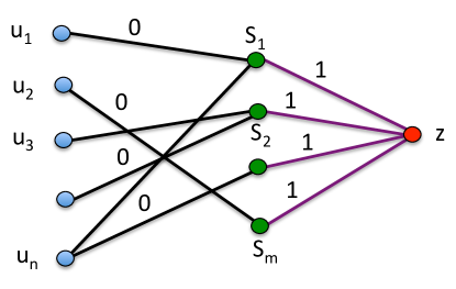
Figure 3: Reduction from Set Cover to BackboneDiscovery for the log ${\cal L}=\{(u_{i},z,1)|u_{i}\in U\}$

3 Algorithm

The algorithm we propose for the BackboneDiscovery problem is a greedy heuristic that connects one-by-one the source–destination pairs of the traffic log $\cal L$. A distinguishing feature of our algorithm is that it utilizes a notion of edge benefit. In particular, we assume that for each edge ${e}\in{E}$ we have available a benefit measure ${b}({e})$. The higher is the measure ${b}({e})$ the more beneficial it is to include the edge $e$ in the final solution. The benefit measure is computed using the traffic log $\cal L$ and it takes into account the global structure of the network $G$.

The more central an edge is with respect to a traffic log, the more beneficial it is to include it in the solution, as it can be used to serve many source–destination pairs. In this paper we use edge-betweenness as a centrality measure, adapted to take into account the traffic log. We also experimented with commute-time centrality, but edge-betweenness was found to be more effective.

Our algorithm relies on the notion of effective distance ${\widehat{\ell}}({e})$, defined as ${\widehat{\ell}}({e})={c}({e})/{b}({e})$, where ${c}({e})$ is the cost of an edge ${e}\in{E}$, and ${b}({e})$ is the edge-betweenness of $e$. The intuition is that by dividing the cost of each edge by its benefit, we are biasing the algorithm towards selecting edges with high benefit.

We now present our algorithm in more detail.

3.1 The greedy algorithm.

As discussed above, our algorithm operates with effective distances ${\widehat{\ell}}({e})={c}({e})/{b}({e})$, where ${b}({e})$ is a benefit score for each edge $e$. The objective is to obtain a cost/benefit trade-off: edges with small cost and large benefit are favored to be included in the backbone. In the description of the greedy algorithm that follows, we assume that the effective distance ${\widehat{\ell}}({e})$ of each edge is given as input.

The algorithm works in an iterative fashion, maintaining and growing the backbone, starting from the empty set. In the $i$-th iteration the algorithm picks a source–destination pair $({s}_{i},{t}_{i})$ from the traffic log $\cal L$, and “serves” it. Serving a pair $({s}_{i},{t}_{i})$ means computing a shortest path ${p}_{i}$ from ${s}_{i}$ to ${t}_{i}$, and adding its edges in the current $R$, if they are not already there. For the shortest-path computation the algorithm uses the effective distances ${\widehat{\ell}}({e})$. When an edge is newly added to the backbone its cost is subtracted from the available budget. Here, the actual cost of the edge ${c}({e})$ (instead of the ${\widehat{\ell}}({e})$) is used. Also its effective distance is reset to zero, since it can be used for free in subsequent iterations of the algorithm. The source–destination pair that is chosen to be served in each iteration is the one that reduces the stretch factor the most at that iteration; and hence the greedy nature of the algorithm.

The algorithm proceeds until it exhausts all its budget or until the stretch factor becomes equal to 1 (which means that all pairs in the log are served via a shortest path). The pseudo-code for the greedy algorithm is shown as Algorithm 1.

Algorithm 1 The greedy algorithm

0:  Network ${G}=({V},{E})$, edge costs ${c}({e})$, benefit costs ${b}({e})$, cost budget $B$, traffic log ${\cal L}=\{({s}_{i},{t}_{i},{w}_{i})\}$

0:   A subset of edges ${R}\subseteq{E}$ of total cost ${c}({R})\leq{B}$ and small stretch factor ${\lambda}({R})$

1:  for all ${e}\in{E}$ do

2:     ${\widehat{\ell}}({e})\leftarrow{c}({e})/{b}({e})$

3:  ${R}\leftarrow\emptyset$

4:  ${\lambda}\leftarrow\infty$

5:  while $({B}>0)$ and $({\lambda}>1)$ do

6:     for  each $({s}_{i},{t}_{i},{w}_{i})\in{\cal L}$  do

7:        ${p}_{i}\leftarrow$ShortestPath$({s}_{i},{t}_{i},{G},{\widehat{\ell}})$

8:        ${\lambda}_{i}\leftarrow$StretchFactor$({R}\cup{p}_{i},{G},{\cal L})$

9:     $p^{*}\leftarrow\min_{i}\{{\lambda}_{i}\}$ // the path with min. stretch factor in the above iteration

10:     ${R}^{\prime}\leftarrow p^{*}\setminus{R}$ // edges to be newly added

11:     if ${c}({R}^{\prime})>{B}$ then

12:        Return ${R}$ // budget exhausted

13:     ${R}\leftarrow{R}\cup{R}^{\prime}$ // add new edges in the backbone

14:     ${\widehat{\ell}}({R}^{\prime})\leftarrow 0$ // reset cost of newly added edges

15:     ${B}\leftarrow{B}-{c}({R}^{\prime})$ // decrease budget

16:     ${\lambda}\leftarrow$StretchFactor$({R},{G},{\cal L})$ // update ${\lambda}$

17:  Return ${R}$

We are experimenting with two variants of this greedy scheme, depending on the benefit score we use. These are the following:

Greedy:

We use uniform benefit scores (${b}({e})=1$).

GreedyEB:

The benefit score of an edge is set equal to its edge-betweenness centrality.

3.2 Speeding up the greedy algorithm.

As we show in the experimental section the greedy algorithm provides solutions of good quality, in particularly the variant with the edge-betweenness weighting scheme. However, the algorithm is computationally expensive, and thus in this section we discuss a number of optimizations. We start by analyzing the running time of the algorithm.

Running time. Assume that the benefit scores ${b}({e})$ are given for all edges ${e}\in{E}$, and that the algorithm performs $I$ iterations until it exhausts its budget. In each iteration we need to perform ${\cal O}({k}^{2})$ shortest-path computations, where $k$ is the size of the traffic log $\cal L$. A shortest path computation is ${\cal O}({m}+{n}\log{n})$, and thus the overall complexity of the algorithm is ${\cal O}({I}{k}^{2}({m}+{n}\log{n}))$. The number of iterations $I$ depends on the available budget and in the worst case it can be as large as $k$. However, since we aim at finding sparse backbones, the number of iterations is typically smaller.

Optimizations with no approximation. We first show how to speed up the algorithm, while guaranteeing the same solution with the naïve implementation of the greedy. Since the most expensive component is the computation of shortest paths on the newly-formed network, we make sure that we compute the shortest path only when needed. Our optimizations consist of two parts.

First, during the execution of the algorithm we maintain the connected components that the backbone creates in the network. Then, we do not need to compute shortest paths for all $({s}_{i},{t}_{i})$ pairs, for which ${s}_{i}$ and ${t}_{i}$ belong to different connected components; we know that their distance is $\infty$. This optimization is effective at the early stages of the algorithm, when many terminals belong to different connected components.

Second, when computing the decrease in the stretch factor due to a candidate shortest path to be added in the backbone, for pairs for which we have to recompute a shortest-path distance, we first compute an optimistic lower bound, based on the shortest path on the whole network (which we compute once in a preprocessing step). If this optimistic lower bound is not better than the current best stretch factor then we can skip the computation of the shortest path on the backbone.

As shown in the empirical evaluation of our algorithms, depending on the dataset, these optimization heuristics lead to 20–35% improvement in performance.

Optimization based on landmarks. To further improve the running-time of the algorithm we compute shortest-path distances using landmarks [6, 18], an effective technique to approximate distances on graphs. Here we use the approach of Potamias et al. [18]: A set of $\ell$ landmarks ${L}=\{{z}_{1},\ldots,{z}_{\ell}\}$ is selected and for each vertex ${v}\in{V}$ the distances ${d}({v},{z}_{i})$ to all landmarks are computed and stored as an ${\ell}$-dimensional vector representing vertex $v$. The distance between two vertices ${v}_{1},{v}_{2}$ is then approximated as $\min_{i}\{{d}({v}_{1},{z}_{i})+{d}({v}_{2},{z}_{i})\}$, i.e., the tightest of the upper bounds induced by the set of landmarks $L$.

To select landmarks we use high-degree non-adjacent vertices in the graph, which is reported as one of the best performing methods by Potamias et al. [18]. Note that the distances are now approximations to the true distances, and the method trades accuracy by efficiency via the number of landmarks selected. In practice a few hundreds of landmarks are sufficient to provide high-quality approximations even for graphs with millions of vertices [18].

For the running-time analysis, note that in each iteration we need to compute the distance between all graph vertices and all landmarks. This can be done with $\ell$ single-source shortest-path computations and the running time is ${\cal O}({\ell}({m}+{n}\log{n}))$. The landmarks can then be used to approximate shortest-path distances between all source-destination pairs in the traffic log $\cal L$, with running time ${\cal O}({k}{\ell})$. Thus, the overall complexity is ${\cal O}({I}{\ell}({k}+{m}+{n}\log{n}))$. Since $\ell$ is expected to be much smaller than $k$, the method provides a significant improvement over the naïve implementation of the greedy. As shown in the experimental evaluation, using landmarks provides an improvement of up to 4 times in terms of runtime in practice.

3.3 Edge-betweenness centrality.

As we already discussed in the previous sections, our greedy algorithm uses edge centrality measures for benefit scores ${b}({e})$. In this section we discuss edge betweenness, and in particular show how we adapt the measure to take into account the traffic log $\cal L$.

We first recall the standard definition of edge-betweennes. Given a network ${G}=({V},{E})$, we define ${{V}_{2}}={{V}\choose 2}$ to be the set of all pairs of nodes of ${G}$. Given a pair of nodes $({s},{t})\in{{V}_{2}}$ and an edge ${e}\in{E}$, we define by ${\sigma}_{{s},{t}}$ the total number of shortest paths from ${s}$ to ${t}$, and by ${\sigma}_{{s},{t}}({e})$ the total number of shortest paths from ${s}$ to ${t}$ that pass though edge $e$.

The standard definition of edge-betweenness centrality ${EB}({e})$ of edge $e$ is the following:

$${EB}({e})=\sum_{({s},{t})\in{{V}_{2}}}\frac{{\sigma}_{{s},{t}}({e})}{{\sigma}_{{s},{t}}}.$$

In our problem setting we take into account the traffic log ${\cal L}=\{({s}_{i},{t}_{i},{w}_{i})\}$, and we define the edge-betweenness ${EB_{{\cal L}}}({e})$ of an edge $e$ with respect to log $\cal L$, as follows.

$${EB_{{\cal L}}}({e})=\sum_{({s},{t},{w})\in{\cal L}}{w}\,\frac{{\sigma}_{{s},{t}}({e})}{{\sigma}_{{s},{t}}}.$$

In this modified definition only the source–destination pairs of the log $\cal L$ contribute to the centrality of the edge $e$, and the amount of contribution is proportional to the corresponding traffic. The adapted edge-betweenness can still be computed in ${\cal O}({n}{m})$ time [3].

4 Experimental evaluation

The aim of the experimental section is to evaluate the performance of the proposed algorithm, the optimizations, and the edge-betweenness measure. We also compare our algorithm with other state-of-the-art methods which attempt to solve a similar problem.

Datasets. We experiment with six real-world datasets, four transportation networks, one web network and one internet-traffic network. For five of the datasets we also obtain real-world traffic, while for one we use synthetically-generated traffic. The characteristics of our datasets are provided in Table 1, and a brief description follows.

Dataset	Type	# Nodes	# Edges	Real	Real
				network	traffic
LondonTube	transportation	316	724	✓	✓
USFlights	transportation	1 268	51 098	✓	✓
UKRoad	transportation	8 341	13 926	✓	-
NYCTaxi	transportation	50 736	158 898	✓	✓
Wikispeedia	web	4 604	213 294	✓	✓
Abeline	internet	12	15	✓	✓

Table 1: Dataset statistics.

LondonTube. The London Subway network consists of subway stops and links between them. We use the geographic distance between stations as a proxy for edge costs. We also obtain a traffic log ${\cal L}$ extracted from the Oyster card system. The log consists of aggregate trips made by passengers between pairs of stations during a one-month period (Nov-Dec 2009). We filter out source-destination pairs with traffic less than 100 and remove bi-directional pairs by selecting one of them at random and summing up their traffic.

USFlights. We obtain a large network of US airports, and the list of all flights within the US during 2009–2013, from the Bureau of Transportation Statistics. Flying distances between airports, obtained using Travelmath.com, are used as edge costs. The traffic volume is the number of flights between airports.

NYCTaxi. We obtain the complete road network of NYC using OpenStreetMap data. In this network each node corresponds to a road intersection and each link corresponds to a road segment. Edge costs are computed as the geographic distances between the junctions. Data on the pickup and drop-off locations of NYC taxis for 2013 was used to construct the traffic log. The $2\,000$ most frequently used source-destination pairs was used to create the traffic log.

Wikispeedia. Wikispeedia [22] is an online crowd sourcing game designed to measure semantic distances between 2 wikipedia pages using the paths taken by humans to reach from one page to the other. This dataset contains a base network of hyperlinks between Wikipedia pages and the paths taken by users between two pages. We construct the traffic log using the unique (start, end) pages from this data.

UKRoad. Next we consider the UK road network. The network construction is similar to what was done with the NYCTaxi data. For simplicity we use only the largest connected component. Since we were not able to obtain real-world traffic data for this network, we generate synthetic traffic logs ${\cal L}$ simulating different scenarios. In particular we generate traffic logs according to four different distributions: ($i$) power-law traffic volume, power-law $s$-$t$ pairs; ($ii$) power-law traffic volume, uniformly random $s$-$t$ pairs; ($iii$) uniformly random traffic volume, power-law $s$-$t$ pairs; and ($iv$) uniformly random traffic volume, uniformly random $s$-$t$ pairs. These different distributions capture different traffic volume possibility and hence help in understanding the behavior of our algorithm with respect to the traffic log ${\cal L}$.

Abeline. For a qualitative analysis we also consider the well known Abeline dataset consisting of a sample of the network traffic extracted from the Internet2 backbone and that carries the network traffic between major universities in the continental US. The network consists of twelve nodes and 15 high-capacity links. Associated with each physical link, we also have capacity of the link which serves as a proxy for the cost of the link. We obtain traffic logs from 2003 between all pairs of nodes.

Baseline. To obtain better intuition for the performance of our methods we define a simple baseline, where a backbone is created by adding edges in increasing order of their effective distances ${\widehat{\ell}}({e})={c}({e})/{b}({e})$, where ${b}({e})$ is edge-betweenness; this was the best-performing baseline among other baselines we tried, such as adding source–destination pairs one by one (i) randomly, (ii) in decreasing order of volume ($w_{i}$), (iii) in increasing order of effective distance defined using closeness centrality, etc.

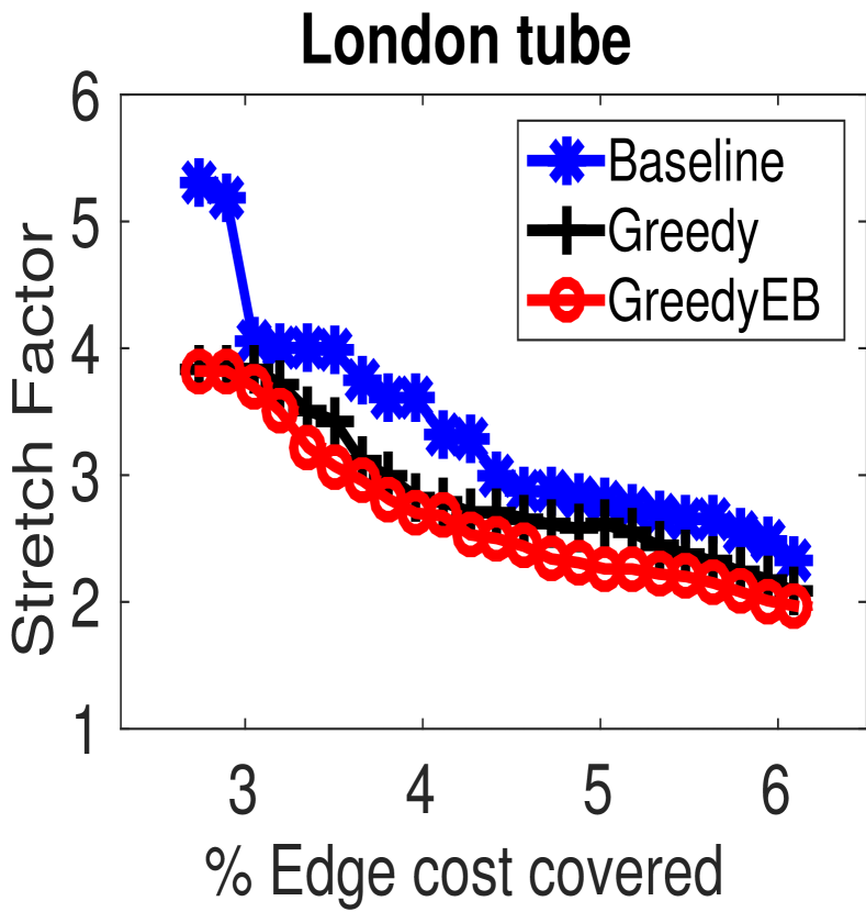
(a)

(b)

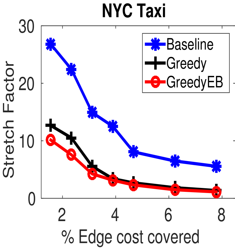
(c)

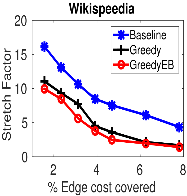
(d)

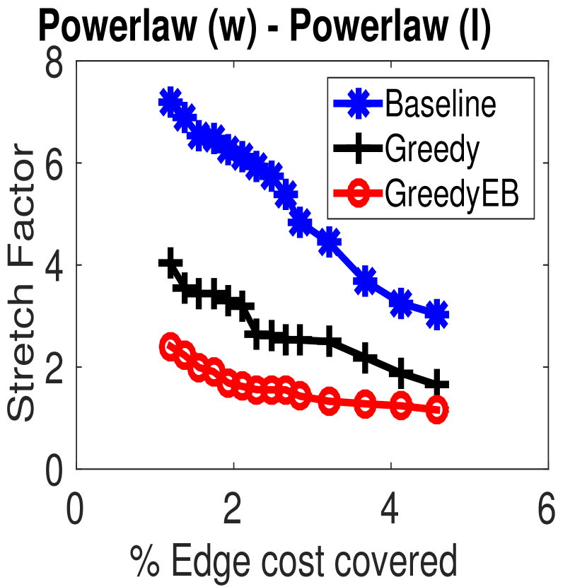
(e)

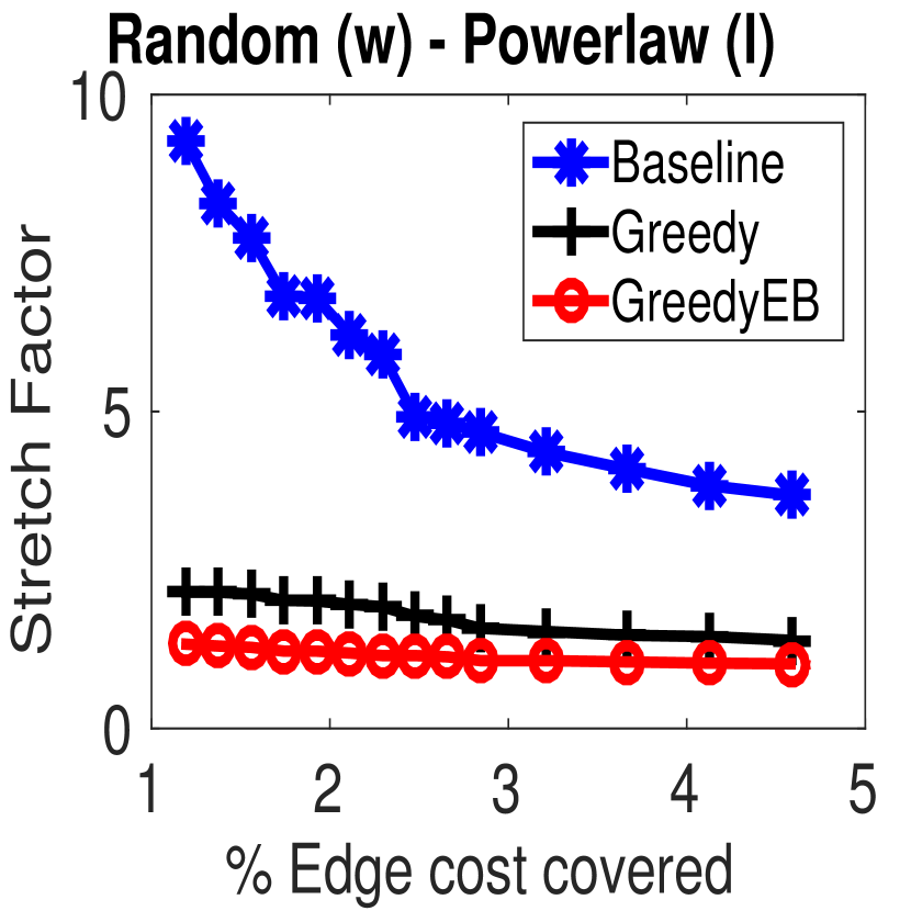
(f)

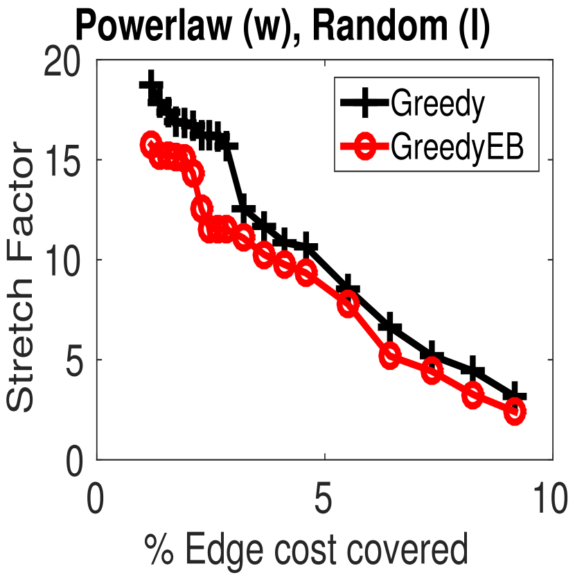
(g)

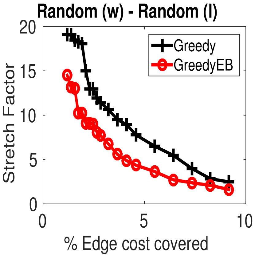
(h)

Figure 4: Effect of edge-betweenness on the performance of the Greedy algorithm, for various datasets (a) LondonTube, (b) USFlights, (c) NYCTaxi, (d) Wikispeedia, (e–h) UKRoad. Baseline is missing in figures (g) and (h) because the stretch factor was very large or infinity. We see a consistent trend that using edge-betweenness improves the performance. In Figures (e–h), $(w)$ indicates traffic volume, and $(l)$ indicates the log.

4.1 Quantitative results.

We focus our evaluation on three main criteria: (i) Comparison of the performance with and without the edge-betweenness measure; (ii) effect of the optimizations, in terms of quality and speedup; and (iii) effect of allocating more budget on the stretch factor.

Effect of edge-betweenness. We study the effect of using edge-betweenness in the Greedy algorithm. The results are presented in Figure 4.

Effect of landmarks. Landmarks provide faster computation with a trade off for quality. Figure 5 shows the speedup achieved when using landmarks. In the figures, BasicGreedyEB indicates the greedy algorithm that doesn’t use any optimizations. GreedyEBCC makes use of the optimizations proposed in Section 3.2 which do not use approximation. GreedyEBLandmarks* makes use of the landmarks optimatization and the * indicates the number of landmarks we tried. Figure 6 shows the performance of GreedyEB algorithm with and without using landmarks.

Budget vs. stretch factor. We examine the trade-off between budget and stretch factor for our algorithm and its variants. A lower stretch factor for the same budget indicates that the algorithm is able to pick better edges for the backbone. Figure 4 shows the trade-off between budget and stretch factor for all our datasets. In all figures the budget used by the algorithms, shown in the $x$-axis, is expressed as a percentage of the total cost of all the edges in the network.

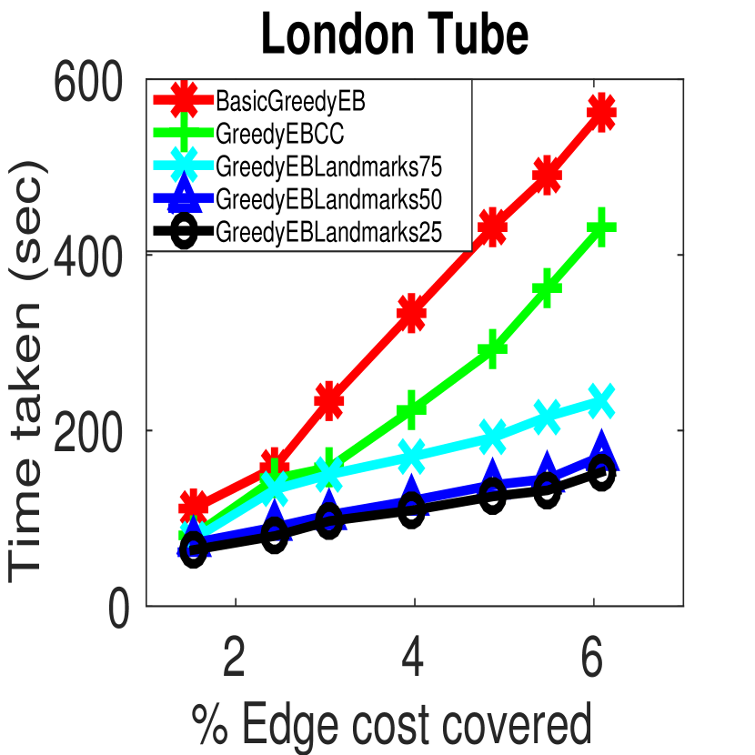
(a)

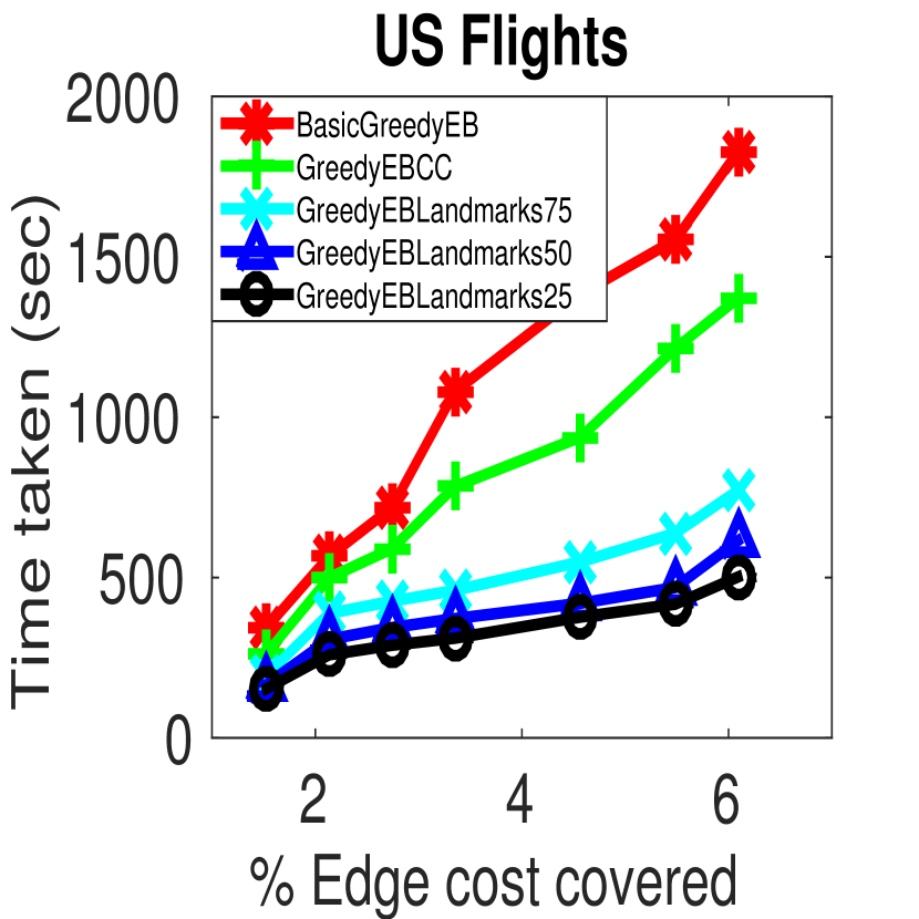
(b)

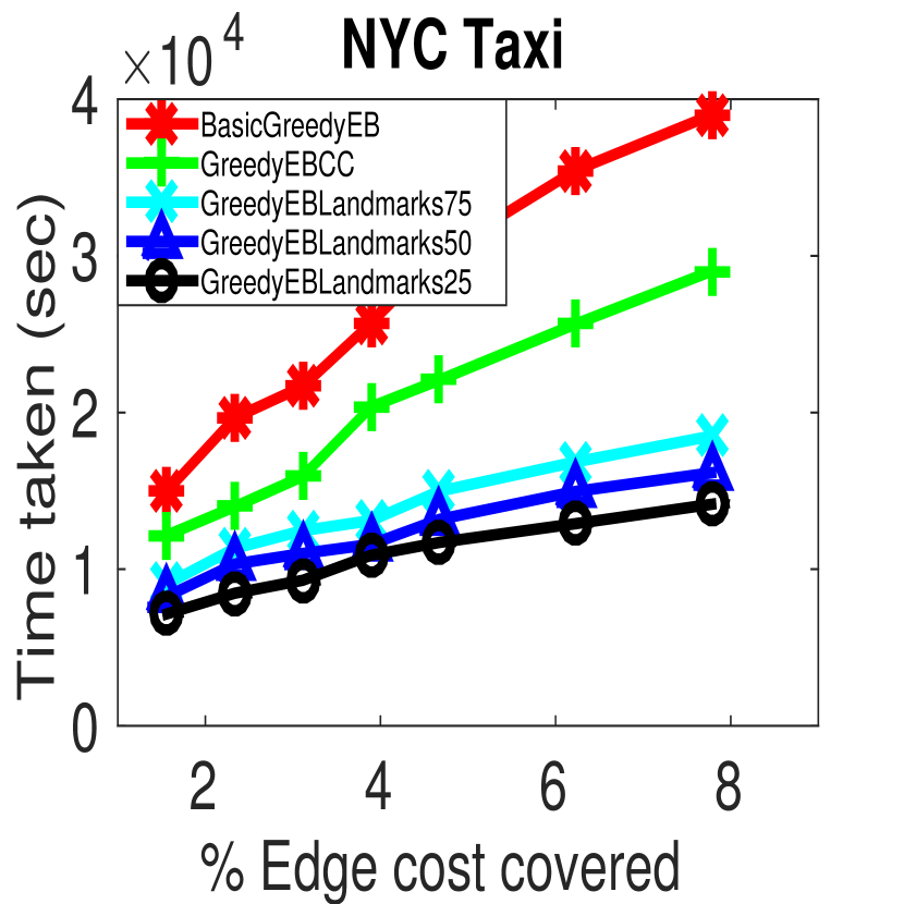
(c)

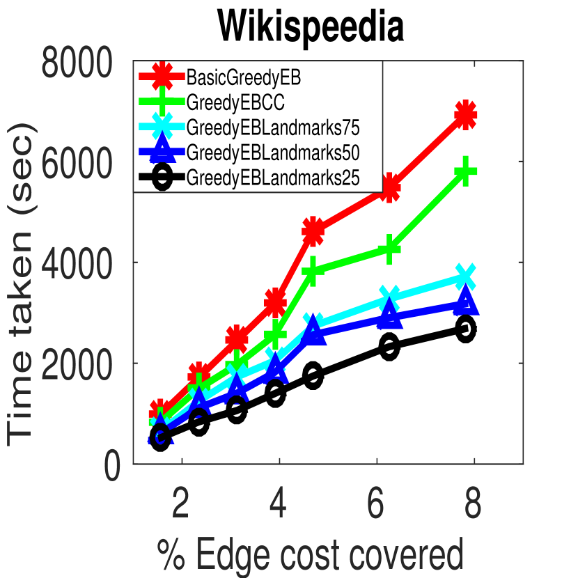
(d)

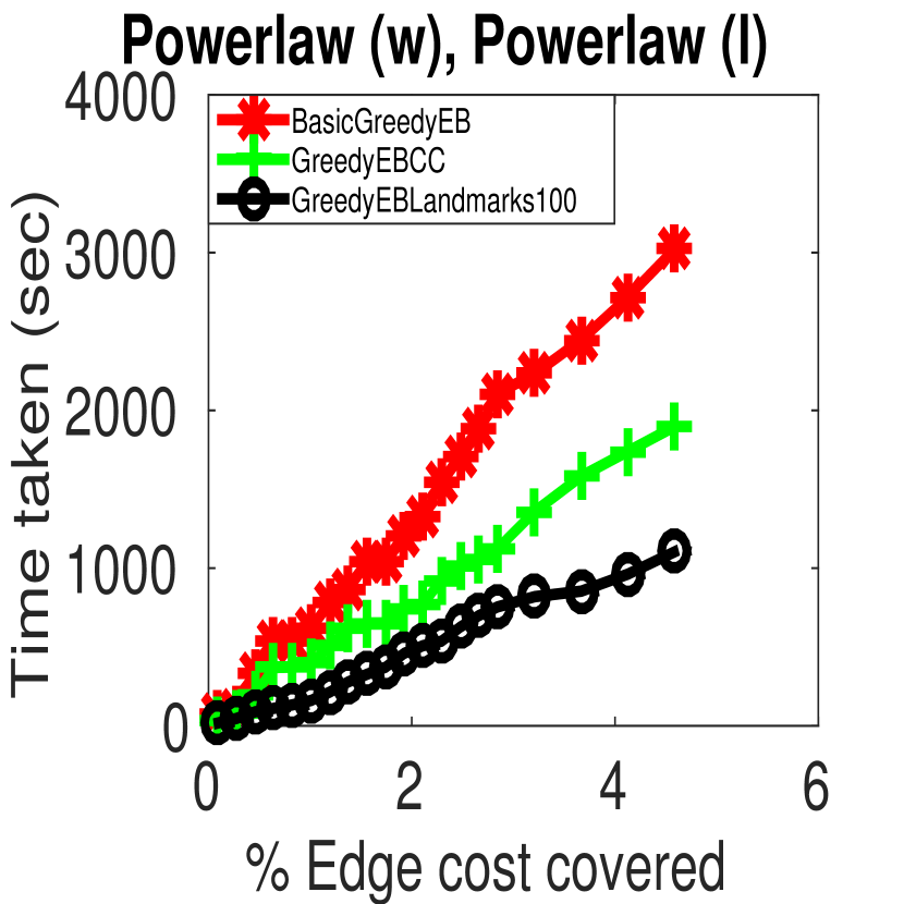
(e)

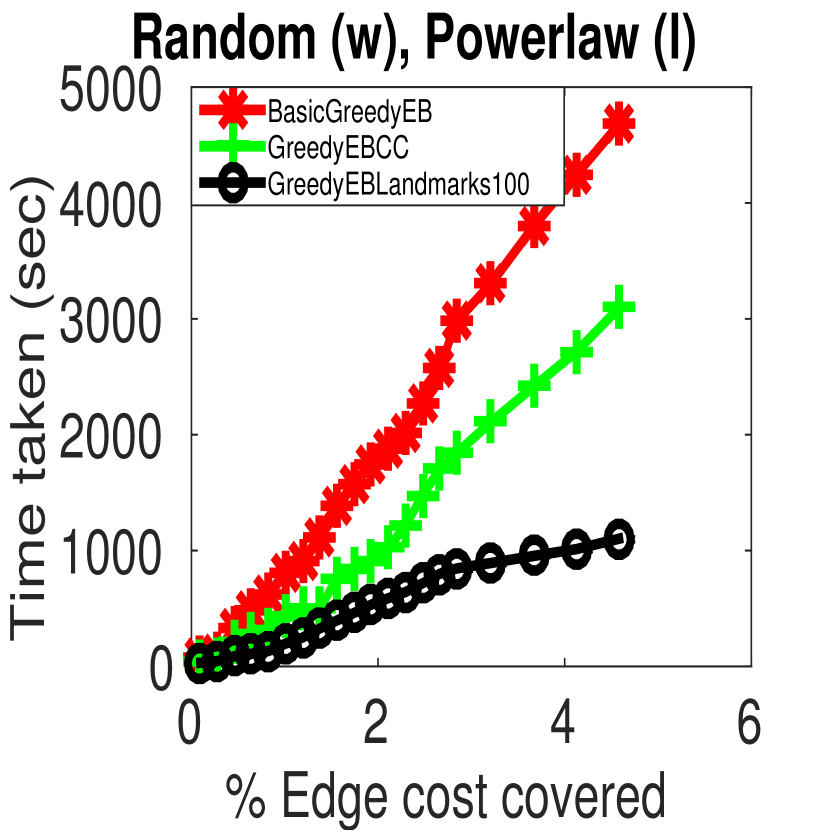
(f)

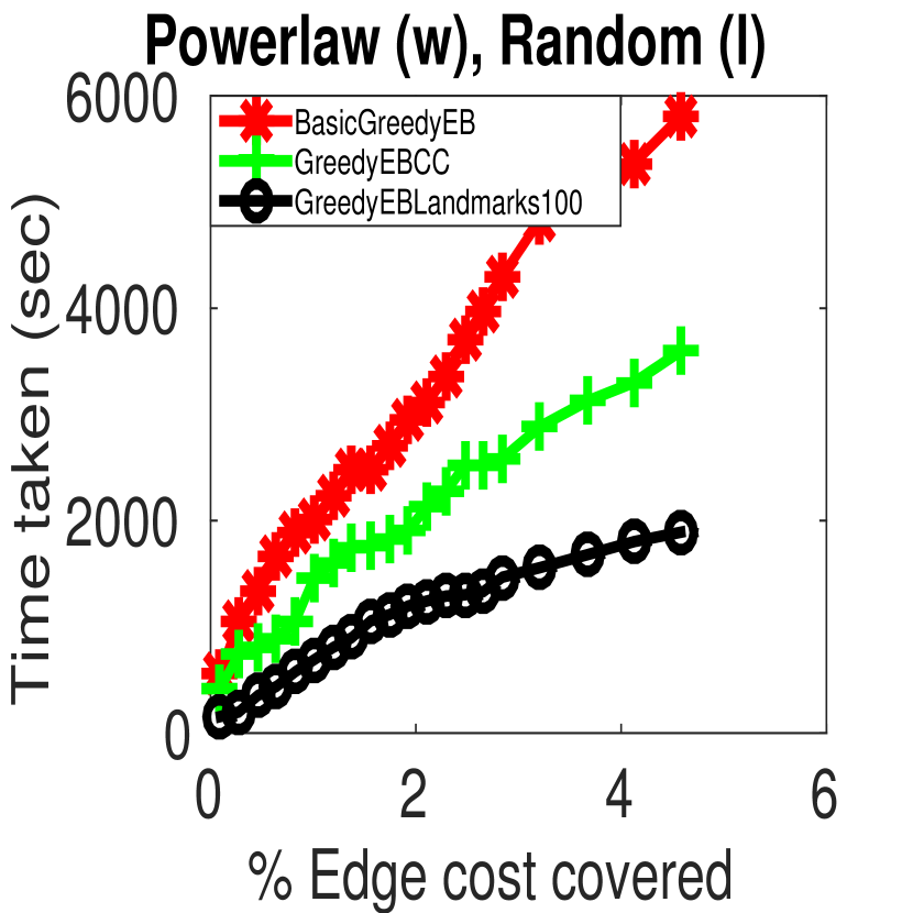
(g)

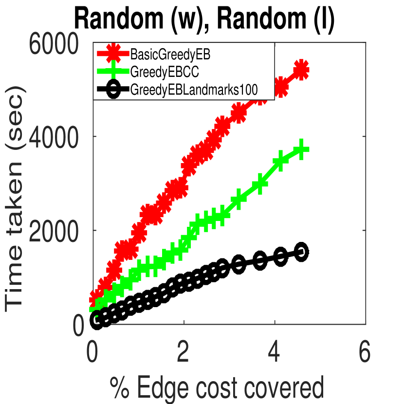
(h)

Figure 5: Comparison of the time taken by the algorithm using different optimizations mentioned in Section 3.2, for (a) LondonTube, (b) USFlights, (c) NYCTaxi, (d) Wikispeedia, (e–h) UKRoad. BasicGreedyEB doesnt use any optimizations, GreedyEBCC is the version using connected components, GreedyEBLandmarks* uses * landmarks. We can clearly see a great improvement (up to 4x) in speed by using landmarks. As we increase the number of landmarks, we trade-off speed with accuracy. In Figures (e–h), $(w)$ indicates traffic volume, and $(l)$ indicates the log.

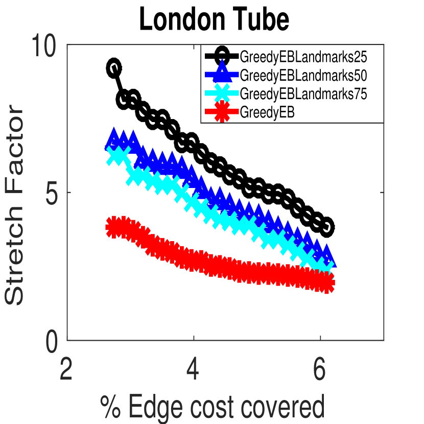
(a)

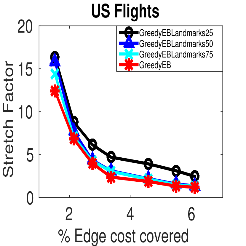
(b)

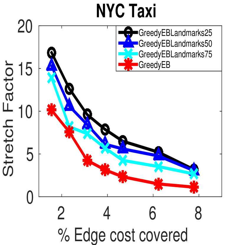
(c)

(d)

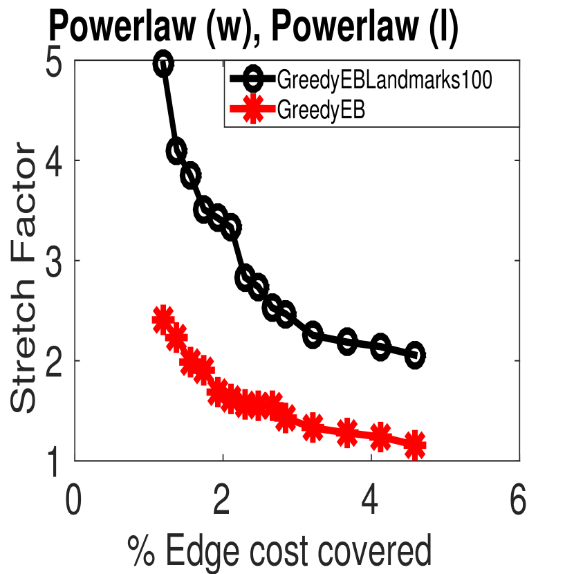
(e)

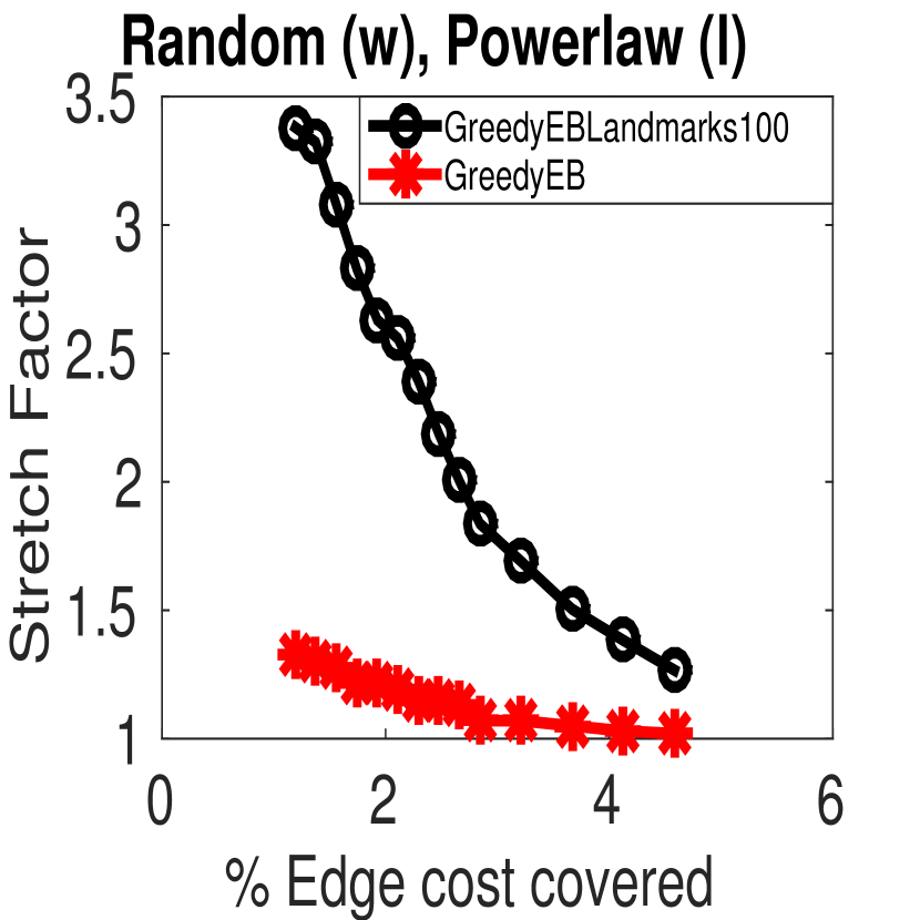
(f)

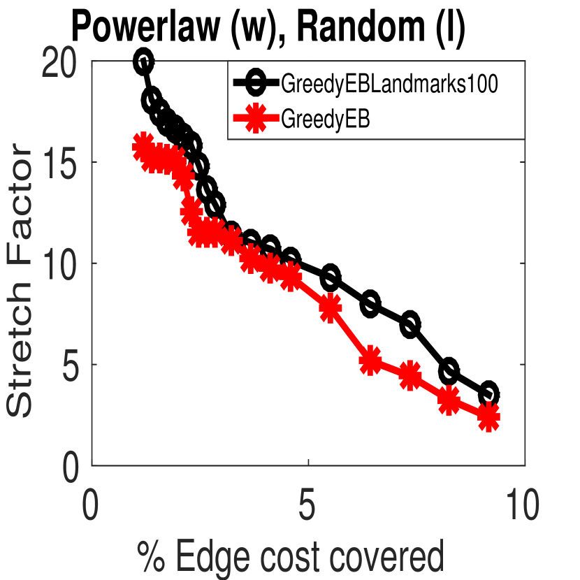
(g)

(h)

Figure 6: Performance in terms of stretch factor of our greedy algorithm with and with out using landmarks, for (a) LondonTube, (b) USFlights, (c) NYCTaxi and (d) Wikispeedia  (e–h) UKRoad. For all the datasets, as expected, we see a slight decrease in performance using landmarks. In Figures (e–h), $(w)$ indicates traffic volume, and $(l)$ indicates the log.

Key findings. From all the above results, we would like to highlight the following points.

1. The greedy algorithm and its variants performs much better than the baseline (See Figure 4). Note that baseline is not included in Figure 4(g,h) because the edges in the baseline are added one-by-one and for a large interval of the cost, the stretch factor was very large or even infinity. This shows that the backbone produced by our greedy approach not only consists of edges with low benefit, but also tries to re-use a lot of edges, hence obtaining a lower stretch factor.

2. The backbones discovered by our algorithms are sparse and summarize well the given traffic (Figures 4, 6). In all cases, with about 15% of the edge cost in the network it is possible to summarize the traffic with stretch factor close to 1. In some cases, even smaller budget (than 15%) is sufficient to reach a lower stretch-factor value.

3. Incorporating edge-betweenness as an edge-weighting scheme in the algorithm improves the performance, in certain cases there is an improvement of at least 50% (See Figure 4; in most cases, even though there is a significant improvement, the plot is overshadowed by a worse performing baseline). This is because, using edges of high centrality will make sure that these edges are included in many shortest paths, leading to re-using many edges.

4. The optimizations we propose in Section 3.2 help in reducing the running time of our algorithm (See Figure 5). For the optimizations not using landmarks, we see around 30% improvement in running time. Using landmarks substantially decreases the time taken by the algorithms (3–4 times). While there is a compromise in the quality of the solution, we can observe from Figures 6 that the performance drop is small in most cases and can be controlled by the choosing the number of landmarks accordingly. Our algorithms, using the various optimizations we propose, are able to scale for large, real-world networks with tens of thousands of nodes which is the typical size of a road/traffic network.

4.2 Comparison to existing approaches

In this section, we compare the performance of BackboneDiscovery with other related work in literature. The comparison is done based on two factors (i) Stretch factor, (ii) Percentage of edges covered by the solution. Intuitively, a good backbone should try to minimize both, i.e. produce a sparse backbone, which also preserves the shortest paths between vertices as well as possible.

Comparison with Prize Collecting Steiner-forest (PCSF) - Prize Collecting Steiner-forest [10] is a variant of the classic Steiner Forest problem, which allows for disconnected source–destination pairs, by paying a penalty. The goal is to minimize the total cost of the solution by ‘buying’ a set of edges (to connect the $s$–$t$ pairs) and paying the penalty for those pairs which are not connected. We compare the performance of our algorithm with PCSF, based on two factors (i) Stretch factor (Figure 7a), (ii) Percentage of edges covered by the solution (Figure 7b). We use the same ($s$,$t$) pairs that we use in our algorithm and set the traffic volume $w_{i}$ as the penalty score in PCSF. We first run PCSF on our datasets and compute the budget of the solution produced. Using the budget as input to our algorithm (GreedyEB), we compute our backbone.

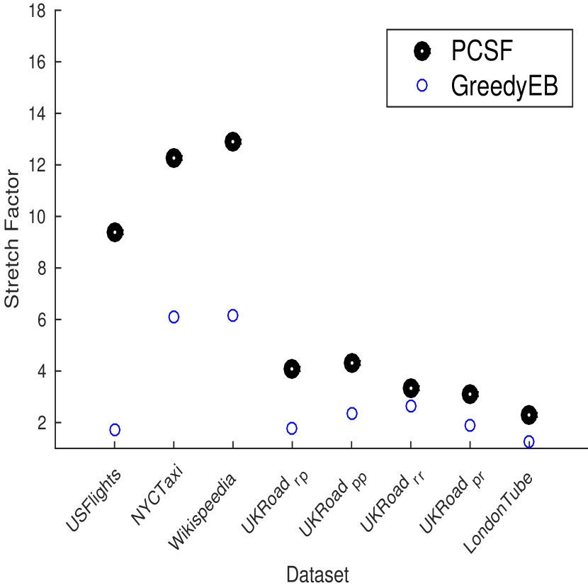
(a)

(b)

Figure 7: Comparison of our algorithm GreedyEB with PCSF, in terms of (a) stretch factor (b) Percentage of edges covered. The 4 variants of UKRoad for the different traffic log are indicated by $UKRoad_{ab}$ where $a$ indicates traffic volume, $b$ indicates (s,t) pairs ($r$ - random, $p$ - powerlaw). (In (b) LondonTube is plotted on a secondary y-axis because of mismatch in scale).

We can see from Figure 7a that our algorithm produces a backbone with a much better stretch factor than PCSF. In most datasets, our algorithm produces a backbone which is at least 2 times better in terms of stretch factor.

Figure 7b compares the fraction of edges covered by our algorithm and PCSF. We observe that the fraction of edges covered by our algorithm is lower than that of PCSF. This could be because our algorithm re-uses edges belonging to multiple paths. Figures 7(a,b) show that even though our solution is much better in terms of stretch factor, we produce sparse backbones (in terms of the percentage of edges covered).

Comparison with k-spanner - As described in Section 5, our problem is similar to $k$-spanner [15] in the sense that we try to minimize the stretch factor. A $k$-spanner of a graph is a subgraph in which any two vertices are at most $k$ times far apart than on the original graph. One of the main advantages of our algorithm compared to spanners is that spanners can not handle disconnected vertices. We also propose and optimize a modified version of stretch factor in order to handle disconnected vertices. Similar to PCSF, we first compute a 2-spanner using a 2 approximation greedy algorithm and compute the budget used. We then run our algorithm for the same budget. Figures 8(a,b) show the performance of our algorithm in terms of stretch factor and percentage of edges covered. Our objective here is to compare the cost our algorithm pays in terms of stretch factor for allowing disconnected vertices. We can clearly observe that even though we allow for disconnected pairs, our algorithm performs slightly better in terms of stretch factor and also produces a significantly sparser backbone.

(a)

(b)

Figure 8: Comparison of our algorithm GreedyEB with 2-spanner in terms of (a) stretch factor (b) Percentage of edges covered.

Comparison with Toivonen et al. [20] - Next, we compare our algorithm with Toivonen, et al [20]. Toivonen et al. propose a framework for path-oriented graph simplification, in which edges are pruned while keeping the original quality of the paths between all pairs of nodes. The objective here is to check how well we perform in terms of graph sparsification. Figures 9(a,b) shows the comparison in terms of stretch factor and percentage of edges covered. Similar to the above approaches, we use the same budget as that used by Toivonen’s algorithm. We observe that for most of the datasets, their algorithm works poorly in terms of sparsification, pruing less than 20% of the edges (Figure 9(b)). Our algorithm performs better both in terms of the stretch of the final solution as well as sparseness of the backbone.

(a)

(b)

Figure 9: Comparison of our algorithm GreedyEB with Toivonen et al, in terms of (a) stretch factor (b) Percentage of edges covered.

The above results, comparing our work with the existing approaches showcase the power of our algoritm in finding a concise representation of the graph, at the same time maintaining a low stretch factor. In all the three cases, our algorithm performs considerably better than the related work.

Fairness - Though we claim that our approach performs better, we need to keep in mind that there might be differences between these algorithms. PCSF does not optimize for stretch factor. Spanners and Toivonen et al. do not have a traffic log (($s$,$t$) pairs). They also do not try to optimize stretch factor. For this section, we were just interested in contrasting the performance of our approach with existing state of the art methods and show how our approach is different and better at what we do.

4.3 Case study #1: NYCTaxi.

The backbone of the NYC taxi traffic, as discovered by our algorithms Greedy and GreedyEB, is shown in Figure 10. We see that both backbones consist of many street stretches in the mid-town (around Times Square) while serving lower-town (Greenwich village and Soho) and up-town (Morningside heights). We also note that there are stretches to the major transportation centers, such as the LaGuardia airport, the World Financial Center Ferry Terminal, and the Grand Central Terminal, as well as to the Metropolitan museum. Comparing the Greedy and GreedyEB backbones, we see that GreedyEB emphasizes more on the traffic to lower-town, and ignores the northern stretch via Robert Kennedy bridge, as it is less likely to be included in many shortest paths. The case study reiterates the advantages of using edge-betweenness to guide the selection of the backbone to include edges which are likely to be used more and is consistent with the well established notion of Wardrop Equilibrium in Transportation Science that users (in a non-cooperative manner) seek to minimize their cost of transportation [21].

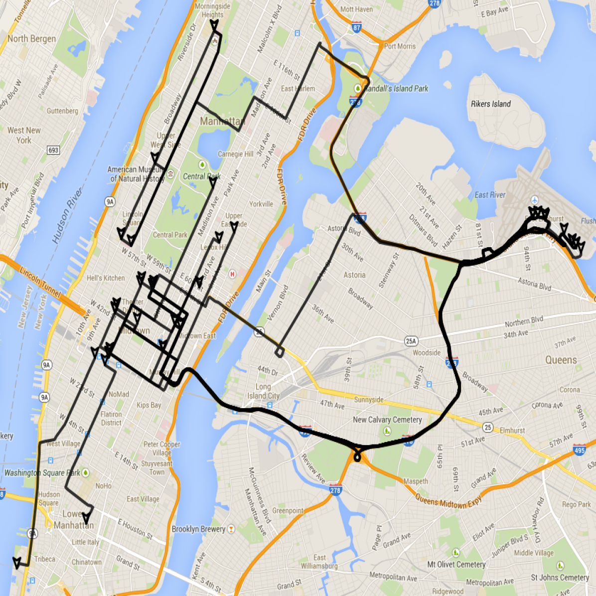
(a)

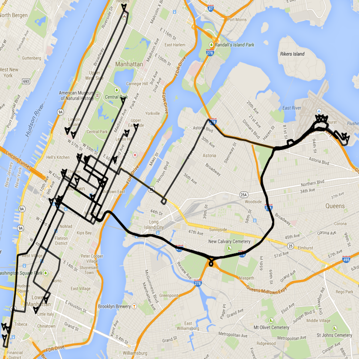
(b)

Figure 10: NYC backbone using (a) Greedy(b) GreedyEB.

4.4 Case study #2: Abeline.

We carry out a qualitative analysis on the Abilene dataset. The results of applying the Greedy algorithm are shown in Figure 11. The results provide preliminary evidence that the backbone produced by our problem can be tightly integrated with software defined networks (SDN), an increasingly important area in communication networks [11]. The objective of SDN is to allow a software layer to control the routers and switches in the physical layers based on the profile and shape of the traffic. This is precisely what our solution is accomplishing in Figure 11. The design of data-driven logical networks will be an important operation implemented through an SDN and will help network designers manage traffic in real time.

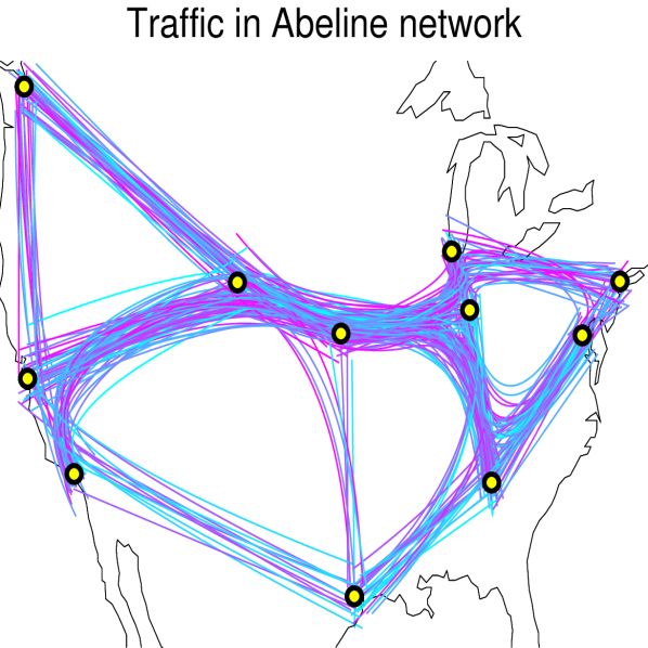
(a)

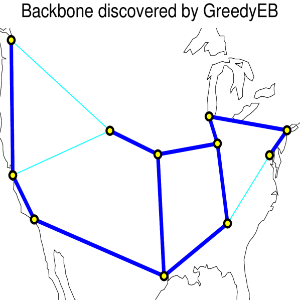
(b)

Figure 11: Qualitative analysis of the real Internet network. The figure on the left shows network traffic in the Abeline dataset, and the one on the right shows the backbone discovered by the GreedyEB algorithm. As in Figure 1, the traffic shown is an interpolation along the shortest path between the source–destination pairs.

5 Related work

As already noted, BackboneDiscovery is related to the $k$-spanner and the Steiner-forest problem and the decision versions of both are known to be $\mathbf{NP}$-complete [15, 23]. The $k$-spanner problem is designed to bound the stretch factor for all pairs of nodes and not just those from a specific set of $(s,t)$ pairs. The Steiner-forest problem on the other hand is designed to keep the $(s,t)$ pairs connected with a minimal number of edges and is agnostic about the stretch factor. Both these problems only consider structural information and completely ignore functional (activity) data that maybe available about the usage of the network. They also have strict limitations that all nodes need to be covered, which makes them restrictive.

The Prize collecting Steiner-forest problem (PCSF) [10] is a version of the Steiner-forest problem that allows for disconnected source–destination pairs, by imposing a penalty for disconnected pairs. Even in this variant, there is no budget or stretch requirement and hence the optimization problem that PCSF solves is completely different from what we solve. We show how our algorithm fares in comparison to PCSF in Section 4.2.

Another enhancement in our work is to normalize edge costs with measures related to the structure of the network (like edge betweenness [3, 9, 16]) As we show in our experiments, this leads to finding solutions of better quality.

Our work is different from trajectory mining [8, 24], which consider complete trajectories between source–destination pairs. We do not make use of the trajectories and are only interested in the amount of traffic flowing between a source and destination. Also, the type of questions we try to answer in this paper are different from that of trajectory mining. While trajectory mining tries to answer questions like “Which are the most used routes between A and B?”, our paper tries to use information about traffic from A to B in order to facilitate a sparse backbone of the underlying network which allows traffic to flow from A to B, also keeping global network characteristics in mind.

The BackboneDiscovery problem is also related to finding graph sparsifiers and simplifying graphs. For example, Toivonen et al. [20] as well as Zhou et al [25], propose an approach based on pruning edges while keeping the quality of best paths between all pairs of nodes, where quality is defined on concepts such as shortest path or maximum flow. Misiolek and Chen [14] propose an algorithm which prune edges while maintaining the source-to-sink flow for each pair of nodes. Mathioudakis et al. [13] and Bonchi et al. [2] study the problem of discovering the backbone of a social network in the context of information propagation, which is a different type of activity than source–destination pairs, as considered here. In the work of Butenko et al. a heuristic algorithm for the minimum connected dominating subset of wireless networks was proposed [4]. There has been some work in social network research to extract a subgraph from larger subgraphs subject to constraints [7, 19]. Other forms of network backbone-discovery have been explored in domains including biology, communication networks and the social sciences. The main focus of most of these approaches is on the trade-off between the level of network reduction and the amount of relevant information to be preserved either for visualization or community detection. While in this paper we try to also sparsify a graph, our objective and approach is completely different from the above because we cast the problem in a well-defined optimization framework where the structural aspects of the network are captured in the requirement to maintain a low stretch while the functional requirements are captured in maintaining connectedness between traffic terminals, which has not been done before.

In the computer network research community, the notion of software defined networks (SDN), which in principle decouples the network control layer from the physical routers and switches, has attracted a lot of attention [5, 11]. SDN (for example through OpenFlow) will essentially allow network administrators to remotely control routing tables. The BackboneDiscovery problem can essentially be considered as an abstraction of the SDN problem, and as we show in Section 4.4, our approach can make use of traffic logs to help SDN’s make decisions on routing and switching in the physical layer.

6 Conclusions

We introduced a new problem, BackboneDiscovery, to address a modern phenomenon: these days not only is the structural information of a network available but increasingly, highly granular functional (activity) information related to network usage is accessible. For example, the aggregate traffic usage of the London Subway between all stations is available from a public website. The BackboneDiscovery problem allowed us to efficiently combine structural and functional information to obtain a highly sophisticated understanding of how the Tube is used (See Figure 1). From a computational perspective, the BackboneDiscovery problem has elements of both the $k$-spanner and the Steiner-forest problem and thus requires new algorithms to maintain low stretch and connectedness between important nodes subject to a budget constraint. We compare our algorithm with other similar algorithms and show how our algorithm is different and performs better for our setting. Our case studies show the application of the proposed methods for a wide range of applications, including network and traffic planning.

Though our algorithm makes use of shortest paths, in practice, any other types of paths could be incorporated into our algorithm. We leave this generalization for future analysis. The use of harmonic mean not only allows us to handle disconnected (s,t)-pairs, but also makes our stretch factor measure more sensitive to outliers. For future work, we would also incorporate a deeper theoretical analysis of the algorithm and the stretch factor measure.

References

- [1] P. Boldi and S. Vigna. Axioms for centrality. CoRR, abs/1308.2140, 2013.
- [2] F. Bonchi, G. De Francisci Morales, A. Gionis, and A. Ukkonen. Activity preserving graph simplification. DMKD, 27(3), 2013.
- [3] U. Brandes and C. Pich. Centrality estimation in large networks. IJBC, 17(7), 2007.
- [4] S. Butenko, X. Cheng, C. A. Oliveira, and P. M. Pardalos. A new heuristic for the minimum connected dominating set problem on ad hoc wireless networks. Cooperative Systems, 3, 2004.
- [5] M. Casado, M. J. Freedman, J. Pettit, J. Luo, N. Gude, N. McKeown, and S. Shenker. Rethinking enterprise network control. IEEE/ACM Trans. Netw., 17(4):1270–1283, 2009.
- [6] A. Das Sarma, S. Gollapudi, M. Najork, and R. Panigrahy. A sketch-based distance oracle for web-scale graphs. In WSDM, 2010.
- [7] N. Du, B. Wu, and B. Wang. Backbone discovery in social networks. Web Intelligence, 2007.
- [8] F. Giannotti, M. Nanni, F. Pinelli, and D. Pedreschi. Trajectory pattern mining. In Proceedings of the 13th ACM SIGKDD international conference on Knowledge discovery and data mining, pages 330–339. ACM, 2007.
- [9] M. Girvan and M. Newman. Community structure in social and biological network. PNAS, 2002.
- [10] M. Hajiaghayi, R. Khandekar, G. Kortsarz, and Z. Nutov. Prize-collecting steiner network problems. In Integer Programming and Combinatorial Optimization, pages 71–84. Springer, 2010.
- [11] H. Kim and N. Feamster. Improving network management with software defined networking. IEEE Communications Magazine, 51(2):114–119, 2013.
- [12] M. Marchiori and V. Latora. Harmony in the small world. Physica A, 285, 2000.
- [13] M. Mathioudakis, F. Bonchi, C. Castillo, A. Gionis, and A. Ukkonen. Sparsification of influence networks. In KDD, 2011.
- [14] E. Misiolek and D. Z. Chen. Two flow network simplification algorithms. IPL, 97, 2006.
- [15] G. Narasimhan and M. Smid. Geometric Spanner Networks. Cambridge University Press, 2007.
- [16] M. Newman. A measure of betweenness centrality based on random walks. Social Networks, 27, 2005.
- [17] M. Newman and M. Girvan. Finding and evaluating community structure in networks. Phys. Rev., 69, 2004.
- [18] M. Potamias, F. Bonchi, C. Castillo, and A. Gionis. Fast shortest path distance estimation in large networks. In CIKM, 2009.
- [19] N. Ruan, R. Jin, G. Wang, and K. Huang. Network backbone discovery using edge clustering. arXiv:1202.1842, 2012.
- [20] H. Toivonen, S. Mahler, and F. Zhou. A framework for path-oriented network simplification. In IDA, 2010.
- [21] J. Wardrop and J. Whitehead. Correspondence. some theoretical aspects of road traffic research. In ICE:Engineering Divisions, page 767, 1952.
- [22] R. West, J. Pineau, and D. Precup. Wikispeedia: An online game for inferring semantic distances between concepts. In IJCAI, pages 1598–1603, 2009.
- [23] D. Williamson and D. Shmoys. The Design of Approximation Algorithms. CUP, 2011.
- [24] Y. Zheng, L. Zhang, X. Xie, and W.-Y. Ma. Mining interesting locations and travel sequences from gps trajectories. In Proceedings of the 18th international conference on World wide web, pages 791–800. ACM, 2009.
- [25] F. Zhou, S. Mahler, and H. Toivonen. Network simplification with minimal loss of connectivity. In IDA, 2010.