Multiwavelength modelling the SED of supersoft X-ray sources
II. RS Ophiuchi: From the explosion to the SSS phase

Abstract

RS Oph is a recurrent symbiotic nova that undergoes nova-like outbursts on a time scale of 20 years. Its two last eruptions (1985 and 2006) were subject of intensive multiwavelengths observational campaign from the X-rays to the radio. This contribution aims to determine physical parameters and the ionization structure of the nova from its explosion to the first emergence of the supersoft X-rays (day 26) by using the method of multiwavelength modelling the SED. From the very beginning of the eruption, the model SED revealed the presence of both a strong stellar and nebular component of radiation in the spectrum. During the first 4 days, the nova evinced a biconical ionization structure. The $\sim 8200$ K warm and 160–200 $R_{\odot}$ extended pseudophotosphere encompassed the white dwarf (WD) around its equator to the latitude $>40^{\circ}$. The remaining space around the WD’s poles was ionized, producing a strong nebular continuum with the emission measure $\textsl{EM}\sim 2.3\times 10^{62}$ cm^-3 via the fast wind from the WD. The luminosity of the burning WD was highly super-Eddington for the whole investigated period. The wind mass loss at rates of $10^{-4}-10^{-5}$ $M_{\odot}\,{\rm yr}^{-1}$ and the presence of jets suggest an accretion throughout a disk at a high rate, which can help to sustain the super-Eddington luminosity of the accretor for a long time.

H I G H L I G H T S

• Physical parameters of the nova RS Oph were determined from its X-ray/IR spectrum.

• The model revealed the presence of a strong stellar and nebular component.

• The luminosity was super-Eddington during the whole burning phase.

• The high luminosity was sustained by a super-critical accretion.

1 Introduction

The star RS Ophiuchi (RS Oph) is located in the direction nearby to the galactic center ($l_{\rm II}=+19^{\circ}.8~{}b_{\rm II}=+10^{\circ}.4$) at a distance $d=1.6\pm 0.3\,{\rm kpc}$ (Hjellming et al., 1986; Bode, 1987; Barry et al., 2008a). The light of RS Oph is significantly attenuated by interstellar extinction. Hjellming et al. (1986) determined from H I 21 cm measurements the interstellar absorbing column, $N_{\rm H}=(2.4\pm 0.3)\times 10^{21}$  cm^-2, and Snijders (1987) derived the color excess $E_{\rm B-V}=0.73\pm 0.1$ mag from ultraviolet IUE spectra. According to the relationship between $N_{\rm H}$ and $E_{\rm B-V}$ (e.g. Diplas & Savage, 1994), both these parameters are consistent.

RS Oph is a recurrent symbiotic nova comprising a late-type, K7 III, giant (Mürset & Schmid, 1999) and a WD with a mass close to the Chandrasekhar limit (e.g. Bode, 1987, and references therein), in a 456-day orbit (Fekel et al., 2000; Brandi et al., 2009). Its nova-like outbursts are characterized with brightening by about 7 mag and a recurrence period of about 20 years. Historically, 6 eruptions have been recorded unambiguously. The first one in 1898 and the last one on 2006 February 12.83 (Evans et al., 1988; Narumi et al., 2006). The recurrence period of approximately 20 years and a bright peak magnitude, $V=4-5$, made RS Oph a good target for multifrequency observational campaigns (e.g. Evans et al., 2007, and references therein).

At the beginning of the last two outbursts of 1985 and 2006, observations revealed a non-spherical shape of the nova ejecta, (i) on the radio maps (e.g. Taylor et al., 1989; O’Brien et al., 2006; Rupen et al., 2008; Sokoloski et al., 2008), (ii) by interferometric technique in the near and mid-IR (e.g. Monnier et al., 2006; Lane et al., 2007; Chesneau et al., 2007; Barry et al., 2008b), (iii) by the HST imaging in the optical (Bode et al., 2007), (iv) by the Chandra X-ray Observatory detected as an extended X-ray emission elongated in the line with the extended infrared emission (Luna et al, 2009) and (v) by the asymmetric line profiles measured on day 13.9, interpreted by Drake et al. (2009) as a result of the shock collimation due to equatorial circumstellar density enhancement. Particularly, highly collimated jet-like ejection was indicated by the optical spectroscopy during the first 30 days after the eruption (Skopal et al., 2008a; Banerjee et al., 2009).

The 2006 outburst was intensively monitored with the Swift and the Rossi X-ray Timing Explorer. Prior to day 26, the behaviour of the X-ray flux was described by the evolution of shock systems established as the high-velocity ejecta impacted the red giant wind (Bode et al., 2006; Sokoloski et al., 2006). The evolving shock in the 2006 outburst of RS Oph was analyzed in detail by Ness et al. (2009) using the high-resolution X-ray grating observations with Chandra and XMM-Newton. The X-ray observations demonstrated that the supersoft X-ray phase of nova RS Oph started rapidly from day 26 (see also Osborne et al., 2011).

The detailed spectral evolution of the 2006 outburst in the optical was reported by Iijima (2009). He suggested that the profiles of the prominent emission lines resulted from a rapidly expanding ($\sim 1000$ km s^-1), low density part and a slowly moving ($\sim 100$ km s^-1) high density part in the ejecta, which are probably related to the expansion along the polar and the equatorial regions, respectively.

In this contribution I aim to determine physical parameters of the nova RS Oph from its explosion to the first emergence of the supersoft X-rays (day 26) by using the method of multiwavelength modelling the SED. Based on the results from spectral fits, I also explore the ionization structure of the nova during the first 4 days of its outburst. Section 2 introduces multi-band observations at selected days, and the results of their SED-fitting analysis are given in Sect. 3. Discussion and summary are found in Sects. 4 and 5, respectively.

2 Observations

To map the evolution of the fast nova RS Oph by the multiwavelength approach, simultaneous observations covering a large wavelength range, taken at different days after the explosion, are required. Rapid changes in the SED following the blast require frequent sets of observations. According to these conditions, it was possible to select (near-)simultaneous observations at/around day 1, 3.8, 7.3, 14.6, 19.5 and 26 after the optical maximum of the RS Oph outburst. Selection of the appropriate data benefited from a strong similarity of the recent 1985 and 2006 outbursts in the supersoft X-ray, optical and near-IR light curve profiles (e.g. Ness et al., 2007; Rosino, 1987; Banerjee et al., 2009). Therefore, observations taken at the same time after the optical maximum of these outbursts were assumed to be simultaneous.

The UV to near-IR observations were dereddened with $E_{\rm B-V}$ = 0.73 and the resulting parameters were scaled to the distance of 1.6 kpc (see Sect. 1). The log of the used observations is given in Table 1.

Table 1: Log of observations

Julian date	Daya	Region	Observatory / (ref.)
2 453779.97	0.64	$J,H$	private / (1)
2 453779.99	0.66-	$B,V,R_{\rm C},I_{\rm C}$	private / (2)
2 453780.71	-1.38	$-$	private / (2)
2 453780.97	1.64	$J,H$	private / (1)
2 453780.33	1	$J,H,K,L$	SAAOb,Mt. Abub/ (3)
2 453780.40	1.07	350–920 nm	HCT, VBT/ (4)
2 453783.13	3.8	8.06–12.26 $\mu$m	Keck N-band/ (5)
2 453783.33	3-4	350–930 nm	HCT, VBT/ (4)
2 453783.13	3.8	$B,V,R_{\rm C},I_{\rm C}$	VSOLJc
2 453783.13	3.8	$J,H,K,L$	SAAOc,Mt. Abuc/ (3)
2 446099.30	7.33	115–335 nm	IUE
2 446099.30	7.33	$UVI_{C}HKL$	SAAOc
2 446106.61	14.6	115–335 nm	IUE
2 446106.61	14.6	$UVI_{C}HKL$	SAAOc,Mt. Abuc/ (3)
2 446111.51	19.5	115–335 nm	IUE
2 446111.51	19.5	$UVI_{C}HKL$	SAAOc,Mt. Abuc/ (3)
2 453805.53	26.20	0.65–3.1 nm	XMM-Newton
2 446117.96	25.99	115–335 nm	IUE
2 446117.96	25.99	$UVI_{C}JHKL$	SAAOc

^a = JD – JD_max (JD_max 2 446 091.97 as on 1985 Jan. 26.47;
                     JD_max 2 453 779.33 as on 2006 Feb. 12.83)
^b values extrapolated to day 1
^c values interpolated to the given day
1 - West (2006), 2 - Sostero & Guido (2006) and VSOLJ observers (see Fig. 1), 3 - Evans et al. (1988); Banerjee et al. (2009), 4 - Anupama (2008), 5 - Barry et al. (2008b).

2.1 Observed SED of the giant

Radiation of the giant in RS Oph can be measured directly only during the quiescent phases. The preliminary model SED showed that the giant dominates the spectrum from the V passband to longer wavelength during the post-outburst minimum (see Fig. 1 of Skopal et al., 2008a, day 253). Therefore, the giant’s continuum was approximated by the photometric $VR_{C}I_{C}$ fluxes from the 2006 post-outburst minimum (the data were collected by the VSOLJ observers, Kiyota, Kubotera, Maehara and Nakajima), $JHKL$ flux-points obtained during 1986 quiescence (Evans et al., 1988) and the archival $ISO$ spectrum from 23/09/1996 which determines the region between 2.3 and 4.0 $\mu$m. Some representative fluxes were taken from the infrared (0.8–5 $\mu$m) spectra obtained during 2006 August to 2008 July (see Fig. 6 of Rushton et al., 2010).

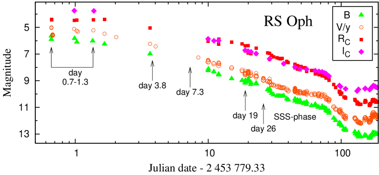
Figure 1: The $BVR_{C}I_{C}$ light curves of RS Oph from its optical maximum (2006 February 12.83) to the quiescent phase (d$>100$). Arrows denote times with reconstructed SEDs (Table 1, Fig. 3). The data were collected by the VSOLJ observers, Kiyota, Kubotera, Maehara and Nakajima.

2.2 Day 0.7–1.4

Observations at the very beginning stage of the nova outburst were restricted to $B,V,R_{C},I_{C}$ flux-points measured between day 0.66 and 1.37 (Sostero & Guido, 2006) and $J$ and $H$ magnitudes obtained by West (2006) at day 0.64 and 1.64 after the optical maximum of the 2006 outburst. In addition, fluxes derived from $K$ and $L$ magnitudes, obtained by linear extrapolation of the data measured at day 8.68, 9.65, 15.65 by Evans et al. (1988) and at day 11.12, 15.09, 17.12 by Banerjee et al. (2009) to day 1, were used.

2.3 Day 3.8

Approximately 3.8 days following the 2006 outburst, RS Oph was observed using the Keck Interferometer Nuller (KIN), which operates in $N$ band from 8 to 12.5 $\mu$m (Barry et al., 2008b). Corresponding fluxes, used in this paper, represent the light from the entire region detected by the KIN in its inner and outer spatial regime (Barry, private communication). At/around day 4, on 2006 February 16, a low resolution spectrum ($R\sim 1000$) covering the range between 350 and 920 nm was obtained at the Indian Astronomical Observatory with the 2-m Himalayan Chandra Telescope (Anupama, 2008). The spectrum is available at. For the purpose of this paper we used its short wavelength part covering the Balmer jump. We calibrated the spectrum to absolute fluxes with the aid of the simultaneous photometric observations. Photometric $B,V,R_{C},I_{C}$ magnitudes were collected by the VSOLJ observers. Flux in the $I_{C}$ band was estimated by the interpolation to day 3.8 (see Fig. 1). The near-IR $J$ and $H$ photometric fluxes at day 3.8 were obtained by linear interpolation of the values published by West (2006), Evans et al. (1988) and Banerjee et al. (2009). The $K$ and $L$ magnitudes were obtained by the same way as described in Sect. 2.2, but extrapolating the measured values to day 3.8.

2.4 Days 7.3–19.5

The first ultraviolet spectra od RS Oph were taken at day 7.3 by the IUE satellite (1985 February 2). We used the spectra SWP25152 and LWP05277, exposed in the low dispersion mode using the large aperture. The LWP05277s spectrum, which was taken with the small aperture, was used to fill in the saturated part of the large aperture spectrum. The small aperture spectrum was multiplied by a factor of 2.2 to match the large aperture one. The following IUE spectra exposed in both primes were made on 1985 February 10, at day 14.6 (SWP25209, LWP5335-6). The last set of the well exposed IUE spectra, without measured SSS X-ray counterpart, was obtained at day 19.55 (SWP25246, LWP05367). The spectra were complemented with the $UVI_{C}HKL$ fluxes, derived from the photometric measurements (Evans et al., 1988; Banerjee et al., 2009, and Fig. 1).

2.5 Day 26

The first detection of supersoft X-ray emission was made by the X-Ray Telescope (0.3–10 keV) onboard the Swift satellite on day 26.0 (see Fig. 3 of Osborne et al., 2011) and by the XMM-Newton satellite, 26.1 days after the 2006 eruption (see Fig. 1 of Ness et al., 2009). Simultaneously, at day 26.0 after the optical maximum of the 1985 outburst, the ultraviolet spectra (SWP25289, LWP05403) were obtained by the IUE satellite. Spectroscopic observations were complemented with the $UVI_{C}JHKL$ photometric fluxes as in previous cases. Fluxes derived from $B$ and $R_{C}$ magnitudes were not used in the modelling the continuum SED, because of a strong saturation with emission lines (see Skopal, 2007).

The X-ray-grating spectrum (RGS1) was extracted using the standard tools provided by the mission-specific software packages (Hanke, private communication). The spectrum was described by Nelson et al. (2008) in detail. To correct the observed X-ray fluxes for absorptions, the tbabs absorption model for ISM composition with abundances given by Wilms et al. (2000) (e.g. $\log(A_{\rm OI})+12=8.69$) was used.

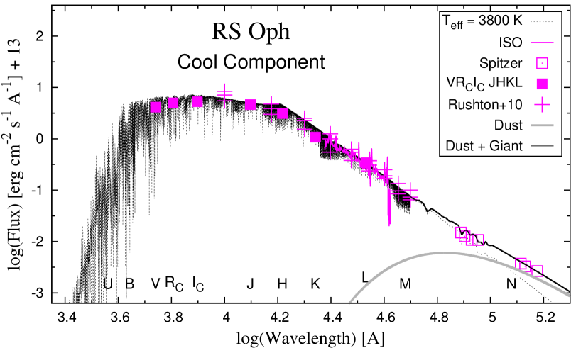
Figure 2: The observed SED of the giant in RS Oph (in violet) compared with an atmospheric model calculated for $T_{\rm eff}=3800$ K (dotted line). A weak blackbody radiating at $\sim 450$ K is required to fit the continuum around the $N$ band (data from Barry et al., 2008b).

3 Results of the SED-fitting analysis

In this section I describe modelling the observed SEDs at the selected days after the optical maximum (Sect. 2). The fitting analysis was performed in the same way as introduced by Skopal (2014, Paper I). The best solution was selected from a grid of model parameters, which corresponded to a minimum of a standard $\chi^{2}$ function. Also in this paper, typical errors in the measured fluxes of $\sim 10$% were adopted. Because of the presence of the giant in the binary, the spectrum $F(\lambda)$ emitted by RS Oph was disentangled into three components,

$$F(\lambda)=F_{\rm h}(\lambda)+F_{\rm n}(\lambda)+F_{\rm g}(\lambda),$$ (1)

where $F_{\rm h}(\lambda)$ is the flux produced by the WD pseudophotosphere, $F_{\rm n}(\lambda)$ is the nebular component from thermal plasma and $F_{\rm g}(\lambda)$ represents the contribution from the giant. They are defined in Paper I. To simplify the task, we first estimated the contribution from the giant using observations made during quiescent phase (Sect. 2.1). Then, assuming that the giant’s radiation is constant, its contribution was subtracted from the observed fluxes. Resulting model SEDs are depicted in Figs. 2 and 3, and the corresponding parameters are collected in Table 2.

3.1 Radiation characteristics and radius of the giant

Empirical relations between the spectral type (K7 III, Sect. 1) and effective temperature ($T_{\rm eff}$) for cool giants suggest $T_{\rm eff}\sim 4000$ K and a linear radius $R_{\rm g}\sim 50$ $R_{\odot}$ for the giant in RS Oph (e.g. van Belle et al., 1999).

According to the surface brightness relation for M-giants (Dumm & Schild, 1998), the reddening-free magnitudes from the 1986 quiescence, ($J$ = 7.09 and $K$ = 6.41 mag, Evans et al., 1988) yield the angular radius of the giant $\theta_{\rm g}=R_{\rm g}/d=7.0\times 10^{-10}$, i.e. $R_{\rm g}=50\,(d/1.6\,{\rm kpc})$ $R_{\odot}$.

Modelling the infrared spectra of RS Oph, taken during its quiescent phase (2006 August – 2008 July), Pavlenko et al. (2008) and Rushton et al. (2010) determined the effective temperature of the giant $T_{\rm eff}=4100\pm 100$ K and $4200\pm 200$ K, respectively.

Using our approach (see Sect. 2.5 in Paper I), the observed SED of the giant (550–5000 nm, Sect. 2.1) can be compared with the synthetic spectra (models from Hauschildt et al., 1999, Fig. 2 here) with limiting $T_{\rm eff}$ = 3800 and 4000 K, which are scaled with the angular radius of the giant, $\theta_{\rm g}=R_{\rm g}/d$ = 8.6 and $7.7\times\,10^{-10}$, respectively (see Eq. (10) in Paper I). These couples of parameters define the observed bolometric flux $F_{\rm g}^{\rm obs}=\theta_{\rm g}^{2}\sigma T_{\rm eff}^{4}=(8.7\pm 1.2)\times 10^{-9}$ $\,\rm erg\,cm^{-2}\,s^{-1}$, where the uncertainty represents that in the observed fluxes ($\sim 15$%). The distance $d$ converts this quantity to the luminosity of the giant $L_{\rm g}=(690\pm 95)\,(d/1.6\,{\rm kpc})^{2}$ $L_{\odot}$, and $\theta_{\rm g}$ to the radius of the giant $R_{\rm g}=(61-55)\,(d/1.6\,\,{\rm kpc})$ $R_{\odot}$. Figure 2 compares the model for $T_{\rm eff}$ = 3800 K and $\theta_{\rm g}=8.6\times\,10^{-10}$.

The giant underfills its Roche lobe for the distance of 1.6 kpc. The orbital solution for both components of the binary (Brandi et al., 2009) and the WD mass of 1.3 $M_{\odot}$ yield the Roche lobe radius of the giant $\sim 110$ $R_{\odot}$, which is a factor of $\sim 2$ larger than $R_{\rm g}$ (see also Sect 4.7 in the following paper, RS Ophiuchi: The supersoft X-ray phase and beyond).

3.2 Optical maximum: The first day

The reconstructed SED from around day 1 covers the range of 0.44–3.4 $\mu$m (Sect. 2.2). Fitting these data revealed the presence of two strong radiative contributions within this domain. A stellar-type component from the inflated WD’s pseudophotosphere and that from thermal nebula. The former dominated the SED within the $B,V,R_{C},I_{C},J,H$ passbands, while the latter was larger within the $K$ and $L$ bands (see Fig. 3). As a result, the best model SEDs corresponded to a relatively small range of the photospheric temperatures, $T_{\rm h}=10000-9400$ K, but to a large range of electron temperatures, $T_{\rm e}=15000-40000$ K. This is because of a weak dependence of the slope of the nebular continuum on $T_{\rm e}$ for $\lambda\gtrsim 1\,\mu$m and the too short part of the observed SED with dominant nebular radiation. The fits correspond to large values of the reduced $\chi^{2}$ sum ($\chi^{2}_{\rm red}=2.93-2.86$), which is given mainly by the uncertainty in the extrapolated values of $K$ and $L$ flux-points. As no considerable changes in $T_{\rm e}$ of the extended nebula can be expected within a few days only, we fixed its value to 22000 K, obtained from modelling the 3.8-day SED, which is well defined (see Sect. 3.3). This assumption constrains $T_{\rm h}=9,600\pm 300$ K and the angular radius of the hot stellar source $\theta_{\rm h}=(2.2\pm 0.2)\times 10^{-9}$ ($\chi^{2}_{\rm red}=2.9$). These model parameters yield the effective radius of the WD’s pseudophotosphere, $R_{\rm h}^{\rm eff}=(156\pm 14)(d/1.6\,{\rm kpc})$ $R_{\odot}$ and its bolometric luminosity $L_{\rm h}=(7.2\pm 2)\times 10^{38}(d/1.6\,{\rm kpc})^{2}$$\,\rm erg\,s^{-1}$. The scaling factor of the nebular component of radiation $k_{\rm n}=1.0\times 10^{18}$ cm^-5 corresponds to a huge emission measure $EM=3.2\times 10^{62}(d/1.6\,{\rm kpc})^{2}$ cm^-3 (see Eqs. (8) and (9) in Paper I).

Finally, I note that the presence of a strong nebular component in the spectrum at the very beginning of the outburst was also supported by spectroscopic observations of Banerjee et al. (2009), who measured broad hydrogen emission lines of the Paschen and Bracked series with indication of the Bracket jump in emission at day 1.16.

3.3 Optical maximum: Day 3.8

Both the Keck N-band and the optical spectroscopic observations confirmed independently the presence of a strong nebula in the spectrum. The former by the slope of the $N$-band fluxes, and the latter by the Balmer jump in emission. On the other hand, photometric $B,V,R_{C},I_{C},J,H,K$ flux-points were dominated by the stellar component of radiation (Fig. 3). These signatures and sufficiently large wavelength interval of the measured fluxes ($\sim$0.35–12.26 $\mu$m), allowed to fit observations unambiguously. The stellar component of radiation became even cooler ($T_{\rm h}=6700\pm 200$ K) than during day 1, and the effective radius of its source enlarged to $163\pm 14(d/1.6\,{\rm kpc})$ $R_{\odot}$ that corresponds to $L_{\rm h}=(2\pm 0.5)\times 10^{38}(d/1.6\,{\rm kpc})^{2}$$\,\rm erg\,s^{-1}$. The nebular emission from hydrogen and helium declined by a factor of $\sim$2.5 with respect to day 1, but still was very strong, keeping its $EM$ as high as $1.3\times 10^{62}$  cm^-3. Its bolometric luminosity for the Case B (i.e. integrated for $\lambda>912$ Å) is $L_{\rm n}=1.1\times 10^{38}(d/1.6\,{\rm kpc})^{2}$$\,\rm erg\,s^{-1}$.

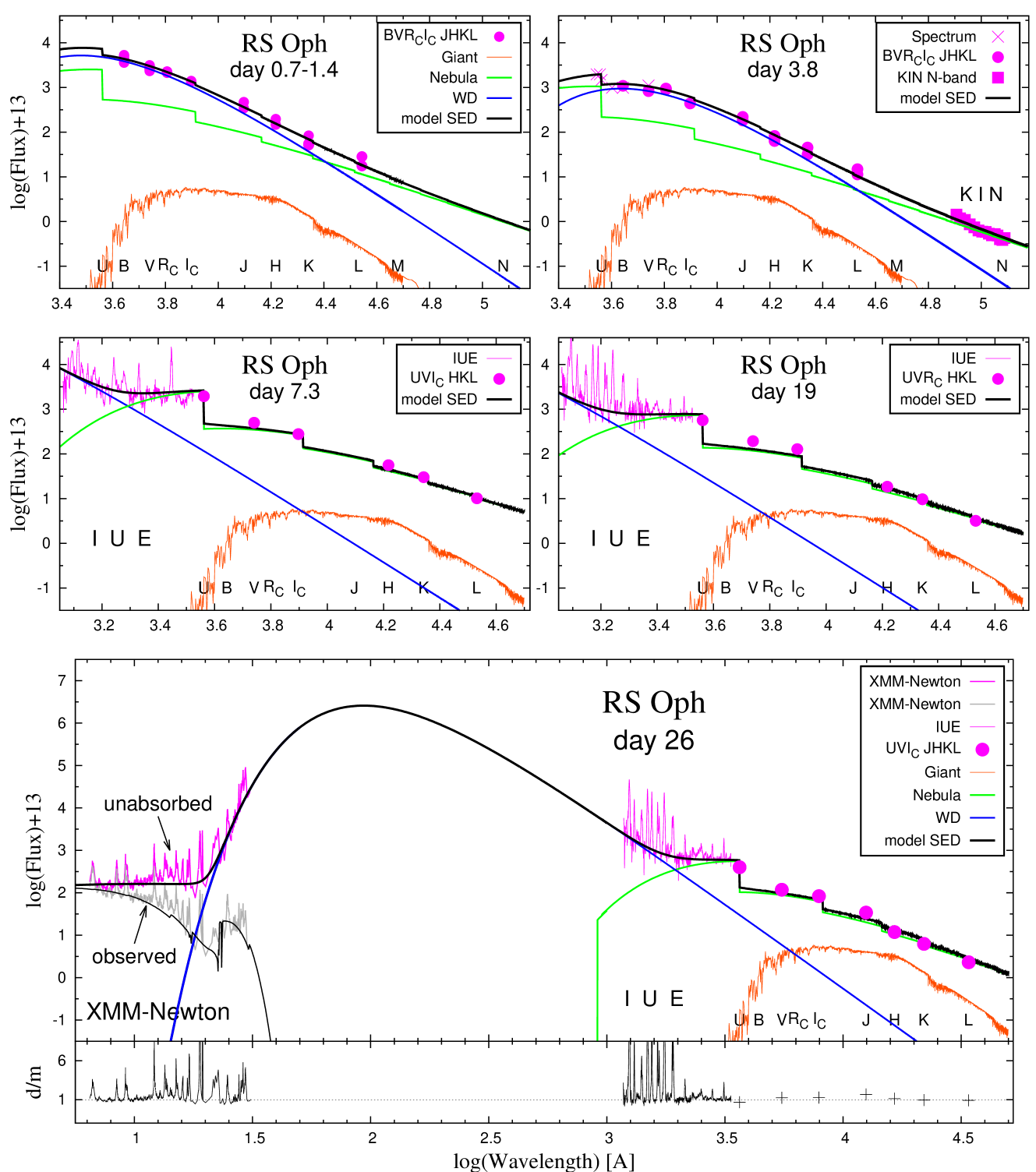
Figure 3: A comparison of the measured SED (in violet) and model SED (black solid line) of RS Oph from day 1 after its explosion to day 26. Data-to-model ratios (d/m) are plotted for the day-26 SED to judge the reliability of the fit. Models are described in Sect. 3 and their parameters given in Table 2. Fluxes are in units $\,\rm erg\,cm^{-2}\,s^{-1}\,\AA^{-1}$.

3.4 The first UV fluxes: Day 7.3 and beyond

The first observation covering the UV was made at day 7.3 after the outburst. It showed that the maximum of the SED shifted to higher energies. The observed steep slope of the far-UV continuum with increasing fluxes for $\lambda<$1600 Å suggested $T_{\rm h}\gtrsim 50000$ K. On the other hand, a flat horizontal profile of the continuum for $\lambda\gtrsim$2000 Å to the Balmer jump and its following gradual decrease to the IR domain suggested the presence of a strong nebular continuum produced by the thermal plasma. Therefore, subtracting the contribution from the giant, we can model the selected UV–near-IR fluxes with the function, $F(\lambda)=F_{\rm h}(\lambda)+F_{\rm n}(\lambda)$ (see Eq. (11) of Paper I).

However, observing only the Rayleigh-Jeans tail of the hot star radiation, which dominates a very short wavelength region of $\sim$1150–1600 Å, did not allow to determine unambiguously its temperature from modelling the SED. To the contrary, the nebular component dominates a significant part of the available spectrum including its maximum at the near-UV, which allowed to determine its parameters ($T_{\rm e}$ and $EM$) unambiguously, within uncertainties of the observed fluxes (to $\lesssim 10$ %). Assuming that the nebular emission represents a fraction of the hot star (i.e. the burning WD) radiation, re-processed via the ionization/recombination events, we can determine only a lower limit of its temperature, $T_{\rm h}^{\rm min}$, at which the flux of ionizing photons just balances the rate of recombinations giving rise to the observed $EM$ (see Apendix A).

Accordingly, in fitting the UV/near-IR continuum at day 7.3 to 19.5, I fixed the temperature of the ionizing source to $T_{\rm h}^{\rm min}$, which allowed to determine only limiting values of other depending parameters. For example, at day 7.3 the model SED gives $k_{\rm n}=7.8\times 10^{17}$ cm^-5 (i.e. $EM=2.4\times 10^{62}(d/1.6\,{\rm kpc})^{2}$ cm^-3) and $T_{\rm e}=17000$ K (i.e. $\alpha_{\rm B}({\rm H},T_{\rm e})=1.67\times 10^{-13}$ cm³ s^-1), which corresponds to $T_{\rm h}^{\rm min}=110000$ K for $F_{\rm h}$(1430 Å) = $3.6\times 10^{-10}$$\,\rm erg\,cm^{-2}\,s^{-1}\,\AA^{-1}$ (see Eq. (12)). Consequently, the luminosity of the burning WD, $L_{\rm h}>L(T_{\rm h}^{\rm min})=2.2\times 10^{39}$$\,\rm erg\,s^{-1}$, i.e. $>13\,L_{\rm Edd}$ (see Eqs. (9) and (13), Fig 5) and the effective radius of the ionizing source, $R_{\rm h}^{\rm eff}<2.1$ $R_{\odot}$.

The IUE observation at day 19.5 was the last one prior to the emergence of a supersoft X-ray component (see Fig. 1 of Ness et al., 2009). At this day, the nebular radiation was still very strong having the $EM=8.5\times 10^{61}(d/1.6\,{\rm kpc})^{2}$ cm^-3 and $T_{\rm e}=19500$ K. The far-UV continuum was estimated to $1.5\times 10^{-10}$$\,\rm erg\,cm^{-2}\,s^{-1}\,\AA^{-1}$ at $\lambda$ = 1280 Å, which yields $T_{\rm h}^{\rm min}=112000$ K, $R_{\rm h}^{\rm eff}<1.1$ $R_{\odot}$ and $L_{\rm h}>6.9\times 10^{38}$$\,\rm erg\,s^{-1}$, i.e. $>4\,L_{\rm Edd}$.

3.5 The first supersoft X-rays: Day 26

At day 26, it was the first possibility to model the SED of RS Oph with the supersoft X-ray emission (see Sect. 2.5). Fitting the significant part of the total spectrum, from the supersoft X-rays (here for $\lambda>20$ Å) to the IR domain, allowed to determine all 5 variables of the model SED unambiguously ($\theta_{\rm h}$, $T_{\rm h}$, $N_{\rm H}$, $k_{\rm n}$ and $T_{\rm e}$; see Eq. (11) and Sect. 4.2 of Paper I). The best model ($\chi^{2}_{\rm red}=2.8$ for 19 d.o.f.) corresponds to parameters of the stellar source $F_{\rm h}(\lambda)$: $N_{\rm H}=(7.4\pm 0.4)\times 10^{21}$ cm^-2, $T_{\rm h}=(310000\pm 10000)$ K and $\theta_{\rm h}=(8.4\pm 0.6)\times 10^{-12}$ (i.e. $R_{\rm h}^{\rm eff}=(0.6\pm 0.04)(d/1.6\,{\rm kpc})$ $R_{\odot}$), which yields $L_{\rm h}=(1.1\pm 0.22)\times 10^{40}(d/1.6\,{\rm kpc})^{2}$$\,\rm erg\,s^{-1}$. The nebular component, $F_{\rm n}(\lambda)$, is determined with $k_{\rm n}=(2.0\pm 0.2)\times 10^{17}$ cm^-5 (i.e. $EM=(6.2\pm 0.6)\times 10^{61}(d/1.6\,{\rm kpc})^{2}$ cm^-3) and $T_{\rm e}=(20000\pm 3000)$ K. The WD’s pseudophotosphere thus dominated both the supersoft X-ray and the far-UV, whereas the nebular component dominated the remainder of the spectrum for $\lambda\gtrsim 2000$ Å (Fig. 3).

Table 2: Physical parameters of the outbursting WD in RS Oph from day $\sim 1$ to day 26 (Sect. 3, Fig. 3).

Day	$N_{\rm H}$	$T_{\rm h}$	$\theta_{\rm h}$	$R_{\rm h}^{\rm eff}$	$\log(L_{\rm h}$)	$T_{\rm e}$	$EM$	$L_{\rm n}$	$\chi^{2}_{\rm red}$ / d.o.f.
	[$10^{21}$ cm-2]	[K]		[$R_{\odot}$]	[$\,\rm erg\,s^{-1}$]	[K]	[cm-3]	[$\,\rm erg\,s^{-1}$]
0.66–1.4	–	$9600\pm 300$	$(2.2\pm 0.2)\times 10^{-9}$	$156\pm 14$	$38.86\pm 0.11$	22000†	3.2$\times 10^{62}$	$2.6\times 10^{38}$	2.9 / 10
3.8	–	$6700\pm 200$	$(2.3\pm 0.2)\times 10^{-9}$	$163\pm 14$	$38.28\pm 0.10$	22000	1.3$\times 10^{62}$	$1.1\times 10^{38}$	2.8 / 31
7.3	–	$>110000^{\ddagger}$	$<2.9\times 10^{-11}$	$<2.1$	$>39.34$	17000	2.4$\times 10^{62}$	$2.1\times 10^{38}$	1.6 / 11
14.6	–	$>93000^{\ddagger}$	$<2.6\times 10^{-11}$	$<1.9$	$>38.96$	16000	9.8$\times 10^{61}$	$8.7\times 10^{37}$	2.6 / 12
19.5	–	$>112000^{\ddagger}$	$<1.6\times 10^{-11}$	$<1.1$	$>38.84$	19500	8.5$\times 10^{61}$	$7.2\times 10^{37}$	1.4 / 11
26.1	7.4$\pm 0.3$	$310000\pm 10000$	$(8.4\pm 0.6)\times 10^{-12}$	0.60$\pm 0.04$	$40.05\pm 0.08$	20000	6.2$\times 10^{61}$	$5.2\times 10^{37}$	2.8 / 20

^† fixed value, ^‡ = $T_{\rm h}^{\rm min}$ (Sect. 3.4, Appendix A).

The spectral range between $\sim 6$ and $\sim 19$ Å was dominated by a flat harder component. This part of the X-ray spectrum was compared with a function

$$F_{\rm E}=k_{\rm E}E^{-\alpha}e^{-E/\beta}e^{-\sigma_{\rm x}N_{\rm H}},$$ (2)

where the flux of photons $F_{\rm E}$ at the energy $E$ (keV) is in ’photons/s/cm²/keV’, $k_{\rm E}$ is a scaling factor and $\alpha$, $\beta$ are fitting parameters. Figure 3 shows a model for $k_{\rm E}=0.15$ photons/s/cm²/keV, $\alpha=2.8$, $\beta=5.5$ keV and $N_{\rm H}=7.4\times 10^{21}$ cm^-2. The absorbed flux of this harder (6.5–19.3 Å) component was $9.6\times 10^{-11}$$\,\rm erg\,cm^{-2}\,s^{-1}$, which corresponds to the unabsorbed value of $3.8\times 10^{-10}$$\,\rm erg\,cm^{-2}\,s^{-1}$. I note that the total (6.5–31.0 Å) absorbed flux of $1.3\times 10^{-10}$$\,\rm erg\,cm^{-2}\,s^{-1}$ is comparable with that obtained by Nelson et al. (2008). The origin of this component is probably connected with the optically thin, a few millions of kelvins hot, collisionally-ionized plasma (Bode et al., 2006), heated by shock waves in the highly-supersonic mass-outflow.

4 Discussion

4.1 Biconical ionization structure during the first 4 days

Multiwavelength modelling of the SED revealed the simultaneous presence of a warm stellar ($F_{\rm h}(\lambda)$) and nebular ($F_{\rm n}(\lambda)$) components of radiation in the spectrum of RS Oph during the first four days after its explosion. The stellar component is characterized with $T_{\rm h}=9600-6700$ K and $L_{\rm h}=7.2-1.9\times 10^{38}$$\,\rm erg\,s^{-1}$, which corresponds to production of $4.4\times 10^{45}-1.1\times 10^{42}$ photons per second that are capable of ionizing hydrogen. However, the nebular component is characterized with $\textsl{EM}\sim 2.3\times 10^{62}$ cm^-3, which corresponds to $\sim 3\times 10^{49}$ recombinations per second $(\alpha_{\rm B}({\rm H},22000\,K)=1.33\times 10^{-13})$, and thus cannot be generated by the observed stellar source of radiation ($L_{\rm ph}\lll\alpha_{\rm B}\textsl{EM}$; see Eq. (8)). This implies the presence of a hot ionizing source in the system, which is not seen directly by the outer observer. Such properties of radiative components were revealed in the spectrum of all symbiotic stars with a high orbital inclination during their outbursts. The corresponding spectrum was called a two-temperature-type (see Sect. 5.3.4 of Skopal, 2005). This puts constraints for the ionization and geometrical structure of the circumstellar matter surrounding the burning WD. According to Skopal (2005) the source of the warm stellar component can be ascribed to the WD’s pseudophotosphere that is represented by the outer flared rim of an optically thick disk-like formation around the hot star. The circumstellar material located within the remainder of the sphere is ionized, and thus converts a fraction of the hot star (here the burning WD) radiation into the strong nebular emission (see Fig. 4).

4.1.1 Nature of the ionized region

Ever since the very beginning of the nova explosion (day 1.16), very broad emission lines of hydrogen were observed in the optical spectrum (e.g. Banerjee et al., 2009). Skopal et al. (2008b) fitted the broad wings of H$\alpha$ from day 1.38 by the wind model of Skopal (2006), in which a fraction of the wind from the central star is blocked by a disk around the WD’s equator, and thus causes its bipolarity. The very high level of the continuum around the H$\alpha$ line of $2.5\times 10^{-10}$$\,\rm erg\,cm^{-2}\,s^{-1}\,\AA^{-1}$ (see Fig. 3, left top panel) yields its luminosity, $L_{\alpha}\sim 4900$ $L_{\odot}$ and the mass loss rate of a few $\times\,10^{-4}$ $M_{\odot}\,{\rm yr}^{-1}$ (Skopal et al., 2008b). Consequently, the H$\alpha$ luminosity was generated in a volume with the emission measure EM${}_{\alpha}=L_{\alpha}/\varepsilon_{\alpha}\sim 10^{62}(d/1.6\,{\rm kpc})^{2}$ cm^-3 for $\varepsilon_{\alpha}(20000\,K)=1.83\times 10^{-25}$ erg cm³ s^-1, which is consistent with that of the nebular continuum. As both the nebular continuum and the hydrogen emission lines originate in the same region, the HII zone, producing the strong nebular component of radiation in the SED, can be ascribed to the fast ionized wind from the outbursting WD.

In addition, the biconical structure and the nature of the ionized zone was also supported by the presence of satellite emission components located at $\pm(2400-2500)$ km s^-1 with respect to the main cores of hydrogen lines, measured from the very beginning of the outburst and being recognizable to day $\sim 30$ (Skopal et al., 2008b; Banerjee et al., 2009). These emission features can be interpreted as a result of highly collimated bipolar mass outflow. This was confirmed by the radio 43 GHz image from day 55 that showed directly highly collimated outflows produced by free-free emission from the thermal plasma (Sokoloski et al., 2008). The presence of bipolar jets requires the presence of the inner disk, throughout which sufficient amount of mass must be accreted to balance the outflow via the jets (e.g. Livio et al., 2003). Thus the presence of a large disk-like formation encompassing the burning WD could also be responsible for keeping the super-Eddington luminosity of the burning WD for a long time.

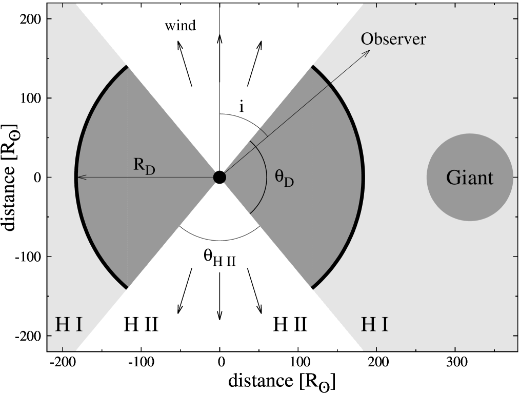
Figure 4: A sketch of the ionization structure of RS Oph during the first 4 days after its explosion as seen on a cut perpendicular to the orbital plane containing the burning WD (the black circle). The neutral (H I) zone is optically thick to the distance $R_{\rm D}$ from the WD, which represents the radius of the warm pseudophotosphere (heavy solid line). The ionized (H II) zone has the opening angle $\theta_{\rm HII}$. Dimensions in the figure are given by the model SED and the elements of the spectroscopic orbit according to Brandi et al. (2009).

4.1.2 Consequences of the bipolar structure

(i) The bolometric luminosity of the burning WD cannot be determined unambiguously during this period of the nova evolution. Only its lower limit can be estimated from the components of radiation determining the observed two-temperature-type of the spectrum. The disk-like shell around the WD converts a fraction of its radiation into the warm stellar component (here approximated by blackbody). Its luminosity at day $\sim 1$ was $7.3\times 10^{38}$$\,\rm erg\,s^{-1}$ (Table 2). Another fraction of the burning WD’s luminosity is reprocessed by ionization/recombination events into the nebular component. Its luminosity can be expressed as (see Eq. (8) in Paper I)

$$L_{\rm n}=\textsl{EM}\int_{\lambda>912}^{\infty}\varepsilon_{\lambda}(T_{\rm e}){\rm d}\lambda,$$ (3)

where the nebula is assumed to radiate under conditions of Case B. The EM(day $\sim 1)=3.2\times 10^{62}$ cm^-3 corresponds to $L_{\rm n}=2.6\times 10^{38}$$\,\rm erg\,s^{-1}$. This also represents a lower limit, because a fraction of ionizing photons is not detectable (they are not converted into the nebular photons, i.e. $L_{\rm ph}>\alpha_{\rm B}\textsl{EM}$, see Appendix A) and, in addition, the nebula can be partially optically thick (i.e. the measured EM is smaller than that originally created by ionizations). Thus the bolometric luminosity of the burning WD is

$$L_{\rm h}^{\rm bol}>L_{\rm h}+L_{\rm n}=9.9\times 10^{38}\,{\rm erg}\,{\rm s}^{-1}$$ (4)

at day $\sim 1$. Note that such adding of luminosities from different sources to the bolometric luminosity is possible only in the case of the two-temperature-type of the spectrum (i.e. the warm pseudophotosphere is far below the capability of giving rise to the observed nebular component of radiation).

(ii) According to the bipolar ionization structure of the burning WD, the vertical extension of the warm pseudophotosphere is limited by the orbital inclination to get hidden the ionizing source in direction of the observer. Its luminosity can be written as

$$S(R_{\rm D},\theta_{\rm D})\sigma T_{\rm eff}^{4}=4\pi(R_{\rm h}^{\rm eff})^{2}\sigma T_{\rm eff}^{4},$$ (5)

where the surface $S(R_{\rm D},\theta_{\rm D})$ of the pseudophotosphere is represented by a belt on a sphere with the radius $R_{\rm D}$, located around its equator and extended to the latitude $\pm\theta_{\rm D}/2$ (see Fig. 4). $R_{\rm h}^{\rm eff}$ is its effective radius (see Eq. (6) in Paper I). Then the radial extension of such the pseudophotosphere can be expressed as

$$R_{\rm D}=\frac{R_{\rm h}^{\rm eff}}{\sqrt{\sin(\theta_{\rm D}/2)}}.$$ (6)

For $R_{\rm h}^{\rm eff}\sim 160$ $R_{\odot}$ (Table 2) and the limiting case $\theta_{\rm D}/2=90^{\circ}-i$, where $i=50^{\circ}$, we get $R_{\rm D}=200$ $R_{\odot}$. Other possibilities, $40^{\circ}<\theta_{\rm D}/2<90^{\circ}$ yield $200>R_{\rm D}>160$ $R_{\odot}$.

4.1.3 Comparison with other measurements

At day 3.8 after the nova explosion, Barry et al. (2008b) used the KIN to find the structure of the circumstellar material around the star. They determined the angular size of the mid-infrared continuum emitting material to 4.0–6.2 mas, which corresponds to linear size of 6.4–9.9(d/1.6 kpc) AU. As the N-band region is dominated by the nebular emission (see Fig. 3), which is due to the fast ionized wind from the WD (see Sect. 4.1.1), its maximum extension (13 AU for the velocity of 3000 km s^-1 and 3.8 days) is consistent with that detected by the KIN. The measurements obtained by the KIN in the inner spatial regime showed evidence of enhanced neutral atomic hydrogen emission and atomic metals located near the WD. This could reflect the H I zone in the ionization structure inferred from the model SED (Fig. 4).

Monnier et al. (2006) measured the near-IR size of RS Oph using the IOTA and Keck interferometer at the same day. They found a significantly asymmetric emission with the characteristic size of FWHM$\sim 3$ mas. Observations for the following 60 days did not indicate any change, suggesting thus that the IR emission is due to the $b-f$ and $f-f$ transitions in thermal plasma rather than from a hot gas in the expanding shock as considered in current popular models. Also these results – the size and the nature of the IR emission – are consistent with the model SED here.

Using the AMBER/VLT interferometer, Chesneau et al. (2007) measured the extension of the milliarcsecond-scale emission in the K band continuum, in the Br${\gamma}$ and He I 2.06 $\mu$m lines at day 5.5. Observations showed that the emission from all investigated spectral regions is highly flattened with the ratio $b/a\sim 0.6$, having the same position angle and a typical Gaussian extension of $3.1\times 1.9$ mas for the continuum.

Thus, it is possible to conclude that the biconical ionization structure of the circumstellar matter around the WD in RS Oph, as inferred from multiwavelength modelling the SED, is supported by direct interferometric measurements using IOTA, Keck and AMBER/VLTI performed during a few days after the eruption.

4.2 Sudden transition of the SED maximum to the UV

The model SED for day 7.3 showed that the shift of the SED maximum from the optical to the far-UV (or even beyond) happened during a relatively short time of $<3.5$ days (see Fig. 3). A sudden decrease of the optical depth causing the shrinkage of the inflated WD from $\sim 160$ $R_{\odot}$ to less than 2.1 $R_{\odot}$ (Table 2) would require removal of a significant amount of dense, optically thick, material in the line of sight. The corresponding time of such the change should be proportional to the dynamical time scale of the inflated WD,

$$t_{\rm dyn}=(G\rho)^{-1/2},$$ (7)

where $\rho$ is the density of the matter giving rise to the gravitational force. So, for the WD mass of $1.3$ $M_{\odot}$, its effective radius 160 $R_{\odot}$ would collapse during $t_{\rm dyn}=67$ days, which is by a factor of $\sim 20$ larger than the time scale of the observed change in the effective radius. Therefore, a gradual shrinking of the WD pseudophotosphere due to the expansion of the outflowing material cannot be the cause of its sudden disappearance between day 3.8 and 7.3.

The sudden change in the SED can be a result of a change in the position of the ionization boundary with respect to the line of sight. If the opening angle of the H I zone $\theta_{\rm D}$ (see Fig. 4) shrinks so that $\theta_{\rm D}/2<90^{\circ}-i$, the burning WD will rise up the horizon represented by the H I/H II boundary. A shrinkage/enlargement of the $\theta_{\rm D}/\theta_{\rm HII}$ angle can be a result of a decreasing mass loss rate from the WD. Recently, Cariková & Skopal (2012) found that the ionization structure of the hot components in symbiotic binaries during outbursts is similar to that sketched in the figure 4 here (see their Figs. 1 and 6). In their model, the opening angle of the H II zone, $\theta_{\rm HII}$, is related to the mass loss rate from the WD as $\dot{M}_{\rm wind}^{-2}$. This implies that a relatively small decrease in the $\dot{M}_{\rm wind}$ can yield a large increase in the $\theta_{\rm HII}$ angle (see Fig. 1 of Cariková & Skopal, 2012). During the first days, when the $\dot{M}_{\rm wind}$ was at a maximum, $\theta_{\rm HII}/2<i$ (i.e. the hot WD was below the H I/H II boundary), because we observed the warm pseudophotosphere. A small decrease in $\dot{M}_{\rm wind}$ could lead to opening of the H II zone so that $\theta_{\rm HII}/2>i$, i.e. the burning WD raised up the H I/H II horizon and thus we could observe directly its hot $\lesssim 2.1$ $R_{\odot}$ photosphere at day 7.3. This could happen in a short time, because of a relatively low value of $i$. A transient increase of the EM at day 7.3 supports this view.

4.3 Long-lasting super-Eddington luminosity

Multiwavelength modelling the SED revealed that the luminosity of the WD was super-Eddington during the whole period of its nuclear burning (Table 2 here and Table 2 of the following paper).

Prior to the emergence of supersoft X-rays, only the lower limit of the WD’s luminosity could be determined. During the presence of the two-temperature-type of the spectrum (i.e. for the first 4 days), it was given by the integral of directly measured fluxes (or their model) scaled with the distance. The model SED at day $\sim 1$ and 3.8 corresponded to the luminosity of 6 and 2 $L_{\rm Edd}$, respectively, for $M_{\rm WD}=1.3$ $M_{\odot}$. However, its true value was higher, because both the warm shell and the nebula converted only a fraction of the WD radiation into direction of the observer (Sect. 4.1.2, Eq. (4), Fig. 4).

From day 7.3, measuring only the short Rayleigh-Jeans tail of the hot WD radiation, only the lower limit of its temperature and luminosity could be determined (see Appendix A). Using the emission measure from the model SED and the $F_{\rm h}(\lambda)$ flux from the far-UV spectrum, allowed to determine the minimum temperature of the WD photosphere, $T_{\rm h}^{\rm min}\sim 10^{5}$ K (Eq. (12), Table 2) and the minimum of its luminosity, $L(T_{\rm h}^{\rm min})=13-4\,L_{\rm Edd}$ (Eq. (9)), at which the burning WD is just capable of producing the observed EM during day 7.3 – 19.5. Note that the luminosity of the nebular component itself corresponds to 1.24 $L_{\rm Edd}$ at day 7.3 (Table 2).

The emergence of the first supersoft X-rays from the WD at day 26 allowed to determine its luminosity unambiguously to $L_{\rm h}=65\pm 12$ $L_{\rm Edd}$ (Sect. 3.5). Such a highly super-Eddington luminosity contradicts theoretical predictions, treating the nova event as a simple nuclear bomb explosion. According to Starrfield et al. (2008) the luminosity can exceed the Eddington limit only at the very beginning of the nova eruption with a rapid decline below it on a time-scale of hours.

However, the opposite cases were reported by some authors already during 70’s and 80’s decades of the last century. For example, Friedjung (1987) showed that the energy output of the nova FH Ser was well above the Eddington limit for about two months after its optical maximum. The super-Eddington state was theoretically investigated by Shaviv (2001), who considerred a reduction of the effective opacity due to the rise of a ‘porous layer’ above the convective zone of the burning WD (see Fig. 1 of Shaviv & Dotan, 2010). These conditions enlarges the Eddington luminosity well above its classical value, calculated for the Thomson scattering opacity. The super-Eddington state also accelerates a thick continuum driven wind at high rates. The mass loss through the wind at a high rate of a few $\times\,10^{-4}-10^{-5}$ $M_{\odot}\,{\rm yr}^{-1}$ during the hydrogen burning period of RS Oph (Skopal et al., 2008b) is consistent with that suggested for the super-Eddington state (Eq. (30) of Shaviv, 2001, for $v_{\rm s}$ = 20 - 50 km s^-1). In addition, the presence of the bipolar jets for the first 30 days (Skopal et al., 2008b; Banerjee et al., 2009), which suggests accretion throughout the disk at a high rate, also supports the super-Eddington state. For example, accretion at $\dot{m}\sim 2\times 10^{-5}$ $M_{\odot}\,{\rm yr}^{-1}$ can release its binding energy $GM_{\rm WD}\dot{m}/R_{\rm WD}\sim 10^{39}$$\,\rm erg\,s^{-1}$, and thus help to sustain the high luminosity of the accretor for a long time.

Finally, it is important to note that the high energy output released during the outburst of RS Oph, as given by the global model SED of this paper, is more than a factor of 10 larger than that so far derived. This requires a very high accretion rate, which is far above that can be obtained from a spherical wind mass loss of the giant (e.g. Schaefer, 2009). Considering that the primary source of the material powering the outburst is the wind from the giant, then a different, more efficient mechanism of the mass transfer onto the WD must be in the effect. This could be realized by the so-called wind Roche-lobe overflow (WRLOF), which can occur when the wind acceleration zone is stretched out to the Roche lobe of the giant (e.g. Mohamed & Podsiadlowski, 2007; Abate et al., 2013). In this case the wind of the giant is focused towards the orbital plane and in particular towards the WD. The accretion rate predicted in the WRLOF regime can be 100 times larger than the rate expected from standard Bondi-Hoyle accretion (see Mohamed & Podsiadlowski, 2007).

More detailed discussion on the accretion mechanism is presented in the following paper, RS Ophiuchi: The supersoft X-ray phase and beyond, where other critical parameters are determined from the model SEDs during the SSS phase and following quiescence.

5 Summary

In this paper I applied the method of multiwavelength modelling the SED (see Paper I) to the recurrent symbiotic nova RS Oph from its explosion to the SSS phase (to day 26). The model SEDs revealed the presence of a strong stellar as well as nebular component of radiation in the spectrum. The contribution from the cool giant was negligible with respect to these components (Sect. 3, Fig. 3, Table 2). The main results can be summarized as follows.

1. The radiation from the giant corresponds to its effective temperature $T_{\rm eff}=3800-4000$ K, the radius, $R_{\rm g}=(61-55)\,(d/1.6\,{\rm kpc})$ $R_{\odot}$ and the luminosity, $L_{\rm g}=(690\pm 95)\,(d/1.6\,{\rm kpc})^{2}$ $L_{\odot}$. The giant underfills deeply its Roche lobe for d = 1.6 kpc (Sect. 3.1).

2. During the first 4 days after the explosion, the model SED identified a biconical ionization and geometrical structure of the nova. The $\sim 8200$ K warm pseudophotosphere was represented by a belt on a sphere with the radius of 160–200 $R_{\odot}$, located around the WD’s equator and extended to the latitude $>40^{\circ}$. The remaining space around the WD’s poles was ionized, producing a strong nebular emission ($\textsl{EM}\sim 2.3\times 10^{62}$ cm^-3) via the fast ionized wind from the WD (see Fig. 4, Sect. 4.1).

3. The luminosity of the burning WD was super-Eddington for the whole investigated period, although it was possible to determine only its lower limit prior to the emergence of the supersoft X-ray radiation (Sect. 4.3, Table 2).

   During the first 4 days, the luminosity $L_{\rm h}>2-6\,L_{\rm Edd}$ for $M_{\rm WD}=1.3$ $M_{\odot}$. Here the lower limit is given by the fit of the model SED to the total measured spectrum, because both the neutral and the ionized region convert only a fraction of the WD’s radiation into direction of the observer (Sect. 4.1.2).

   From day 7.3, the two-temperature-type of the spectrum suddenly disappeared, because the H II zone opened so that we could observe directly the hot WD (Sect. 4.2). In this case lower limits of the WD’s temperature and luminosity were determined from the condition that the corresponding flux of ionizing photons was just capable of producing the observed EM (Sect. 4.3, Eq. (8)). Here the model SEDs suggested $L_{\rm h}>4-13\,L_{\rm Edd}$.

   At day 26, the first detection of the supersoft X-ray fluxes allowed to determine the WD’s luminosity unambiguously to $L_{\rm h}=65\pm 12$ $L_{\rm Edd}$ (Sect. 3.5, Fig. 3).

4. The long-lasting super-Eddington luminosity and the mass loss at a very high rate are consistent with theoretical considerations treating the super-Eddington state as a result of a reduction the effective opacity of the WD atmosphere. However, the appearance of highly super-Eddington luminosity just at the beginning of the SSS phase (day 26) is enigmatic, unless this could also be connected with a relevant reduction of the effective opacity. The presence of collimated jets during the burning phase suggests an accretion throughout a disk during this period, which can help to balance the high energy output for a long time. This means that the disk was not destroyed by the eruption.

5. The high energy output released during the outburst of RS Oph requires a very high accretion rate, which could be realized in the WRLOF regime.

Further analysis and discussion on the accretion mechanism is found in the following paper, RS Ophiuchi: The supersoft X-ray phase and beyond.

Appendix A A minimum $T_{\rm h}$ and $L_{\rm h}$ of the ionizing source from the observed EM

Here we determine the lower limit of the temperature and luminosity of the ionizing source, at which the corresponding flux of ionizing photons gives rise to the observed $EM$. The method is based on the fact that the nebular component of radiation represents a fraction of the hot stellar radiation reprocessed via the ionization/recombination events. The result of this process depends on the number of ionizing photons produced by the hot star and the number of particles on their path that are subject to ionization. In the limiting case, when all the ionizing photons are converted into the diffuse radiation, we can approximate the equilibrium condition between the flux of ionizing photons $L_{\rm ph}$ and the rate of recombinations in the nebula as

$$L_{\rm ph}({\rm H})\,=\,\alpha_{\rm B}({\rm H},T_{\rm e})\,\textsl{EM},$$ (8)

where $\alpha_{\rm B}({\rm H},T_{\rm e})$ (cm³ s^-1) is the recombination coefficient to all but the ground state of hydrogen (i.e. for Case $B$). This equation is valid for the hydrogen plasma, heated by photoionizations, and characterized with a constant $T_{\rm e}$ and particle concentration. Thus, the $EM$ constrains a minimum luminosity of $L_{\rm ph}$ photons, which is a function of $T_{\rm h}$ and $L_{\rm h}$ of the hot ionizing source. Using the expression for the $L_{\rm ph}$ function (see Eq. (11) of Skopal, 2001), the luminosity of the ionizing source, which is capable of producing the observed EM, can be written as

$$L(T_{\rm h})=\alpha_{\rm B}({\rm H},T_{\rm e})\,\textsl{EM}\frac{\sigma T_{\rm h}^{4}}{f(T_{\rm h})},$$ (9)

where the function

$$f(T_{\rm h})=\frac{\pi}{hc}\int^{\rm 912\AA}_{0}\!\!\!\lambda\,B_{\lambda}(T_{\rm h})\,\rm d\lambda.$$ (10)

Examples of the $L(T_{\rm h})$ function parametrized with different values of EM are plotted in Fig. 5. Its minimum corresponds to the temperature, at which the source produces maximum flux of ionizing photons (for hydrogen it is 73000 K). For higher/lower $T_{\rm h}$ it increases, because of decreasing production of the ionizing photons for a given $L_{\rm h}$.

For $T_{\rm h}\gtrsim 50000$ K we can observe only the Jeans tail of the hot source radiation in the ultraviolet. This implies that a small part of the far-UV fluxes increasing to higher energies can be compared with any blackbody radiation from this range of temperatures. If we have available an appropriate spectrum, a $Zanstra$-tepmerature can be adopted. Here, according to Eq. (8), we determine a minimum temperature $T_{\rm h}^{\rm min}$ of the ionizing source, at which the blackbody radiation, scaled to the far-UV fluxes, is just capable of producing the observed EM. According to Skopal (2005) we can get $T_{\rm h}^{\rm min}$ by solving equation

$$\frac{k_{\rm n}}{k_{\rm h}(T_{\rm h})}\alpha_{\rm B}({\rm H},T_{\rm e})-f(T_{\rm h})=0,$$ (11)

where $k_{\rm n}$ and $T_{\rm e}$ are fitting parameters (see Sect. 2.4 of Paper I) and $k_{\rm h}(=\theta_{\rm h}^{2})$ scales the blackbody flux emitted by the ionizing source to its observed flux $F_{\rm h}(\lambda)$. Then, Eq. (11) can be expressed as

$$\frac{k_{\rm n}}{F_{\rm h}(\lambda)}\alpha_{\rm B}({\rm H},T_{\rm e})\pi B_{\lambda}(T_{\rm h})-f(T_{\rm h})=0,$$ (12)

where $F_{\rm h}(\lambda)$ is selected at a wavelength $\lambda$, at which the ionizing source dominates the spectrum (usually in the far-UV). Its solution for the input quantities of $k_{\rm n}$, $F_{\rm h}(\lambda)$, $\lambda$ and $\alpha_{\rm B}({\rm H},T_{\rm e})$ provides $T_{\rm h}\equiv T_{\rm h}^{\rm min}$.

According to Eq. (9), this temperature determines the minimum luminosity $L(T_{\rm h}^{\rm min})$, at which the ionizing source is just capable of producing the observed EM. In the real case, a fraction of the ionizing photons can escape the star without being converted into the nebular radiation. Also the measured EM represents a lower limit of what was originally created by ionizations, because we observe only the optically thin part of the nebula. Under these circumstances the luminosity of the $L_{\rm ph}$ photons, originally emitted by the source, is larger than that given by the equilibrium condition (8), i.e. $L_{\rm ph}>\alpha_{\rm B}({\rm H})\,$EM, which according to Eq. (9) implies

$$L_{\rm h}>L(T_{\rm h}^{\rm min})$$ (13)

even for $T_{\rm h}=T_{\rm h}^{\rm min}$. Considering that $T_{\rm h}$ can be $>T_{\rm h}^{\rm min}$ and the nebula during outbursts is ionization bounded, it is probable that $L_{\rm h}\gg L(T_{\rm h}^{\rm min})$.

Figure 5: The lower limit of the WD luminosity as a function of its temperature scaled with EM (Eq. (9)) derived from the model SED on day 7.3, 14.6 and 19.5. The thick arrows start at $T_{\rm h}^{\rm min}$ (Table 2).

References

- Abate et al. (2013) Abate, C., Pols, O. R., Izzard, R. G., Mohamed, S. S., de Mink, S. E.: 2013, A&A, 552, A26
- Anupama (2008) Anupama, G. C.: 2008 in ASP Conf. Ser. 401, RS Ophiuchi (2006) and the Recurent Nova Phenomenon, eds. A. Evans, M. F. Bode, T. J. O’Brien and M. J. Darnley, (San Francisco: ASP), 251
- Banerjee et al. (2009) Banerjee, D. P. K., Das, R. K., Ashok, N. M.: 2009, MNRAS, 399, 357
- Barry et al. (2008a) Barry, R. K., Mukai, K., Sokoloski, J. L., Danchi, W. C., Hachisu, I., Evans, A., Gehrz, R., Mikolajewska, J.: 2008a, in Evans A., Bode M. F., O’Brien T. J., Darnley M. J., eds, ASP Conf. Ser. 401, RS Ophiuchi (2006) and the Recurrent Nova Phenomenon. ASP, San Francisco, p. 52
- Barry et al. (2008b) Barry, R. K., W. C. Danchi, W. A., Traub, et al.: 2008b, ApJ, 677, 1253
- Bode (1987) Bode, M. F.: 1987, in Bode M. F., ed, RS Ophiuchi (1985) and the Recurrent Nova Phenomenon. VNU Science Press, Utrecht, p. 241
- Bode et al. (2006) Bode, M. F., O’Brien, T. J., Osborne, J. P., Page, K. L., Senziani, F., Skinner, G. K., Starfield, S., Ness, J.-U.: 2006, ApJ, 652, 629
- Bode et al. (2007) Bode, M. F., Harman, D. J., O’Brien, T. J., et al.: 2007, ApJ, 665, L63
- Brandi et al. (2009) Brandi, E., Quiroga, C., Mikolajewska, J., Ferrer, O. E., García, L. G.: 2009, A&A, 497, 815
- Cariková & Skopal (2012) Cariková, Z., & Skopal, A.: 2012, A&A, 548, A21
- Chesneau et al. (2007) Chesneau, O., Nardetto, N., Millour, F., et al.: 2007, A&A, 464, 119
- Diplas & Savage (1994) Diplas, A., Savage, B. D.: 1994, ApJ, 427, 274
- Drake et al. (2009) Drake, J. J., Laming, J. M., Ness, J.-U., et al.: 2009, ApJ, 691, 418
- Dumm & Schild (1998) Dumm, T., Schild, H.: 1998, New Astron., 3, 137
- Evans et al. (1988) Evans, A., Callus, C. M., Albinson, J. S., Whitelock, W. A., Glass, I. S., Carter, B., Roberts, G.: 1988, MNRAS, 234, 755
- Evans et al. (2007) Evans, A., Woodward, C. E., Helton, L. A., Gehrz, R. D., Lynch, D. K., Rudy, R. J., Russell, R. W., Kerr, T.: 2007, ApJ, 663, L29
- Fekel et al. (2000) Fekel, F. C., Joyce, R. R., Hinkle, K. H., Skrutskie, M.: 2000, AJ, 119, 1375
- Friedjung (1987) Friedjung, M.: 1987, A&A, 179, 164
- Hauschildt et al. (1999) Hauschildt, P. H., Allard, F., Ferguson, J., Baron, E., Alexander, D. R.: 1999, ApJ, 525, 871
- Hjellming et al. (1986) Hjellming, R. M., van Gorkom, J. H., Seaquist, R. E., Taylor, A. R., Padin, S., Davis, R. J., Bode, M. F.: 1986, ApJ, 305, L71
- Iijima (2009) Iijima, T.: 2009, A&A, 505, 287
- Lane et al. (2007) Lane, B. F., Sokoloski, J. L., Barry, R. K., et al.: 2007, ApJ, 658, 520
- Livio et al. (2003) Livio, M., Pringle, J. E., King, A. R.: 2003, ApJ, 593, 184
- Luna et al (2009) Luna, G. Luna, G. J. M., Montez, R., Sokoloski, J. L., Mukai, K., Kastner, J. H.: 2009, ApJ, 707, 1168
- Mohamed & Podsiadlowski (2007) Mohamed, S., Podsiadlowski, P.: 2007, in 15th European Workshop on White Dwarfs, eds. R. Napiwotzki, & M. R. Burleigh, ASP Conf. Ser., 372, 397
- Monnier et al. (2006) Monnier, J. D., Barry, R. K., Traub, W. A., et al.: 2006, Apj, 647, L127
- Mürset & Schmid (1999) Mürset, U., Schmid, H. M.: 1999, A&AS, 137, 473
- Narumi et al. (2006) Narumi, H., Hirosawa, K., Kanai, K., et al.: 2006, IAU Circ., 8671
- Nelson et al. (2008) Nelson, T., Orio, M., Cassinelli, J. P., Leibowitz, E., Mucciarelli, P.: 2008, ApJ, 673, 1067
- Ness et al. (2007) Ness, J.-U., Starrfield, S., Page, K. L., Osborne, J. P., Beardmore, A. P., Drake, J. J.: 2007a, PThPS, 169, 187
- Ness et al. (2009) Ness, J.-U., Drake, J. J., Starrfield, S., et al.: 2009, AJ, 137, 3414
- O’Brien et al. (2006) O’Brien, T., Bode, M. F., Porcas, R. W., Muxlow, T. W. B., Eyres, S. P. S., Beswick, R. J., Garrington, S. T., Davis, R. J., Evans, A.: 2006, Nature, 442, 279
- Osborne et al. (2011) Osborne, J. P., Page, K. L., Beardmore, A. P., et al.: 2011, ApJ, 727:124 (10pp)
- Pavlenko et al. (2008) Pavlenko, Ya. V., Evans, A., Kerr, T., et al.: 2008, A&A, 485, 541
- Rosino (1987) Rosino, L.: 1987, in Bode M. F., ed, RS Ophiuchi (1985) and the Recurrent Nova Phenomenon. VNU Science Press, Utrecht, p. 1
- Rupen et al. (2008) Rupen, M. P., Mioduszewski, A. J., Sokoloski, J. L.: 2008, ApJ, 688, 559
- Rushton et al. (2010) Rushton, M. T., Kaminsky, B., Lynch, D. K., et al.: 2010, MNRAS, 401, 99
- Schaefer (2009) Schaefer, B. E.: 2009, ApJ, 697, 721
- Shaviv (2001) Shaviv, N. J.: 2001, MNRAS, 326, 126
- Shaviv & Dotan (2010) Shaviv, N. J., Dotan, C.: 2010, Mem. S.A.It., 81 350
- Skopal (2001) Skopal, A.: 2001, A&A, 366, 157
- Skopal (2005) Skopal, A.: 2005, A&A, 440, 995
- Skopal (2006) Skopal, A.: 2006: A&A, 457, 1003
- Skopal (2007) Skopal, A.: 2007, New Astron., 12, 597
- Skopal (2014) Skopal, A.: 2014, New Astron., (in press, Paper I)
- Skopal et al. (2008a) Skopal, A., Vaňko, M., Komžík, R., Chochol, D.: 2008a, in Evans, A., Bode, M. F., O’Brien, T. J., Darnley, M. J., eds, ASP Conf. Ser. 401, RS Ophiuchi (2006) and the Recurrent Nova Phenomenon. ASP, San Francisco, p. 101
- Skopal et al. (2008b) Skopal, A., Pribulla, T., Buil, Ch., Vittone, A., Errico, L.: 2008b, in Evans, A., Bode, M. F., O’Brien, T. J., Darnley, M. J., eds, ASP Conf. Ser. 401, RS Ophiuchi (2006) and the Recurrent Nova Phenomenon. ASP, San Francisco, p. 227
- Snijders (1987) Snijders, M. A. J.: 1987, in in Bode M. F., ed, RS Ophiuchi (1985) and the Recurrent Nova Phenomenon. VNU Science Press, Utrecht, p. 51
- Sokoloski et al. (2006) Sokoloski, J. L., Luna, G. J. M., Mukai, K., Kenyon, S. J.: 2006, Nature, 442, 276
- Sokoloski et al. (2008) Sokoloski, J. L., Rupen, M. P., Mioduszewski, A. J.: 2008, ApJ, 685, L137
- Sostero & Guido (2006) Sostero, G., Guido, E.: 2006, IAU Circ. No. 8673
- Starrfield et al. (2008) Starrfield, S., Iliadis, Ch., Hix, W. R.: 2008, in M. F. Bode, & A. Evans, eds., Classical Novae. CUP, Cambridge, p. 77
- Taylor et al. (1989) Taylor, A. R., Davis, R. J., Porcas, R. W., Bode, M. F.: 1989, MNRAS, 237, 81
- van Belle et al. (1999) van Belle, G. T., Lane, B. F., Thompson, R. R., Boden, A. F., Colavita, M. M., Dumont, P. J., Mobley, D. W., Palmer, D., et al.: 1999, AJ, 117, 521
- West (2006) West, J. D.: 2006, IAU Circ. No. 8683
- Wilms et al. (2000) Wilms, J., Allen, A., McCray, R.: 2000, ApJ, 542, 914