Dragging of inertial frames inside the rotating neutron stars

Abstract

We derive the exact frame-dragging rate inside rotating neutron stars. This formula is applied to show that the frame-dragging rate monotonically decreases from the centre to the surface of the neutron star along the pole. In case of frame-dragging rate along the equatorial distance, it decreases initially away from the centre, becomes negligibly small well before the surface of the neutron star, rises again and finally approaches to a small value at the surface. The appearance of local maximum and minimum in this case is the result of the dependence of frame-dragging frequency on the distance and angle. Moving from the equator to the pole, it is observed that this local maximum and minimum in the frame-dragging rate along the equator disappears after crossing a critical angle. It is also noted that the positions of local maximum and minimum of the frame-dragging rate along the equator depend on the rotation frequency and central energy density of a particular pulsar.

1 Introduction

Compact astrophysical objects such as neutron stars and black holes are the laboratories for the study of Einstein’s general relativity in strong gravitational fields. The frame-dragging is one such important general relativistic effect as demonstrated by Lense and Thirring Lense & Thirring (1918). A stationary spacetime with angular momentum shows an effect by which the locally inertial frames are dragged along the rotating spacetime. This makes any test gyroscope in such spacetime precess with a certain frequency called the frame-dragging frequency or the Lense-Thirring (LT) precession frequency $(\Omega_{LT})$. The Lense-Thirring frequency is proportional to the angular momentum and compactness of the rotating astrophysical compact object. This effect for a test gyroscope had been calculated and was shown to fall with the inverse cube of the distance of the test gyroscope from the source and vanishes at large enough distances where the curvature effects are small. The precession frequency is thus expected to be larger near the surface of a neutron star and in its interior, rather than at large distance from the star.

The precise mass measurement of PSR J0348+0432 confirmed the existence of a massive neutron star ( $>2M_{\odot}$) (Antoniadis et al., 2013). It is also known that some of them are observed to possess very high angular velocities. Hence the spacetime curvature would be much higher in the surroundings of those massive neutron stars and the frame dragging effect also becomes very significant in the strong gravitational fields of those rotating neutron stars. It should be noted that the inertial frames are dragged not only outside but also inside the rotating neutron stars.

The theoretical prescription to determine the rate of the frame-dragging precession inside the rotating neutron star was first given by Hartle Hartle (1967). In this formalism, one can estimate the frame-dragging precession rate inside a slowly rotating ($\Omega R<<c$, where $R$ is the radius of the pulsar, $c$ is the speed of the light in vacuum) neutron star. The final expression of frame-dragging precession rate depends solely on $r$, the distance from the centre of the star, due to the slow rotation approximation, in Hartle’s formalism. It was observed that the frame-dragging frequency was higher at the centre of the star than the frame dragging frequency at the surface. The maximum frame dragging frequency at the centre $(r=0)$ would never exceed the frequency of the rotating neutron star. The frame-dragging effect was applied to various astrophysical problems using Hartle’s formalism. Hartle studied this effect on the equilibrium structures of rotating neutron stars (Hartle, 1968). The impact of frame dragging on the Kepler frequency was investigated by Glendenning and Weber (Glendenning & Weber, 1994). It was also demonstrated how this effect might influence the moment of inertia of a rotating neutron star (Weber, 1999). Furthermore, Morsink and Stella studied the role of frame dragging in explaining the Quasi Periodic Oscillations of accreting neutron stars (Morsink & Stella, 1999). Morsink and Stella estimated the precession frequency $\nu_{p}$ of the disk’s orbital plane about the star’s axis of symmetry as the difference between the frequency of oscillations of the particle along the longitude and latitude $(2\pi\nu_{p}=d\phi/dt-d\theta/dt)$ observed at infinity. This expression contains the total precession frequency of the disk’s orbital plane due to the Lense-Thirring (LT) effect as well as the star’s oblateness. Their calculation introduced zero angular momentum observer (ZAMO) and the precession frequency $\nu_{p}$ was observed at infinity. It was found that the LT frequency was proportional to the ZAMO frequency on the equatorial plane in the slow rotation limit. This is similar to the Hartle’s formalism(Hartle, 1967) where the angular velocity $(d\phi/dt)$ acquired by an observer who falls freely from infinity to the point $(r,\theta)$, is taken as the rate of rotation of the inertial frame at that point relative to the distant stars.

In this present manuscript we derive the exact Lense-Thirring precession frequency $(\Omega_{LT})$ which is measured by a Copernican observer of a gyroscope such as the Gravity Probe B satellite in a realistic orbitHartle (2009). In this case, $\Omega_{LT}$ would not only be the function of $\omega$ but a complicated function of other metric components also even in the slow rotation limit.

We should note that inside the rapidly rotating stars, one should not a priori expect the similar variation of the precession rates along the equatorial and polar plane. Thus the frame-dragging frequency should depend also on the colatitude ($\theta$) of the position of the test gyroscope. This did not arise in the formalism of Hartle due to the slow-rotation limit. We also note that the LT precession must depend on both the radial distance ($r$) and the colatitude ($\theta$) (see Eq.(14.34) of  Hartle (2009)) in very weak gravitational fields (far away from the surface of the rotating object).

The exact Lense-Thirring precession rate in strongly curved stationary spacetime had been discussed in detail by Chakraborty and Majumdar Chakraborty & Majumdar (2014). Later, Chakraborty and Pradhan Chakraborty & Pradhan (2013) applied this formulation in various stationary and axisymmetric spacetimes. Our main motivation of this paper is to compute the exact LT precession rate inside the rotating neutron star. In this article we avoid all types of approximations and assumptions to obtain the exact LT precession rate inside the rotating neutron stars.

The paper is organized as follows. In section 2 we present the basic equations of frame-dragging effect inside the rotating neutron stars. The numerical method, which has been adopted in the whole paper, is discussed in section 3. We discuss our results in section 4. Finally we conclude in section 5 with a summary.

2 Basic equations of frame-dragging effect inside the rotating neutron stars

The rotating equilibrium models considered in this paper are stationary and axisymmetric. Thus we can write the metric inside the rotating neutron star as the following Komatsu-Eriguchi-Hachisu (KEH) Komatsu et. al. (1989) form:

$$ds^{2}=-e^{\gamma+\sigma}dt^{2}+e^{2\alpha}(dr^{2}+r^{2}d\theta^{2})+e^{\gamma-\sigma}r^{2}\sin^{2}\theta(d\phi-\omega dt)^{2}$$ (1)

where $\gamma,\,\sigma,\,\alpha,\,\omega$ are the functions of $r$ and $\theta$ only. In the whole paper we have used the geometrized unit ($G=c=1$). We assume that the matter source is a perfect fluid with a stress-energy tensor given by

$$T^{\mu\nu}=(\rho_{0}+\rho_{i}+P)u^{\mu}u^{\nu}+Pg^{\mu\nu}$$ (2)

where $\rho_{0}$ is the rest energy density, $\rho_{i}$ is the internal energy density, $P$ is the pressure and $u^{\mu}$ is the matter four velocity. We are further assuming that there is no meridional circulation of the matter so that the four-velocity $u^{\mu}$ is simply a linear combination of time and angular Killing vectors. Now, we have to calculate the frame-dragging rate based on the above metric and this will gives us the exact frame-dragging rate inside a rotating neutron star.

We know that the vector field corresponding to the LT precession co-vector can be expressed as

$$\Omega_{LT}=\frac{1}{2}\frac{\epsilon_{ijl}}{\sqrt{-g}}\left[g_{0i,j}\left(\partial_{l}-\frac{g_{0l}}{g_{00}}\partial_{0}\right)-\frac{g_{0i}}{g_{00}}g_{00,j}\partial_{l}\right]$$ (3)

For the axisymmetric spacetime, the only non-vanishing component is $g_{0i}=g_{0\phi}$, $i=\phi$ and $j,l=r,\theta$; substituting these in Eq. (3), the LT precession frequency vector is obtained as:

$$\Omega_{LT}=\frac{1}{2\sqrt{-g}}\left[\left(g_{0\phi,r}-\frac{g_{0\phi}}{g_{00}}g_{00,r}\right)\partial_{\theta}-\left(g_{0\phi,\theta}-\frac{g_{0\phi}}{g_{00}}g_{00,\theta}\right)\partial_{r}\right]$$ (4)

As the above expression has been expressed in the co-ordinate basis we have to convert it into the orthonormal basis. Thus, in the orthonormal basis, with our choice of polar co-ordinates, $\Omega_{LT}$ can be written asChakraborty & Majumdar (2014)

$$\vec{\Omega}_{LT}=\frac{1}{2\sqrt{-g}}\left[\sqrt{g_{rr}}\left(g_{0\phi,\theta}-\frac{g_{0\phi}}{g_{00}}g_{00,\theta}\right)\hat{r}+\sqrt{g_{\theta\theta}}\left(g_{0\phi,r}-\frac{g_{0\phi}}{g_{00}}g_{00,r}\right)\hat{\theta}\right]$$ (5)

where $\hat{\theta}$ is the unit vector along the direction $\theta$ and $\hat{r}$ is the unit vector along the direction $r$. We note that the above formulation is valid only in the timelike spacetimes, not in the lightlike or spacelike regions.

Now, we can apply the above Eq.(5) to determine the exact frame-dragging rate inside the rotating neutron star of which the metric could be determined from the line-element(1). The various metric components can be read off from the metric. Likewise,

$$\sqrt{-g}=r^{2}e^{2\alpha+\gamma}\sin\theta$$ (6)

In orthonormal coordinate basis, the exact Lense-Thirring precession rate inside the rotating neutron star is:

$$\vec{\Omega}_{LT}=\frac{e^{-(\alpha+\sigma)}}{2(\omega^{2}r^{2}\sin^{2}\theta-e^{2\sigma})}.$$

$$\left[\sin\theta[r^{3}\omega^{2}\omega_{,r}\sin^{2}\theta+e^{2\sigma}(2\omega+r\omega,_{r}-2\omega r\sigma,_{r})]\hat{\theta}+[r^{2}\omega^{2}\omega_{,\theta}\sin^{3}\theta+e^{2\sigma}(2\omega\cos\theta+\omega_{,\theta}\sin\theta-2\omega\sigma_{,\theta}\sin\theta)]\hat{r}\right]$$

and the modulus of the above LT precession rate is

$$\Omega_{LT}=|\vec{\Omega}_{LT}(r,\theta)|=\frac{e^{-(\alpha+\sigma)}}{2(\omega^{2}r^{2}\sin^{2}\theta-e^{2\sigma})}.$$

$$\left[\sin^{2}\theta[r^{3}\omega^{2}\omega_{,r}\sin^{2}\theta+e^{2\sigma}(2\omega+r\omega,_{r}-2\omega r\sigma,_{r})]^{2}+[r^{2}\omega^{2}\omega_{,\theta}\sin^{3}\theta+e^{2\sigma}(2\omega\cos\theta+\omega_{,\theta}\sin\theta-2\omega\sigma_{,\theta}\sin\theta)]^{2}\right]^{\frac{1}{2}}$$

As a vector quantity the expression of $\vec{\Omega}_{LT}$ (Eq.2) depends on the coordinate frame (i.e. polar coordinates $(r,\theta)$ which is used here) but the modulus of $\vec{\Omega}_{LT}$ or $|\vec{\Omega}_{LT}|$ (Eq.2) must be coordinate frame independent. Here, we use only the modulus of $\Omega_{LT}$ in the rest of our manuscript.

To calculate the frame-dragging precession frequency at the centre of the neutron star we substitute $r=0$ in Eq. (2) and we obtain

$$\Omega_{LT}|_{r=0}=\left[\frac{{e^{-(\alpha+\sigma)}}}{2}\left[4\omega^{2}+(\omega_{,\theta}-2\omega\sigma_{,\theta})^{2}\sin^{2}\theta+4\omega\cos\theta\sin\theta(\omega_{,\theta}-2\omega\sigma_{,\theta})\right]^{\frac{1}{2}}\right]_{|{r=0}}$$ (9)

solving numerically $\omega_{,\theta}$ and $\sigma_{,\theta}$ at the centre we get the value zero for both of them. Thus, we obtain the frame-dragging precession rate

$$\Omega_{LT}|_{r=0}=\omega{e^{-(\alpha+\sigma)}}|_{r=0}$$ (10)

at the center ($r=0$) of a rotating neutron star.

Following KEH we can write the general relativistic field equations determining $\sigma,\gamma$ and $\omega$ as

$$\Delta\left[\sigma e^{\frac{\gamma}{2}}\right] = S_{\sigma}(r,\mu)$$ (11)

$$\left(\Delta+\frac{1}{r}\partial_{r}-\frac{\mu}{r^{2}}\partial_{\mu}\right)\left[\gamma e^{\frac{\gamma}{2}}\right] = S_{\gamma}(r,\mu)$$ (12)

$$\left(\Delta+\frac{2}{r}\partial_{r}-\frac{2\mu}{r^{2}}\partial_{\mu}\right)\left[\omega e^{\frac{\gamma}{2}-\sigma}\right] = S_{\omega}(r,\mu)$$ (13)

where

$$\Delta\equiv\partial^{2}_{r}+\frac{2}{r}\partial_{r}+\frac{1-\mu^{2}}{r^{2}}\partial^{2}_{\mu}-\frac{2\mu}{r^{2}}\partial_{\mu}+\frac{1}{r^{2}(1-\mu^{2})}\partial^{2}_{\phi}$$ (14)

is the flat-space spherical coordinate Laplacian, $\mu=\cos\theta$ and $S_{\sigma},S_{\gamma},S_{\omega}$ are the effective source terms that include the nonlinear and coupling terms. The effective source terms are given by

$$S_{\sigma}(r,\mu) = e^{\gamma/2}\left\{8\pi(\rho_{0}+\rho_{i}+P)e^{2\alpha}\frac{1+v^{2}}{1-v^{2}}+r^{2}(1-\mu^{2})e^{-2\sigma}\left[\omega_{,r}^{2}+\frac{1-\mu^{2}}{r^{2}}\omega_{,\mu}^{2}\right]+\frac{1}{r}\gamma_{,r}-\frac{\mu}{r^{2}}\gamma_{,\mu}\right.$$ (15)

$$\left.+\frac{\sigma}{2}\left[16\pi Pe^{2\alpha}-\frac{1}{r}\gamma_{,r}+\frac{\mu}{r^{2}}\gamma_{,\mu}-\frac{1}{2}\gamma_{,r}^{2}-\frac{1-\mu^{2}}{2r^{2}}\gamma_{,\mu}^{2}\right]\right\},$$

$$S_{\gamma}(r,\mu) = e^{\gamma/2}\left[16\pi e^{2\alpha}P+\frac{\gamma}{2}\left(16\pi e^{2\alpha}P-\frac{1}{2}\gamma_{,r}^{2}-\frac{1-\mu^{2}}{2r^{2}}\gamma_{,\mu}^{2}\right)\right],$$ (16)

$$S_{\omega}(r,\mu) = e^{\gamma/2-\sigma}\left\{-16\pi\frac{(\rho_{0}+\rho_{i}+P)(\Omega-\omega)}{1-v^{2}}e^{2\alpha}+\omega\left[-8\pi\frac{(\rho_{0}+\rho_{i})(1+v^{2})+2Pv^{2}}{1-v^{2}}e^{2\alpha}-\frac{1}{r}\left(\frac{1}{2}\gamma_{,r}+2\sigma_{,r}\right)\right.\right.$$ (17)

$$+ \left.\left.\frac{\mu}{r^{2}}\left(\frac{1}{2}\gamma_{,\mu}+2\sigma_{,\mu}\right)+\sigma_{,r}^{2}-\frac{1}{4}\gamma_{,r}^{2}+\frac{1-\mu^{2}}{4r^{2}}(\gamma_{,\mu}^{2}+4\sigma_{,\mu}^{2})-r^{2}(1-\mu^{2})e^{-2\sigma}\left(\omega_{,r}^{2}+\frac{1-\mu^{2}}{r^{2}}\omega_{,\mu}^{2}\right)\right]\right\}.$$

where $\Omega$ is the angular velocity of the matter as measured at infinity and $v$ is the proper velocity of the matter with respect to a zero angular momentum observer. The proper velocity of the matter is given by

$$v=(\Omega-\omega)re^{-\sigma}\sin\theta$$ (18)

and the coordinate components of the four-velocity of the matter can be written as

$$u^{\mu}=\frac{e^{-(\sigma+\gamma)/2}}{\sqrt{1-v^{2}}}[1,0,0,\Omega]$$ (19)

Following Cook, Shapiro, Teukolsky Cook et. al. (1992) we can write the another field equation which determines $\alpha$ and is given by

$$\alpha_{,\mu}=-\frac{1}{2}(\gamma_{,\mu}+\sigma_{,\mu})-\left\{(1-\mu^{2})(1+r\gamma_{,r})^{2}+[\mu-(1-\mu^{2})\gamma_{,\mu}]^{2}\right\}^{-1}$$

$$\left\{\frac{1}{2}\left[r^{2}(\gamma_{,rr}+\gamma_{,r}^{2})-(1-\mu^{2})(\gamma_{,\mu}^{2}+\gamma_{,\mu\mu})\right][-\mu+(1-\mu^{2})\gamma_{,\mu}]+\frac{3}{2}\mu\gamma_{,\mu}[-\mu+(1-\mu^{2})\gamma_{,\mu}]\right.$$

$$+\frac{1}{4}[-\mu+(1-\mu^{2})\gamma_{,\mu}]\left[r^{2}(\gamma_{,r}+\sigma_{,r})^{2}-(1-\mu^{2})(\gamma_{,\mu}+\sigma_{,\mu})^{2}\right]+r\gamma_{,r}\left[\frac{\mu}{2}+\mu r\gamma_{,r}+\frac{(1-\mu^{2})\gamma_{,\mu}}{2}\right]$$

$$-(1-\mu^{2})r(1+r\gamma_{,r})\left[\gamma_{,r\mu}+\gamma_{,\mu}\gamma_{,r}+\frac{1}{2}(\gamma_{,\mu}+\sigma_{,\mu})(\gamma_{,r}+\sigma_{,r})\right]+\frac{1}{4}(1-\mu^{2})e^{-2\sigma}.$$

$$\left.\left[r^{4}\mu\omega_{,r}^{2}+(1-\mu^{2})[2r^{3}\omega_{,r}\omega_{,\mu}-\mu r^{2}\omega_{,\mu}^{2}+2r^{4}\gamma_{,r}\omega_{,r}\omega_{,\mu}]-r^{2}(1-\mu^{2})\gamma_{,\mu}[r^{2}\omega_{,r}^{2}-(1-\mu^{2})\omega_{,\mu}^{2}]\right]\right\}$$ (20)

3 Numerical method

Here we adopt the rotating neutron star (rns) code based on the KEH Komatsu et. al. (1989) method and written by Stergioulas Stergioulas (1995) to obtain the frame-dragging rate inside the rotating neutron stars. The equations for the gravitational and matter fields were solved on a discrete grid using a combination of integral and finite difference techniques. The computational domain of the problem is $0\leq r\leq\infty$ and $0\leq\mu\leq 1$. It is easy to deal with finite radius rather than the infinite domain with via a coordinate transformation to a new radial coordinate $s$ which covers the infinite radial span in a finite coordinate interval $0\leq s\leq 1$. This new radial coordinate $s$ is defined by

$$r=r_{e}.\frac{s}{1-s}$$ (21)

Thus, $s=\frac{1}{2}$ represents the radius of the equator ($r_{e}$) of the pulsar and $s=1$ represents the infinity.
The three elliptical field equations (11)-(13) were solved by an integral Green’s function approach following the KEH. Taking into account the equatorial and axial symmetry in the configurations we can find the three metric coefficients $\sigma,\gamma,\omega$ which can be written as

$$\sigma(s,\mu) = -e^{-\frac{\gamma}{2}}\sum\limits_{n=0}^{\infty}P_{2n}(\mu)\left[\left(\frac{1-s}{s}\right)^{2n+1}\int_{0}^{s}\frac{s^{\prime 2n}ds^{\prime}}{(1-s^{\prime})^{2n+2}}\int_{0}^{1}d\mu^{\prime}P_{2n}(\mu^{\prime})\bar{S}_{\sigma}(s^{\prime},\mu^{\prime})\right.$$ (22)

$$+ \left.\left(\frac{s}{1-s}\right)^{2n}\int_{s}^{1}\frac{(1-s^{\prime})^{2n-1}ds^{\prime}}{s^{\prime 2n+1}}\int_{0}^{1}d\mu^{\prime}P_{2n}(\mu^{\prime})\bar{S}_{\sigma}(s^{\prime},\mu^{\prime})\right],$$

$$\gamma(s,\mu) = -\frac{2e^{-\frac{\gamma}{2}}}{\pi}\sum\limits_{n=1}^{\infty}\frac{\sin[(2n-1)\theta]}{(2n-1)\sin\theta}\left[\left(\frac{1-s}{s}\right)^{2n}\int_{0}^{s}\frac{s^{\prime 2n-1}ds^{\prime}}{(1-s^{\prime})^{2n+1}}\int_{0}^{1}d\mu^{\prime}\sin[(2n-1)\theta^{\prime}]\bar{S}_{\gamma}(s^{\prime},\mu^{\prime})\right.$$ (23)

$$+ \left.\left(\frac{s}{1-s}\right)^{2n-2}\int_{s}^{1}\frac{(1-s^{\prime})^{2n-3}ds^{\prime}}{s^{\prime 2n-1}}\int_{0}^{1}d\mu^{\prime}\sin[(2n-1)\theta^{\prime}]\bar{S}_{\gamma}(s^{\prime},\mu^{\prime})\right],$$

$$\hat{\omega}(s,\mu)\equiv r_{e}{\omega}(s,\mu) = -e^{(\sigma-\frac{\gamma}{2})}\sum\limits_{n=1}^{\infty}\frac{P^{1}_{2n-1}(\mu)}{2n(2n-1)\sin\theta}\left[\left(\frac{1-s}{s}\right)^{2n+1}\int_{0}^{s}\frac{s^{\prime 2n}ds^{\prime}}{(1-s^{\prime})^{2n+2}}\int_{0}^{1}d\mu^{\prime}\sin\theta^{\prime}P^{1}_{2n-1}(\mu^{\prime})\bar{S}_{\hat{\omega}}(s^{\prime},\mu^{\prime})\right.$$ (24)

$$+ \left.\left(\frac{s}{1-s}\right)^{2n-2}\int_{s}^{1}\frac{(1-s^{\prime})^{2n-3}ds^{\prime}}{s^{\prime 2n-1}}\int_{0}^{1}d\mu^{\prime}\sin\theta^{\prime}P^{1}_{2n-1}(\mu^{\prime})\bar{S}_{\hat{\omega}}(s^{\prime},\mu^{\prime})\right].$$

where $P_{n}(\mu)$ are the Legendre polynomials and $P_{n}^{m}(\mu)$ are the associated Legendre polynomials and $\sin(n\theta)$ is a function of $\mu$ through $\theta=\cos^{-1}\mu$. The effective sources could be defined as

$$\bar{S}_{\sigma}(s,\mu)=r^{2}S_{\sigma}(s,\mu)$$ (25)

$$\bar{S}_{\gamma}(s,\mu)=r^{2}S_{\gamma}(s,\mu)$$ (26)

$$\bar{S}_{\hat{\omega}}(s,\mu)=r_{e}r^{2}S_{\omega}(s,\mu)$$ (27)

The advantages of this Green’s function approach for solving the elliptic field equations is that the asymptotic conditions on $\sigma,\gamma,\omega$ are imposed automatically. The numerical integration of the Eqs. (22)-(24) is straightforward. These integrations are solved using the rns code and we obtain the value of frame-dragging precession rate inside the rotating neutron star using the equation (2).

3.1 Equation of state (EoS) of dense matter

Recent observations of PSR J0348+0432 have reported the measurement of a 2.01$\pm$0.04 M_⊙ neutron star Antoniadis et al. (2013). This is the most accurately measured highest neutron star mass so far. The accurately measured neutron star mass is a direct probe of dense matter in its interior. This measured mass puts the strong constraint on the EoS.

Equations of state of dense matter are used as inputs in the calculation of frame-dragging in neutron star interior. We adopt three equations of state in this calculation. We are considering equations of state of $\beta$-equilibrated hadronic matter. The chiral EoS is based on the QCD motivated chiral SU(3)_L $\times$ SU(3)_R model Hanauske et al. (2000) and includes hyperons. We exploit the density dependent (DD) relativistic mean model to construct the DD2 EoS Typel et al. (2010). Here the nucleon-nucleon interaction is mediated by the exchange of mesons and the density dependent nucleon-meson couplings are obtained by fitting properties of finite nuclei. The other EoS is the Akmal, Pandharipande and Ravenhall (APR) EoS calculated in the variational chain summation method using Argonne $V_{18}$ nucleon-nucleon interaction and a fitted three nucleon interaction along with relativistic boost corrections Akmal et al. (1998).

We calculate the static mass limits of neutron stars using those three equations of state. Maximum masses and the corresponding radii of neutron stars are recorded in Table 1. Similarly maximum masses and the corresponding radii of rotating neutron stars at the mass shedding limits are also shown in the tables. These results show that maximum masses in all three cases are above 2 M_⊙ and compatible with the benchmark measurement mentioned above.

4 Results and Discussion

EoS	P(ms)	$\varepsilon_{c}(10^{15}$ g/cm3)	$M_{G}/M_{\odot}$	$R$ (km)
APR	static	2.78	2.190	9.93
	0.6291	1.50	2.397	14.53
DD2	static	1.94	2.417	11.90
	0.7836	1.00	2.677	17.53
Chiral	static	1.99	2.050	12.14
	0.8778	1.11	2.353	18.17

Table 1: Maximum gravitational masses $(M_{G}/M_{\odot})$, equatorial radii $(R)$, and their corresponding central energy densities $(\varepsilon_{c})$ for static $(\Omega=0)$ and Keplerian limit $(P=P_{K}=2\pi/\Omega_{K})$ with different EoS, where $P_{K}$ is the Kepler period in millisecond.

We divide our results into two parts: in the first part we show the frame-dragging effect in some pulsars which rotate with fixed values of Kepler frequencies $\Omega_{K}$ and central densities $\varepsilon_{c}$. Next we consider pulsars whose masses and rotational periods are known from observations. Rotational frequencies of observed pulsars are generally much lower than their Kepler frequencies $(\Omega<\Omega_{K})$.

4.1 Pulsars rotate with their Kepler frequencies $\Omega=\Omega_{K}$

Figure 1 displays the frame-dragging frequency (or Lense-Thirring precession frequency) as a function of radial distance for APR EoS. Panel (a) of the figure represents the results along the equator whereas panel (b) implies those along the pole. For both panels of Fig. 1, we consider rotating neutron stars with central energy densities 5.2435 $\times 10^{14}$, 6.404 $\times 10^{14}$ and 7.534 $\times 10^{14}$ $g/cm^{3}$ and their corresponding Kepler frequencies are 4000 (online-version: red), 5000 (online-version: green) and 6000 (online-version: blue) $s^{-1}$, respectively whereas masses of the rotating compact stars in three cases range from $\sim$ 0.6 to $\sim$ 1.7 M_⊙. The Kepler periods $P_{K}=$1.57 ms, 1.26 ms and 1.05 ms correspond to the above Kepler frequencies. Here and throughout the paper, $\Omega_{LT}$ is measured in a Copernican frame. For the cases in panel (a), frame-dragging frequencies decrease initially with increasing distance from the centre and encounters a local minimum at a distance $r_{min}\sim 0.5r_{e}$ which is well below the surface. It is interesting to note here that the frame-dragging frequencies in all three cases rise again and attain a local maximum at the distance $r_{max}\sim 0.7r_{e}$ and finally drop to smaller values at the surface. On the other hand, the frame-dragging frequencies along the pole smoothly vary from large values at the centre to smaller values at the surface as evident from panel (b) of Fig. 1.

Figure 2 shows the frame-dragging frequency along the equator (panel (a)) and along the pole (panel (b)) for the DD2 EoS whereas Figure 3 exhibits the frame-dragging frequency along the the equatorial distance (panel (a)) and polar distance (panel (b)) for the Chiral EoS. In both figures, results are shown for Keplerian frequencies $\Omega_{K}=$ 4000, 5000 and 6000 $s^{-1}$. However, the central energy densities corresponding to the Keplerian frequencies mentioned above are different for three EoSs. The behaviour of frame-dragging frequencies along the equator and pole in Fig. 2 and Fig. 3 is qualitatively similar to the results of Fig. 1. In Figs. 1 - 3, as the rotation frequency $\Omega_{K}$ and the central energy density $\varepsilon_{c}$ increase, the frame-dragging frequencies increase and also the local maxima and minima shift towards the surface of the neutron star along the equator for all three EoSs. It reveals an important conclusion that the ratio of the positions of the local maxima and minima to the radius of the neutron star must depend on $\Omega$ and $\varepsilon_{c}$ for a particular pulsar.

It could be easily seen from Eq. (2) that the Lense-Thirring frequency inside a neutron star is a function of both the radial distance $r$ and colatitude $\theta$. The colatitude plays a major role to determine the exact frame-dragging frequency at a particular point inside the rotating neutron star as evident from Figs. 1 - 3. We obtain the Lense-Thirring frequency at the pole by just plugging-in $\theta=0$ in Eq. (2) and it is given by $\Omega_{LT}=e^{-(\alpha+\sigma)}\omega$. It should be noted here that the Lense-Thirring frequency is connected to $\omega$ which appears as the non vanishing metric component in the metric of the rotating star. According to the theorem by Hartle, the dragging of inertial frames as represented by $\omega$ with respect to a distant observer decreases smoothly as a function of $r$ from a large value at the centre of the star to a smaller value at the surface (Weber, 1999) for both equatorial and polar cases. In this formalism the frame-dragging frequency depends solely on $r$. For a fixed value of $r$, one gets the same frequency from the equator to the pole inside the rotating neutron star. We obtain the similar behaviour of the Lense-Thirring frequency along the pole in panel (b) of Figs. 1 - 3 as obtained in Hartle’s formalism. However, our results along the equator are quite different from what was obtained using Hartle’s formalism (Weber, 1999). It is evident from Figs. 1-3 that the plots are smooth along the pole but not along the equator. For the calculation of the Lense-Thirring frequency along the equator, we find that the second term of Eq. (2) does not contribute. Further investigation of the first term involving metric components $\sigma$, $\omega$ and their derivatives reveals that this term is responsible for the local maxima and minima along the equator as reported above. The appearance of local maxima and minima in the Lense-Thirring frequencies along the equator may be attributed to the dependence of $\Omega_{LT}$ on $r$ and $\theta$. As a consistency check, we obtain two solutions for local maximum and minimum after extremising the Eq. (2) with respect to $r$. Details are given by Appendix A.

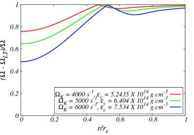
(a) along the equator

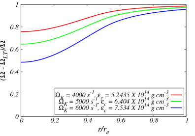
(b) along the pole

Figure 1: Frame-dragging effect inside the rotating neutron stars from the origin to the surface, calculated for the APR EoS. $\Omega_{K}$ and $\varepsilon_{c}$ denote the Kepler frequency and the central star density, respectively. Surface of the neutron star along the pole located around $0.6r_{e}$ but the plot is still valid beyond the surface of the pole as our formalism is applicable for regions outside the pulsar.

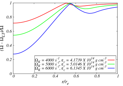
(a) along the equator

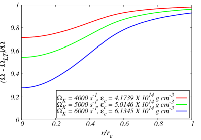
(b) along the pole

Figure 2: Same as Fig. 1, but calculated for the DD2 EoS

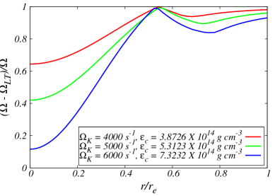
(a) along the equator

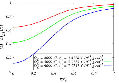
(b) along the pole

Figure 3: Same as Fig. 1, but calculated for the Chiral EoS.

The normalised frame-dragging values at the centre $(\tilde{\Omega}_{c}={\Omega_{LT}^{centre}}/{\Omega})$ and the surface $(\tilde{\Omega}_{s}={\Omega_{LT}^{surface}}/{\Omega})$ of the star models with three EoSs are recorded in Table 2.

	$P_{K}$	Along the equator			Along the pole
	(ms)	APR	DD2	Chiral	APR	DD2	Chiral
	1.57	0.008	0.013	0.019	0.046	0.069	0.099
$\tilde{\Omega}_{s}$	1.26	0.016	0.029	0.040	0.087	0.139	0.184
	1.05	0.031	0.059	0.070	0.151	0.252	0.287
	1.57	0.242	0.286	0.356	0.242	0.286	0.356
$\tilde{\Omega}_{c}$	1.26	0.354	0.457	0.580	0.354	0.457	0.580
	1.05	0.515	0.723	0.884	0.515	0.723	0.884

Table 2: Normalised angular velocities of the local inertial frame-dragging at the surface $\tilde{\Omega}_{s}$ and the centre $\tilde{\Omega}_{c}$ of the neutron stars which are rotating at their respective Kepler periods $(P_{K}\equiv 2\pi/\Omega_{K})$ as measured by a distant observer.

It is noted that the normalised frame-dragging value at the star’s center is maximum and falls off on the surfaces of the equator and pole for three EoSs irrespective of whether the compact star is rotating slowly or fast. However, for a particular EoS, the normalised frame-dragging value at the star’s centre and surface is higher for a fast rotating star with $P_{K}=1.05$ ms than those of a slowly rotating star with $P_{K}=1.57$ ms for both cases along the equator and pole. One can see another interesting thing from the Table 2 that $\tilde{\Omega}_{s}$ is always higher at the pole than $\tilde{\Omega}_{s}$ at the equator for a particular pulsar. It is due to the effect of rotation frequency $\Omega$ (of the star) for which pole is nearer to the center than the surface as it is evident from Table 2. Thus, the inertial frame-dragging effect is higher at the surface of the neutron star along the pole than that at the surface of the neutron star along the equator.

Now we investigate the dependence of local maxima and minima in $\Omega_{LT}$ along the equator on the angle $\theta$. In Figure 4, $\Omega_{LT}$ is shown as a function of $s$ defined by Eq. (21) and $\cos\theta$ for DD2 (panel(a)) and Chiral (panel (b)) EoSs. The local maxima and minima in $\Omega_{LT}$ along the equator are clearly visible in both panels of Fig. 4. It has been already noted that $\Omega_{LT}$ along the pole decreases smoothly from the center to the surface. As the latitude ($\theta^{\prime}=\pi/2-\theta$) increases from the equator to the pole, the height between the maximum and minimum of $\Omega_{LT}$ diminishes and after a certain ‘critical’ angle ($\theta_{cr}$) both extrema disappear and the plot is smooth like the plot along the pole. The critical angle could be seen from the 3-D plot in Fig. 4.

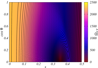
(a) $DD$2 EoS

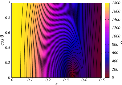
(b) APR EoS

Figure 4: 3-D plots of $\Omega_{LT}$ of the pulsar which is rotating with $\Omega_{K}=5000\,\text{s}^{-1}$ as a function of $s$ and $\cos\theta$ for (a) DD2 EoS and (b) APR EoS.

This value of the critical angle is $\mu\approx 0.5$ or $\theta_{cr}^{\prime}=30^{\circ}$ where local maximum $(r_{max})$ and minimum $(r_{min})$ disappear. So, if we plot $\Omega_{LT}$ vs $\theta$ at the point $r_{max}$ for a specific Kepler frequency, (namely $\Omega_{K}=5000\,\text{s}^{-1}$), we could find that the frame-dragging frequency increases from the equator to the pole for the specific $r_{max}$ as it is exhibited by Fig. 4.

4.2 Pulsars rotate with their frequencies $\Omega<\Omega_{K}$

Now we apply our exact formula of $\Omega_{LT}$ to three known pulsars. Three pulsars chosen for this purpose are J1807-2500B, J0737-3039A and B1257+12. Periods of those pulsars are given by Table 3. Masses of those pulsars are also known and range from 1.337 to 1.5 M_⊙. Furthermore, we adopt the same EoSs in this calculation as considered in the previous sub-section. Though periods of these pulsars are larger than the Keplerian periods, the calculation of $\Omega_{LT}$ inside these real pulsars are equally important like the cases with Kepler frequencies demonstrated already.

We calculate the normalised angular velocity at the centre and surface of these pulsars with APR, DD2 and Chiral EoSs. It is noted from Table 3 that the behaviour of the normalised angular velocity from the centre to the surface or along the pole and equator is qualitatively same as shown in Table 2.

	Name of	$P$	Along the equator			Along the pole
	the Pulsar	(ms)	APR	DD2	Chiral	APR	DD2	Chiral
	J1807-2500B	4.19	0.099	0.075	0.064	0.156	0.120	0.105
$\tilde{\Omega}_{s}$	J0737-3039A	22.70	0.095	0.073	0.062	0.154	0.122	0.106
	B1257+12	6.22	0.122	0.091	0.077	0.188	0.145	0.126
	J1807-2500B	4.19	0.707	0.548	0.516	0.707	0.548	0.516
$\tilde{\Omega}_{c}$	J0737-3039A	22.70	0.685	0.538	0.502	0.685	0.538	0.502
	B1257+12	6.22	0.825	0.632	0.601	0.825	0.632	0.601

Table 3: Normalised angular velocities of the local inertial frame-dragging at the surface $\tilde{\Omega}_{s}$ and the centre $\tilde{\Omega}_{c}$ of some known rotating neutron stars.

We also plot the frame-dragging frequency ($\Omega_{LT}$) as a function of radial distance along the equator (panel (a)) and pole (panel (b)) for three EoSs in Figures 5 - 7. The frame-dragging frequency behaves smoothly along the pole from the centre to the surface as shown by panel (b) of these figures. Results of panel (a) of the figures show similar features of local maxima and minima along the equator as found in Figs. 1-3. We note that all the local minima of $\Omega_{LT}$ are located around $r_{min}\sim 0.7r_{e}$ and the local maxima are located around $r_{max}\sim 0.9r_{e}$ in Figs. 5 - 7.

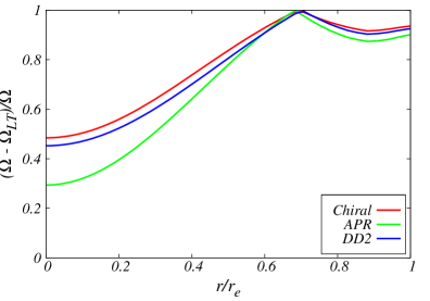
(a) along the equator

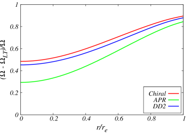
(b) along the pole

Figure 5: Frame-dragging effect inside the rotating neutron star from the origin to the surface, calculated for J1807-2500B ($M=1.366M_{\odot},\Omega=1500.935\,\text{s}^{-1}$)

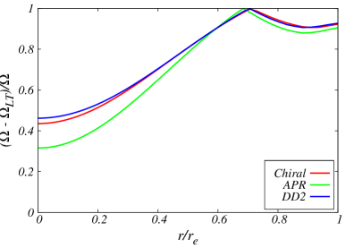
(a) along the equator

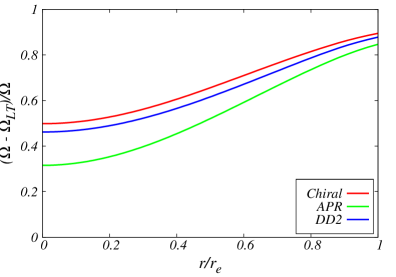
(b) along the pole

Figure 6: Frame-dragging effect inside the rotating neutron star from the origin to the surface, calculated for J0737-3039A ($M=1.337M_{\odot},\Omega=276.8\,\text{s}^{-1}$)

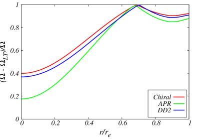
(a) along the equator

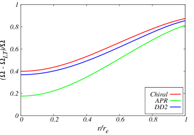
(b) along the pole

Figure 7: Frame-dragging effect inside the rotating neutron star from the origin to the surface, calculated for B1257+12 ($M=1.5M_{\odot},\Omega=1010.321\,\text{s}^{-1}$)

We also plot the $\Omega_{LT}$ of pulsar J0737-3039A as a function of $s$ and $\cos\theta$ for DD2 (panel (a)) and APR (panel (b)) EoSs in Figure 8. It is noted from Fig. 8 that the value of $\theta_{cr}$ is around $30^{\circ}$ for the pulsar J0737-3039A for DD2 and APR EoSs.

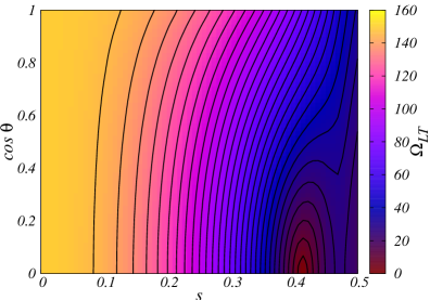
(a) $DD$2 EoS

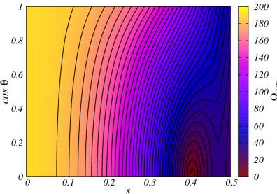
(b) APR EoS

Figure 8: 3-D plots of $\Omega_{LT}$ of the pulsar J0737-3039A as a function of $s$ and $\cos\theta$ for DD2 (panel (a)) and APR (panel (b)) EoSs.

5 Summary

We have derived the exact frame dragging frequency inside the rotating neutron star without making any assumption on the metric components and energy-momentum tensor. We show that the frequency must depend both on $r$ and $\theta$. It may be recalled that the frame-dragging frequency depends only on $r$ in Hartle’s formalism because of the slow rotation approximation. We predict the exact frame-dragging frequencies for some known pulsars as well as neutron stars rotating at their Keplerian frequencies. We have also estimated Lense-Thirring precession frequencies at the centers of these pulsars without imposing any boundary conditions on them. We have found local maxima and minima along the equator due to the dependence of $\Omega_{LT}$ on the colatitude ($\theta$) inside pulsars. The positions of local maximum and minimum depend on the frequency $\Omega$ and the central density $\varepsilon_{c}$ of the particular pulsar. Furthermore, it is observed that local maximum and minimum in $\Omega_{LT}$ along the equator disappear at a critical angle $\theta_{cr}$.

Quasi periodic oscillations (QPOs) in magnetars were studied by various groups. These studies in several cases were carried by considering spherical and non-rotating relativistic stars having dipolar magnetic field configuration (Sotani et al., 2007). It would be worth investigating this problem for rotating relativistic stars. In particular, we are studying the effect of our exact frame-dragging formulation on the magnetic field distribution in the star and its implications on QPOs. This will be published in future.

Acknowledgements: CC and KPM would like to thank Prof. Dr. P. Majumdar for various discussions regarding this project. His comments and valuable suggestions help CC a lot to make this work more appropriate. CC and KPM also thank to Mr. P. Char and Mr. A. Kheto for important discussions regarding this project. Last but not the least, CC thanks Prof. Dr. K.D. Kokkotas of University of Tübingen, Germany for gracious hospitality during an academic visit and for invaluable discussions regarding the subject of this paper. Two of us (KPM & CC) are grateful to Dept. of Atomic Energy (DAE, Govt. of India) for financial assistance.

Appendix A Appendix: Consistency check of local maximum and minimum in $\Omega_{LT}$

To find out the local maximum and minimum in $\Omega_{LT}$ we differentiate Eq.(2) with respect to $r$ and obtain

$$\frac{d{\Omega}_{LT}}{dr} = \Omega_{LT}\left[-(\alpha_{,r}+\sigma_{,r})-2\frac{r\omega\sin^{2}\theta(r\omega_{,r}+\omega)-\sigma_{,r}e^{2\sigma}}{\omega^{2}r^{2}\sin^{2}\theta-e^{2\sigma}}\right]+\frac{1}{\Omega_{LT}}.\frac{e^{-2(\alpha+\sigma)}}{4(\omega^{2}r^{2}\sin^{2}\theta-e^{2\sigma})^{2}}$$

. $$\left\{A\sin^{2}\theta\left[\omega r^{2}\sin^{2}\theta(3\omega\omega_{,r}+2r\omega_{,r}^{2}+r\omega\omega_{,rr})+2\sigma_{,r}e^{2\sigma}(2\omega+r\omega_{,r}-2\omega r\sigma_{,r})\right.\right.$$

$$+ \left.\left.e^{2\sigma}(3\omega_{,r}+r\omega_{,rr}-2r\omega_{,r}\sigma_{,r}-2\omega\sigma_{,r}-2r\omega\sigma_{,rr})\right]+B\left[r\omega\sin^{3}\theta(2\omega\omega_{,\theta}+2r\omega_{,r}\omega_{,\theta}+r\omega\omega_{,\theta r})\right.\right.$$

$$+ \left.\left.2\sigma_{,r}e^{2\sigma}(2\omega\cos\theta+\omega_{,\theta}\sin\theta-2\omega\sigma_{,\theta}\sin\theta)+e^{2\sigma}(2\omega_{,r}\cos\theta+\omega_{,\theta r}\sin\theta-2\sin\theta(\omega\sigma_{,\theta r}+\omega_{,r}\sigma_{,\theta}))\right]\right\}$$

in where

$$A = r^{3}\omega^{2}\omega_{,r}\sin^{2}\theta+e^{2\sigma}(2\omega+r\omega,_{r}-2\omega r\sigma,_{r})\,\,\,,$$ (A2)

$$B = r^{2}\omega^{2}\omega_{,\theta}\sin^{3}\theta+e^{2\sigma}(2\omega\cos\theta+\omega_{,\theta}\sin\theta-2\omega\sigma_{,\theta}\sin\theta)$$ (A3)

and

$$\omega_{,\theta r}\equiv\frac{\partial^{2}\omega}{\partial\theta\partial r}$$

Setting $\frac{d\Omega_{LT}}{dr}|_{(r=R_{0},\theta=\pi/2)}=0$ and solving it numerically in the region $0<R_{0}<r_{e}$, we obtain two positive real roots of $r$ inside the rotating neutron star. One of these is $R_{01}=r_{max}$ and another is $R_{02}=r_{min}$. These are basically the local maximum and local minimum of the function $\Omega_{LT}$ along the equator. These local maximum and local minimum are absent for $\frac{d\Omega_{LT}}{dr}|_{(r=R_{0},\theta=0)}=0$. Thus, we cannot see any such extremum for the plots of $\Omega_{LT}$ along the pole.

References

- Akmal et al. (1998) Akmal, A., Pandharipande, V. R., Ravenhall, D. G., Phys. Rev. C 58, 1804 (1998).
- Antoniadis et al. (2013) Antoniadis, J. et al. , Science 340, 1233232 (2013).
- Chakraborty & Majumdar (2014) Chakraborty, C., Majumdar, P., Class. Quantum Grav. 31, 075006 (2014).
- Chakraborty & Pradhan (2013) Chakraborty, C., Pradhan, P., Eur. Phys. J. C73, 2536 (2013).
- Cook et. al. (1992) Cook, G.B., Shapiro, S.L.,Teukolsky, S.A., ApJ 398, 203 (1992).
- Glendenning & Weber (1994) Glendenning, N. K., Weber, F., Phys. Rev. D50, 3836 (1994).
- Hartle (1967) Hartle, J.B., ApJ 150, 1005 (1967).
- Hartle (1968) Hartle, J.B., ApJ 153, 807 (1968).
- Hartle (2009) Hartle, J. B., Gravity:An Introduction to Einstein’s General relativity, Pearson (2009).
- Hanauske et al. (2000) Hanauske, M., Zschiesche, D., Pal, S., Schramm, S., Stöcker, H., Greiner, W., Astrophys. J.537, 958 (2000).
- Komatsu et. al. (1989) Komatsu, H., Eriguchi, Y., Hachisu, I., MNRAS 237, 355 (KEH) (1989).
- Lense & Thirring (1918) Lense, J., Thirring, H., Physk. Z. 19, 156 (1918).
- Morsink & Stella (1999) Morsink, S. M., Stella, L., ApJ 513, 827 (1999).
- Sotani et al. (2007) Sotani, H., Kokkotas, K. D., & Stergioulas N., MNRAS 375, 261 (2007).
- Stergioulas (1995) Stergioulas N., Friedman J.L., ApJ 444, 306 (1995).
- Typel et al. (2010) Typel, S., Röpke, G., Klähn, T., Blaschke, D., Wolter, H. H., Phys. Rev. C 81, 015803 (2010).
- Weber (1999) Weber, F., Pulsars as Astrophysical laboratories for Nuclear and Particle Physics, IOP (1999).