Spectral distances on graphs

Abstract.

By assigning a probability measure via the spectrum of the normalized Laplacian to each graph and using $L^{p}$ Wasserstein distances between probability measures, we define the corresponding spectral distances $d_{p}$ on the set of all graphs. This approach can even be extended to measuring the distances between infinite graphs. We prove that the diameter of the set of graphs, as a pseudo-metric space equipped with $d_{1}$, is one. We further study the behavior of $d_{1}$ when the size of graphs tends to infinity by interlacing inequalities aiming at exploring large real networks. A monotonic relation between $d_{1}$ and the evolutionary distance of biological networks is observed in simulations.

Keywords. Wasserstein distance, spectral measure, random rooted graph, asymptotic behavior, biological networks

AMS subject classifications. 05C50, 28A33, 05C63, 92B10

1. Introduction

One major interest in graph theory is to explore the differences of graphs in structure, that is, in the sense of graph isomorphism. In computational complexity theory, the subgraph isomorphism problem, like many combinational problems in graph theory, is NP hard. Therefore, a method that gives a quick and easy estimate of the difference between two graphs is desirable [34]. As we know, all the topological information of one graph can be found in its adjacency matrix. The spectral graph theory studies the relationship between the properties of graphs and the spectra of their representing matrices, such as adjacency matrices and Laplace matrices [14, 18, 17]. In particular, some important topological information of a graph can be extracted from its specific eigenvalue like the first or the largest one, see e.g. [18, 17, 39, 11, 25, 12, 10]. The approach of reading information from the entire spectrum of a graph was explored in [5, 6, 7, 30, 32] etc. In spite of the existence of co-spectral graphs (see [38, Chapter 3] for a general construction and the references therein), the spectra of graphs can support us one way on exploring problems that involve (sub-)graph isomorphism by the fast computation algorithms and the close relationship with the structure of graphs.

A spectral distance on the set of finite graphs of the same size, i.e. the same number of vertices, was suggested in a problem of Richard Brualdi in [37] to explore the so-called cospectrality of a graph. It was further studied in [26] using the spectra of adjacency matrices. Employing certain Gaussian measures associated to the spectra of normalized Laplacians and the corresponding $L^{1}$ distances, the first named author, Jost, the third named author and Stadler [21, 20] explored a spectral distance well-defined on the set of all finite graphs without any constraint about sizes. In this paper, instead of the Gaussian measures, we assign Dirac measures to graphs through the spectra of normalized Laplacians and use the Wasserstein distances between probability measures to propose spectral distances between graphs. In fact, this notion of spectral distances provides a metrization of the notion of spectral classes of graphs introduced in [21] via the weak convergence of the corresponding Dirac measures. The Spectral class can be considered as a weak notion of graph limits (see the concepts of graphon, graphing and related theories in the monograph of Lovász [33]). This notion of spectral distances is even adaptable for weighted infinite graphs. And we can prove diameter estimates with respect to these distances, which are sharp for certain cases.

A weighted graph $G$ is a triple $(V,E,\theta)$ where $V$ is the set of vertices, $E$ is the set of edges and $\theta:E\to(0,\infty)$, $(x,y)\mapsto\theta_{xy},$ is the (symmetric) edge weight function. We write $x\sim y$ or $xy\in E$ if $\theta_{xy}>0$. We assume that for any vertex $x,$ the weighted degree defined by $\theta_{x}:=\sum_{y\sim x}\theta_{xy}$ is finite and $\theta_{xx}=0$ (i.e. there is no self-loops).

Let us first consider finite weighted graphs. The normalized Laplacian of $G=(V,E,\theta)$ is defined as, for any function $f:V\rightarrow{\mathbb{R}}$ and any $x\in V$,

$$\Delta_{G}f(x)=f(x)-\frac{1}{\theta_{x}}\sum_{y\sim x}f(y)\theta_{xy}.$$ (1)

This operator can be extended to an infinite weighted graph which has countable vertex set $V$ but is not necessarily locally finite (see [27] or Section 2 below). As a matrix, $\Delta_{G}$ is unitarily equivalent to the Laplace matrix studied in [17].

If $x\in V$ is an isolated vertex, i.e. $\theta_{x}=0$, (1) reads as $\Delta_{G}f(x)=f(x)$. This implies that an isolated vertex contribute an eigenvalue $1$ to the spectrum of $\Delta_{G}$, denoted by $\sigma(G)$. In this way, by the absence of the self-loops, the spectrum of any finite weighted graph $\sigma(G)=\{\lambda_{i}\}_{i=1}^{N},$ counting the multiplicity, satisfies the trace condition

$$\sum_{i=1}^{N}\lambda_{i}=N$$ (2)

where $N=|V|.$ It is well-known that $\sigma(G)$ is contained in $[0,2]$. We associate to $\sigma(G)$ a probability measure on $[0,2]$ as follows:

$$\mu_{\sigma(G)}:=\frac{1}{N}\sum_{i}\delta_{\lambda_{i}},$$ (3)

where $\delta_{\lambda_{i}}$ is the Dirac measure concentrated on $\lambda_{i}.$ We call $\mu_{\sigma(G)}$ the spectral measure for a finite weighted graph. (This is known as the empirical distribution of the eigenvalues in random matrix theory.) Denote by $P([0,2])$ the set of probability measures on the interval $[0,2]$. For any $\mu\in P([0,2]),$ the first moment of $\mu$ is defined as $m_{1}(\mu):=\int_{[0,2]}\lambda\ d\mu(\lambda).$ The trace condition (2) is then translated to

$$m_{1}(\mu_{\sigma(G)})=1.$$ (4)

This is a key property of the spectral measures for our further investigations.

Let $d_{p}^{W}$ ($1\leq p<\infty$) be the $p$-th Wasserstein distance on $P([0,2])$. That is, for any $\mu$, $\nu\in P([0,2])$ (see e.g. [40]),

$$d_{p}^{W}(\mu,\nu):=\left(\inf_{\pi\in\Pi(\mu,\nu)}\int_{[0,2]\times[0,2]}d(x,y)^{p}d\pi(x,y)\right)^{1/p},$$

where $\Pi(\mu,\nu)$ denotes the collection of all measures on $[0,2]\times[0,2]$ with marginals $\mu$ and $\nu$ on the first and second factors respectively, i.e. $\pi\in\Pi(\mu,\nu)$ if and only if $\pi(A\times[0,2])=\mu(A)$ and $\pi([0,2]\times B)=\nu(B)$ for all Borel subsets $A,B\subseteq[0,2]$.

It is well-known that $(P([0,2]),d_{p}^{W})$ is a complete metric space for $p\in[1,\infty)$ which induce the weak topology of measures in $P([0,2])$(see e.g. [40, Theorem 6.9]).

One can prove that $\mathrm{diam}(P([0,2]),d_{p}^{W})=2$. Indeed, on one hand, for any $\mu,\nu\in P([0,2])$ by the optimal transport interpretation of Wasserstein distance, $d_{p}^{W}(\mu,\nu)\leq 2.$ On the other hand, $d_{p}^{W}(\delta_{0},\delta_{2})=2$. (Recall that $\delta_{0},\delta_{2}$ are the Dirac measures concentrated on $0,2$, respectively.)

Definition 1.1.

Given two finite weighted graphs $G=(V,E,\theta)$ and $G^{\prime}=(V^{\prime},E^{\prime},\theta^{\prime}),$ the spectral distance between $G$ and $G^{\prime}$ is defined as

$$d_{p}(G,G^{\prime}):=d_{p}^{W}(\mu_{\sigma(G)},\mu_{\sigma(G^{\prime})}).$$ (5)

We denote by $\mathcal{FG}$ the space of all finite weighted graphs. Then for any $1\leq p<\infty,$ $(\mathcal{FG},d_{p})$ is a pseudo-metric space. This is not a metric space due to the existence of co-spectral graphs. However, in applications this spectral consideration leads to the simplification of measuring the discrepancy of graphs.

One of the main results of our paper is the following theorem.

Theorem 1.2.

For any $1\leq p<\infty,$ we have

$$\mathrm{diam}(\mathcal{FG},d_{p})\leq 2^{1-\frac{1}{p}}.$$

Remark 1.3.

1. Embedded as a subspace of $P([0,2]),$ $\mathcal{FG}$ is a proper subspace by considering the diameters.

2. One can prove an upper bound directly by using Chebyshev inequality, see Theorem 2.4. Clearly, this theorem improves that estimate.

3. This estimate is tight for $p=1,$ i.e. $\mathrm{diam}(\mathcal{FG},d_{1})=1,$ see Corollary 1.8.

4. We don’t claim the sharpness of upper bound estimates for $p\in(1,\infty).$

In fact, Theorem 1.2 follows from the estimates on the Wasserstein distance of probability measures in condition of the first moments.

Theorem 1.4 (Measure-theoretic version).

For any $\mu,\nu\in P([0,2])$ with $m_{1}(\mu)=m_{1}(\nu)=1$ and $p\in[1,\infty),$

$$d^{W}_{p}(\mu,\nu)\leq 2^{1-\frac{1}{p}}.$$ (6)

By Proposition 2.1 and Lemma 2.2 below, one easily shows that the above measure-theoretic estimate is equivalent to the following analytic estimate.

Theorem 1.5 (Analytic version).

Let $f,g:[0,1]\to[0,2]$ be two nondecreasing functions such that $\int_{0}^{1}f(x)dx=\int_{0}^{1}g(x)dx=1.$ Then for any $p\in[1,\infty)$

$$\left(\int_{0}^{1}|f-g|^{p}(x)dx\right)^{\frac{1}{p}}\leq 2^{1-\frac{1}{p}}.$$ (7)

Section 3 is devoted to the proofs of Theorem 1.2, 1.4 and Theorem 1.5.

We extend our approach of the spectral distance to infinite graphs (with countable vertex set V) in Section 4. Note that in the above arguments we only use the normalization of the first moment of the spectral measures, i.e. $m_{1}(\mu_{\sigma(G)})=1,$ our results generalize to all weighted graphs including the infinite ones. For spectral measures with distinguished vertices on infinite graphs, we refer to Mohar-Woess [36]. We introduce two definitions of spectral measures for infinite graphs. One is defined via the exhaustion of the infinite graphs by the spectral measures of normalized Dirichlet Laplacians on subgraphs. The other is defined for random rooted graphs following Benjamini-Schramm [13], Aldous-Lyons [2] and Abért-Thom-Virág [1].

We denote by $\mathcal{G}$ the collection of all (possibly infinite) weighted graphs. For any $G\in\mathcal{G},$ we define $\mathrm{SM}(G)$ as the spectral measures of $G$ by exhaustion, see Definition 4.1, which is a closed subset of $P([0,2])$. Then $\mathcal{G}$ endowed with the Hausdorff distance induced from the metric space $(P([0,2]),d_{p}^{W})$, denoted by $d_{p,H},$ is a pseudo-metric space. A direct application of Theorem 1.4 yields the following corollary (recalled below as Theorem 4.2).

Corollary 1.6.

For $p\in[1,\infty),$

$$\mathrm{diam}(\mathcal{G},d_{p,H})\leq 2^{1-\frac{1}{p}}.$$

For any $D\geq 1,$ we denote by $\mathcal{RRG}_{D}$ the collection of random rooted graphs of degree $D,$ see Section 4.2 for definitions. Any finite weighted graph $G$ gives rise to a random graph by assigning the root of $G$ uniformly randomly. There are many interesting class of random rooted graphs such as unimodular and sofic ones, see [1]. For each random rooted graph $G\in\mathcal{RRG}_{D},$ we associate it with an expected spectral measure, denoted by $\mu_{G}.$ In this way, $\mathcal{RRG}_{D}$ endowed with $d_{p}^{W}$ Wasserstein distance for expected spectral measures ($d_{p}$ in short) is a pseudo-metric space. By Theorem 1.4, one can prove the following corollary (recalled below as Theorem 4.4).

Corollary 1.7.

For $p\in[1,\infty),$

$$\mathrm{diam}(\mathcal{RRG}_{D},d_{p})\leq 2^{1-\frac{1}{p}}.$$

In fact, there are examples of finite graphs which saturate the upper bounds for $p=1$, see Example 2.5 and 2.6.

Corollary 1.8.

All upper bounds on $d_{1}$ are tight, i.e.

$$\mathrm{diam}(\mathcal{FG},d_{1})=\mathrm{diam}(\mathcal{G},d_{1,H})=\mathrm{diam}(\mathcal{RRG}_{D},d_{1})=1.$$

We then concentrate on the spectral distance $d_{1}$. In Section 5, we calculate $d_{1}$ on several particular classes of graphs. For our purpose of application to large real networks, we are more concerned with the behavior of $d_{1}$ when the size of graphs $N$ tends to infinity. We observe convergence behaviors like $\mathcal{O}(1/N^{2})$, $\mathcal{O}(1/N)$ in those examples.

The asymptotic behavior of $d_{1}$ is studied in general in Section 6 by employing interlacing inequalities of the spectra of finite weighted graphs. For two graphs $G$ and $G^{\prime}$, which differ from each other by some standard operations including e.g. edge deleting, vertex replication, vertices contraction and edge contraction, we prove

$$d_{1}(G,G^{\prime})\leq\frac{C}{N},$$ (8)

where $C$ depends only on the operations and is independent of the size $N$ of $G$ (see Theorem 6.3). By this result, we further derive a convergence result of graphs under the $d_{1}$ distance.

In the last section, we apply the distance $d_{1}$ to study the evolutionary process of biological networks by simulations. We start from a Barabási-Albert scale-free network, which has proven to be a very common type of real large networks [8]. We then simulate the evolutionary process by the operations, edge-rewiring and duplication-divergence respectively. We observe a monotonic relation between $d_{1}$ and the evolutionary distance, which is a crucial point to anticipate further applications in exploring evolutionary history of biological networks.

2. Preliminaries, spectral measures and spectral distances

In this section, we recall basics about graph spectra and Wasserstein distances on the space of probability measures, and define the spectral distances of finite graphs. The spectral distances of infinite graphs and random graphs will be postponed to Section 4.

Let us consider a possibly infinite weighted graph $G=(V,E,\theta)$, where $V$ is a countable (possible infinite) set. We require that the weight function $\theta$ satisfies

$$\sum_{y\in V}\theta_{xy}<\infty,\qquad\forall x\in V.$$

The weighted degree of the vertex $x\in V$ is still defined as $\theta_{x}:=\sum_{y\sim x}\theta_{xy}$. The graph is called connected if for every two vertices $x,y\in V$ there exists a finite path $x=x_{0}\sim x_{1}\sim\cdots\sim x_{n}=y$ connecting $x$ and $y$.

We define the (formal) normalized Laplacian $\Delta$ on the formal domain

$$F(V):=\{f:V\to{\mathbb{R}}\mid\sum_{y\in V}\theta_{xy}|f(y)|<\infty\mbox{ for all }x\in V\},$$

by

$$\Delta f(x)=\frac{1}{\theta_{x}}\sum_{y\in V}\theta_{xy}(f(x)-f(y)).$$

As a linear operator, its restriction to the Hilbert space $\ell^{2}(V,\theta):=\{f:V\to{\mathbb{R}}|\sum_{x\in V}|f(x)|^{2}\theta_{x}<\infty\},$ denoted by $\Delta_{G}$, coincides with the generator of the Dirichlet form

$$Q(f)=\frac{1}{2}\sum_{x,y\in V}\theta_{xy}|f(x)-f(y)|^{2},$$

defined on $\ell^{2}(V,\theta),$ for details see [27].

If $G=(V,E,\theta)$ is a weighted graph without isolated vertices, i.e. $\theta_{x}>0$ for all $x\in V$, then the normalized Laplacian of $G$ can be rephrased as

$$\Delta_{G}:=I-D^{-1}A,$$

where $D$ is the degree operator and $A$ is the adjacency operator (defined as $D\tau_{x}=\theta_{x}\tau_{x}$ and $A\tau_{x}=\sum_{y\sim x}\theta_{yx}\tau_{y}$, where $\tau_{x}(y)=1$ if $y=x$ and $0$ otherwise), i.e. for any finitely supported function $f:V\to{\mathbb{R}},$

$$\Delta_{G}f(x)=f(x)-\frac{1}{\theta_{x}}\sum_{y\sim x}f(y)\theta_{xy}.$$

Since $D^{-1}A$ is a bounded selfadjoint operator with operator norm less than or equal to $1$ on $\ell^{2}(V,\theta)$, the spectrum of $\Delta_{G},$ denoted by $\sigma(G)$, is contained in the interval $[0,2].$

We order the spectrum of any finite weighted graph $G$ in the nondecreasing way:

$$0\leq\lambda_{1}\leq\cdots\leq\lambda_{N}\leq 2,$$

where $N=|V|.$ For convenience, we also denote the spectrum of $G$ by a vector, called spectral vector of $G$, $\lambda_{G}:=(\lambda_{i})_{i=1}^{N}=(\lambda_{1},\lambda_{2},\cdots,\lambda_{N})\in[0,2]^{N}.$

2.1. Spectral measures

Let $G$ be a finite weighted graph. We denote by $F_{G}$ the cumulative distribution function associated to $\mu_{\sigma(G)}$ (recall (3)), and by

$$F^{-1}_{G}(x):=\inf\{t\in{\mathbb{R}}:F_{G}(t)>x\}$$

the inverse cumulative distribution function. Since $\sigma(G)\subseteq[0,2],$ we have $F_{G}:[0,2]\to[0,1]$ and $F^{-1}_{G}:[0,1]\to[0,2]$. Recalling the trace condition (2), we have the following proposition.

Proposition 2.1.

Let $G=(V,E,\theta)$ be a finite weighted graph. Then the following are true:

1. $F_{G}$ and $F^{-1}_{G}$ are nonnegative nondecreasing step functions;

2. $\int_{0}^{2}F_{G}(x)dx=1$;

3. $\int_{0}^{1}F^{-1}_{G}(x)dx=1$.

Proof.

$(a)$ is trivial. $(c)$ follows from the trace condition (2). $(b)$ is equivalent to $(c)$ since the total area of the rectangle $[0,1]\times[0,2]$ is 2. ∎

2.2. Spectral distances

Since the spectrum of the normalized Laplacian of a graph lies in the interval $[0,2]\subset{\mathbb{R}}$, one may calculate the spectral distance (5) explicitly. This is an advantage of probability measures supported in the $1$-dimensional space. In fact, the spectral distance between two finite weighted graphs $G$, $G^{\prime}$, i.e. the Wasserstein distance of two spectral measures $\mu_{\sigma(G)},\mu_{\sigma(G^{\prime})}$, can be calculated by the inverse cumulative distribution functions $F^{-1}_{G}$ and $F^{-1}_{G^{\prime}}$ thanks to the following lemma.

Lemma 2.2 (see Theorem 8.1 in [35]).

Let $\mu,\nu\in P([0,2])$ and $F_{\mu}^{-1},F_{\nu}^{-1}$ be their inverse cumulative distribution functions. Then for any $p\in[1,\infty),$

$$d_{p}^{W}(\mu,\nu)=\left(\int_{0}^{1}|F^{-1}_{\mu}(x)-F^{-1}_{\nu}(x)|^{p}dx\right)^{1/p}.$$

One can show that if two graphs having the same number of vertices, say $N$, then the spectral distance between them is reduced to the $\ell^{p}$ distance between the spectral vectors, i.e. for any $1\leq p<\infty,$

$$d_{p}(G,G^{\prime})=\frac{1}{N}\|\lambda_{G}-\lambda_{G^{\prime}}\|_{\ell^{p}}.$$

In this paper, we are interested in the diameter of the pseudo-metric space $(\mathcal{FG},d_{p})$ for $p\in[1,\infty)$. Recall that we naturally have

$$\mathrm{diam}(\mathcal{FG},d_{p})\leq\mathrm{diam}(P([0,2]),d_{p}^{W})=2.$$

We denote by $\{\cdot\}$ a graph consisting of a single vertex without any edge. Then by our convention, $\sigma(\{\cdot\})=\{1\}.$ Clearly, for any weighted graph $G,$

$$d_{p}(G,\{\cdot\})\leq 1,\ \ \text{ for }1\leq p<\infty.$$

In the following, we use (integral) Chebyshev inequality to derive a refined upper bound for the diameter.

Lemma 2.3 (Chebyshev inequality, see [22, Section 2.17] or [19]).

For any nonnegative, monotonically increasing integrable functions $f,g:[0,1]\to[0,\infty),$ we have

$$\int_{0}^{1}f(x)g(x)dx\geq\int_{0}^{1}f(x)dx\int_{0}^{1}g(x)dx.$$ (9)

Theorem 2.4.

For any $1\leq p\leq 2,$ we have

$$\mathrm{diam}(\mathcal{FG},d_{p})\leq\sqrt{2},$$

i.e. for any finite weighted graphs $G$ and $G^{\prime},$

$$d_{p}(G,G^{\prime})\leq\sqrt{2}.$$

Proof.

Let us denote $f=F^{-1}_{G}$ and $g=F^{-1}_{G^{\prime}}.$ Then by Chebyshev inequality (9) and Proposition 2.1 (c),

$$\int_{0}^{1}fg\geq\int_{0}^{1}f\int_{0}^{1}g=1.$$

Hence, for any $1\leq p\leq 2$ we have

$$\left(\int_{0}^{1}|f-g|^{p}\right)^{2/p} \leq \int_{0}^{1}|f-g|^{2}=\int_{0}^{1}f^{2}+\int_{0}^{1}g^{2}-2\int_{0}^{1}fg$$

$$\leq 2\int_{0}^{1}f+2\int_{0}^{1}g-2=2,$$

where we have used that $f\leq 2$ and $g\leq 2.$ This proves the theorem. ∎

In the next section, we will give a tighter upper bound for the diameter estimates. In particular, in the case of $p=1,$ we derive an optimal upper bound, that is, we will prove that $\mathrm{diam}(\mathcal{FG},d_{1})=1.$ The tightness of this estimate can be seen from the following two examples.

Example 2.5.

Let $G=\{\cdot\}$ and $G^{\prime}=P_{2}$ be the path on two vertices. Then $\sigma(G^{\prime})=\{0,2\}$. Hence we have

$$d_{p}(G,G^{\prime})=1,\ \ p\in[1,\infty).$$

The following example is more convincing.

Example 2.6.

Let $G^{\prime}=P_{2}$ be the path on two vertices and $G_{N}$ an unweighted (i.e. $\theta_{xy}=1$ for every edge $xy$) complete graph on $N$ vertices. Then it is known that

$$\sigma(G_{N})=\{0,\underbrace{\frac{N}{N-1},\ldots,\frac{N}{N-1}}_{N-1}\}.$$ (10)

Therefore we have

$$d_{p}(G_{N},G^{\prime})=\left[\left(\frac{1}{2}-\frac{1}{N}\right)\frac{N^{p}}{(N-1)^{p}}+\frac{1}{2}\left(2-\frac{N}{N-1}\right)^{p}\right]^{\frac{1}{p}}.$$

In particular, $d_{1}(G_{N},G^{\prime})=1-\frac{1}{N-1}$. Observe that

$$\lim_{N\rightarrow+\infty}d_{p}(G_{N},G^{\prime})=1.$$

3. The proof of the diameter estimate

This section is devoted to the proofs of Theorem 1.2, 1.4 and Theorem 1.5. We first prove some lemmata.

We call a function $f:[0,1]\to[0,2]$ an admissible $2$-step function if there exist $a\in[0,\frac{1}{2}]$ and $b\in[\frac{1}{2},1]$ such that

$$f(x)=\left\{\begin{array}[]{ll}0,&0\leq x<a,\\ \frac{2b-1}{b-a},&a\leq x<b,\\ 2,&b\leq x\leq 1.\end{array}\right.$$ (11)

In particular, we say $f$ jumps at $a$ and $b$. Clearly, $\int_{0}^{1}f(x)dx=1$ and $\int_{0}^{2}f^{-1}(x)dx=1.$ The name for a $2$-step function is evident from the graph of the function. In particular, any inverse function $F^{-1}_{G}$ of a cumulative distribution function of a graph $G$ with $3$ vertices is an admissible $2$-step function.

Lemma 3.1.

Let $f,g$ be admissible $2$-step functions on $[0,1]$. Then we have

$$\int_{0}^{1}|f-g|(x)dx\leq 1,$$ (12)

where ”$=$” holds if and only if (ignoring the order of $f,g$)

$$f(x)=\left\{\begin{array}[]{ll}0,&\hbox{$0\leq x<\frac{1}{2}$;}\\ 2,&\hbox{$\frac{1}{2}\leq x\leq 1$,}\end{array}\right.\,\,\,g(x)=1,\,\,0\leq x\leq 1.$$ (13)

Observe that the inverse cumulative distribution functions in Example 2.5 are exactly the two functions in (13).

Proof.

Let $f:[0,1]\to[0,2]$ ($g:[0,1]\to[0,2]$ resp.) be an admissible $2$-step function jumping at $a$ and $b$ ($c$ and $d$ resp.). Denote the height of the first jump of $f$ and $g$ by $h_{1}:=\frac{2b-1}{b-a}$ and $h_{2}:=\frac{2d-1}{d-c}$ respectively.

The proof is divided into four cases and several subcases as follows:

Case 1. $0\leq a\leq c\leq\frac{1}{2}\leq d\leq b\leq 2.$

Subcase 1.1. $h_{2}\geq h_{1}.$ See Fig. 2.

For each domain I (II resp.) in Fig. 2, we denote by $|\textrm{I}|$ ($|\textrm{II}|$ resp.) the area of that domain. We reflect the domain II along the line $\{x=c\}$ to obtain a new domain $\textrm{II}^{\prime}.$ By the fact that $c\leq\frac{1}{2},$ we have

$$\int_{0}^{1}|f-g|=|\textrm{I}|+|\textrm{II}|=|\textrm{I}|+|\textrm{II}^{\prime}|\leq\int_{0}^{1}g=1.$$

Subcase 1.2. $h_{2}<h_{1}.$ See Fig. 2.

Reflect the domain I along the line $\{x=d\}$ to obtain $\textrm{I}^{\prime}.$ Then

$$\int_{0}^{1}|f-g|=|\textrm{I}|+|\textrm{II}|=|\textrm{I}^{\prime}|+|\textrm{II}|\leq\int_{0}^{2}g^{-1}(y)dy=1.$$

Figure 1. Subcase 1.1

Figure 2. Subcase 1.2

Case 2. $0\leq a\leq c\leq\frac{1}{2}\leq b<d\leq 2.$

We claim that $h_{1}\leq h_{2}.$ Suppose not, by Fig 4, we have

$$1=\int_{0}^{1}f>\int_{0}^{1}g=1,$$

which is a contradiction. This proves the claim.

Subcase 2.1. $h_{1}\geq 1,$ see Fig. 4.

Reflect the domain II along the line $\{y=h_{1}\}$ to get $\textrm{II}^{\prime}.$ Since $h_{1}\geq 1,$

$$\int_{0}^{1}|f-g|=|\textrm{I}|+|\textrm{II}|+|\textrm{III}|=|\textrm{I}|+|\textrm{II}^{\prime}|+|\textrm{III}|\leq\int_{0}^{1}f=1.$$

Figure 3. Case 2: the proof of $h_{1}\leq h_{2}$

Figure 4. Subcase 2.1

Subcase 2.2. $h_{1}<1.$ Further, we divide it into more subcases.

Subcase 2.2.1. $h_{2}\leq 1,$ see Fig. 6.

Reflect the domain II along the line $\{y=h_{2}\}$ to have $\textrm{II}^{\prime}.$ By $h_{2}\leq 1,$

$$\int_{0}^{1}|f-g|=|\textrm{I}|+|\textrm{II}|+|\textrm{III}|=|\textrm{I}|+|\textrm{II}^{\prime}|+|\textrm{III}|\leq\int_{0}^{2}g^{-1}(y)dy=1.$$

Subcase 2.2.2. $h_{2}>1.$ Moreover,

Subcase 2.2.2.1. $h_{2}-h_{1}\leq 1.$

Then by the basic estimate,

$$\int_{0}^{1}|f-g| = |\textrm{I}|+|\textrm{II}|+|\textrm{III}|=(2-h_{2})(d-b)+(h_{2}-h_{1})(b-c)+h_{1}(c-a)$$

$$\leq d-b+b-c+c-a=d-a\ \ \ \ ({\rm by}\ \max\{2-h_{2},h_{2}-h_{1},h_{1}\}\leq 1)$$

$$\leq 1.$$

Subcase 2.2.2.2. $h_{2}-h_{1}>1,$ see Fig. 6.

Reflect I along the line $\{y=h_{2}\}$ to obtain $\textrm{I}^{\prime},$ and III along the line $\{x=c\}$ to obtain $\textrm{III}^{\prime}.$ Then by the fact $h_{2}-h_{1}\geq 1\geq 2-h_{2},$ $\textrm{I}^{\prime}\cap\textrm{III}^{\prime}=\emptyset.$ Thus,

$$\int_{0}^{1}|f-g|=|\textrm{I}|+|\textrm{II}|+|\textrm{III}|=|\textrm{I}^{\prime}|+|\textrm{II}|+|\textrm{III}^{\prime}|\leq\int_{0}^{1}g=1.$$

Figure 5. Subcase 2.2.1

Figure 6. Subcase 2.2.2

Case 3. $0\leq c<a\leq\frac{1}{2}\leq b<d\leq 2.$ By interchanging the role of $a,b$ and $c,d,$ this reduces to the Case 1.

Case 4. $0\leq c<a\leq\frac{1}{2}\leq d\leq b\leq 2.$ This reduces to Case 2 by the same change as in Case 3.

Combining all the cases and subcases, we prove (12). Finally, we can check case by case that the equality in (12) can be achieved only when $f$ and $g$ are the functions given by the relation (13). This completes the proof. ∎

Before proving the next lemma, we recall some basic facts from the convex analysis. Let $\Omega$ be a convex subset of ${\mathbb{R}}^{N},$ possibly having lower Hausdorff dimension. A function $f:\Omega\to{\mathbb{R}}$ is called convex if for any $x,y\in\Omega$ and $0\leq t\leq 1,$

$$f(tx+(1-t)y)\leq tf(x)+(1-t)f(y).$$

In particular, for any norm $\|\cdot\|$ on ${\mathbb{R}}^{N}$, the function $f:{\mathbb{R}}^{N}\to{\mathbb{R}}$ defined by $f(x)=\|x-x_{0}\|$ for some fixed $x_{0}$ is a convex function. We say a point $x\in\Omega$ is extremal if it cannot be written as the nontrivial convex combination of two other points in $\Omega,$ i.e. if $x=tx_{1}+(1-t)x_{2}$ for some $0<t<1$ and $x_{1},x_{2}\in\Omega,$ then $x=x_{1}=x_{2}.$ The set of extremal points of a convex set $\Omega$ is denoted by $\mathrm{Ext}(\Omega).$ A subset $P\subset{\mathbb{R}}^{N}$ is called a (closed) convex polytope if it is the intersection of finite many half spaces, i.e. there exist $K\in{\mathbb{N}}$ linear functions $\{L_{j}\}_{j=1}^{K}$ on ${\mathbb{R}}^{N}$ such that

$$P=\bigcap_{j=1}^{K}\{x\in{\mathbb{R}}^{N}:L_{j}(x)\leq 0\}.$$

We state a well-known fact which will be used to prove the next lemma.

Fact 3.2.

Let $P$ be a compact convex polytope in ${\mathbb{R}}^{N}$ and $f:P\to{\mathbb{R}}$ a convex function. Then

$$\max_{P}f=\max_{\mathrm{Ext}(P)}f.$$ (14)

The following lemma is the special case of Theorem 1.2 when two graphs have the same number of vertices.

Lemma 3.3.

Let $N\geq 1.$ Assume that ${\alpha}=({\alpha}_{i})_{i=1}^{N}$ and ${\beta}=({\beta}_{i})_{i=1}^{N}$ satisfy $0\leq{\alpha}_{1}\leq\cdots\leq{\alpha}_{N}\leq 2$ and $0\leq{\beta}_{1}\leq\cdots\leq{\beta}_{N}\leq 2$ and

$$\|{\alpha}\|_{\ell^{1}}=\|{\beta}\|_{\ell^{1}}=N.$$

Then we have

$$\|{\alpha}-{\beta}\|_{\ell^{1}}\leq N.$$

Proof.

Let $P$ denote the compact convex polytope $\{{\alpha}\in{\mathbb{R}}^{N}:0\leq{\alpha}_{1}\leq\cdots\leq{\alpha}_{N}\leq 2,\|{\alpha}\|_{\ell^{1}}=N\}.$ Then by the induction on $N,$ one can show that the set of extremal points of $P$ is

$$\mathrm{Ext}(P)=\left\{(\underbrace{0,\cdots,0}_{k},\underbrace{a,\cdots,a}_{N-k-l},\underbrace{2,\cdots,2}_{l}):0\leq k,l\leq\frac{N}{2},a=\frac{N-2l}{N-k-l}\right\}.$$

We divide the interval $[0,1]$ equally into $N$ subintervals $\{[\frac{i-1}{N},\frac{i}{N}]\}_{i=1}^{N}.$ Then for any ${\alpha}\in P,$ we define a step function $f_{{\alpha}}:[0,1]\to[0,2]$ by

$$f_{{\alpha}}|_{[\frac{i-1}{N},\frac{i}{N}]}={\alpha}_{i}.$$

Clearly, $\int_{0}^{1}f_{{\alpha}}=\frac{1}{N}\|{\alpha}\|_{\ell^{1}}=1.$ In addition, for any $\gamma\in\mathrm{Ext}(P),$ $f_{\gamma}$ is an admissible $2$-step function defined in (11).

Note that for any fixed ${\beta}_{0}\in{\mathbb{R}}^{N},$ the function $F:{\mathbb{R}}^{N}\ni{\alpha}\mapsto\|{\alpha}-{\beta}_{0}\|_{\ell^{1}}\in{\mathbb{R}}$ is a convex function on ${\mathbb{R}}^{N}.$ We claim that

$$\max_{\begin{subarray}{c}{\alpha}\in P\\ {\beta}\in P\end{subarray}}\|{\alpha}-{\beta}\|_{\ell^{1}}=\max_{\begin{subarray}{c}\gamma\in\mathrm{Ext}(P)\\ \theta\in\mathrm{Ext}(P)\end{subarray}}\|\gamma-\theta\|_{\ell^{1}}.$$ (15)

By Fact 3.2,

$$\max_{\begin{subarray}{c}{\alpha}\in P\\ {\beta}\in P\end{subarray}}\|{\alpha}-{\beta}\|_{\ell^{1}} = \max_{{\beta}\in P}\max_{{\alpha}\in P}\|{\alpha}-{\beta}\|_{\ell^{1}}=\max_{{\beta}\in P}\max_{\gamma\in\mathrm{Ext}(P)}\|\gamma-{\beta}\|_{\ell^{1}}$$

$$= \max_{\gamma\in\mathrm{Ext}(P)}\max_{{\beta}\in P}\|\gamma-{\beta}\|_{\ell^{1}}=\max_{\gamma\in\mathrm{Ext}(P)}\max_{\theta\in\mathrm{Ext}{(P)}}\|\gamma-\theta\|_{\ell^{1}}.$$

This proves the claim.

For any $\gamma,\theta\in\mathrm{Ext}(P),$ noting that $f_{\gamma}$ and $f_{\theta}$ are admissible $2$-step functions, by Lemma 3.1, we have

$$\|\gamma-\theta\|_{\ell^{1}}=N\int_{0}^{1}|f_{\gamma}-f_{\theta}|\leq N.$$

Combining this with (15), we prove the lemma. ∎

Now we can prove Theorem 1.5. A function $f:[0,1]\to[0,2]$ is called a rationally distributed step function if there is a (rational) partition $0=r_{0}<r_{1}<r_{2}<\cdots<r_{N}=1$ with $r_{i}\in{\mathbb{Q}}$ for all $0\leq i\leq N$ and an increasing sequence $0\leq a_{1}<\cdots<a_{N}\leq 2$ such that

$$f(x)=\left\{\begin{array}[]{ll}a_{1},&0\leq x<r_{1},\\ a_{2},&r_{1}\leq x<r_{2},\\ \,\,\,\,\vdots\\ a_{N},&r_{N-1}\leq x\leq 1.\end{array}\right.$$

Proof of Theorem 1.5.

First, we consider $p=1.$ By the standard approximation argument, any such functions, $f$ and $g$, can be approximated in $L^{1}$ norm by a sequence of rationally distributed step functions, say $\{f_{n}\}_{n=1}^{\infty}$ and $\{g_{n}\}_{n=1}^{\infty},$ satisfying $\int_{0}^{1}f_{n}=\int_{0}^{1}g_{n}=1.$ Hence it suffices to prove the theorem for rationally distributed step functions.

W.l.o.g., we may assume $f$ and $g$ are rationally distributed step functions, say $f|_{[r_{i-1},r_{i}]}=a_{i}$ for $1\leq i\leq L$ and $g|_{[t_{j-1},t_{j}]}=b_{j}$ for $1\leq j\leq K$ where $L,K\in{\mathbb{N}}.$ Let $N$ denote the least common multiple of $\{m_{i}\}_{i=1}^{L}\cup\{n_{j}\}_{j=1}^{K}$ where $m_{i},n_{j}$ are the denominators of $r_{i}=\frac{c_{i}}{m_{i}}$ and $t_{j}=\frac{d_{j}}{n_{j}}$ ($c_{i},m_{i},d_{j},n_{j}\in{\mathbb{N}}$), $1\leq i\leq L,1\leq j\leq K.$ Then we have for any $1\leq p\leq N$

$$f|_{[\frac{p-1}{N},\frac{p}{N}]}={\alpha}_{p},$$

$$g|_{[\frac{p-1}{N},\frac{p}{N}]}={\beta}_{p},$$

where ${\alpha}_{p}=a_{l}$ and ${\beta}_{p}=b_{k}$ for some $1\leq l\leq L,1\leq k\leq K.$ Obviously, $0\leq{\alpha}_{1}\leq\cdots\leq{\alpha}_{N}\leq 2,$ $0\leq{\beta}_{1}\leq\cdots\leq{\beta}_{N}\leq 2$ and

$$\|{\alpha}\|_{\ell^{1}}=\|{\beta}\|_{\ell^{1}}=N.$$

Hence Lemma 3.3 implies that

$$\|{\alpha}-{\beta}\|_{\ell^{1}}\leq N.$$

That is,

$$\int_{0}^{1}|f-g|\leq 1.$$

For $p\in(1,\infty),$ it can be easily derived from the result for $p=1.$

$$\int_{0}^{1}|f-g|^{p} \leq 2^{p-1}\int_{0}^{1}|f-g|$$

$$\leq 2^{p-1}.$$

This proves the theorem.∎

Theorem 1.4 then follows directly.

Proof of Theorem 1.4.

Let $F_{\mu}$ and $F_{\nu}$ denote the cumulative distribution functions of the measures $\mu$ and $\nu$ respectively. Since the total area of the square $[0,1]\times[0,2]$ is equal to $2$, by the assumption $m_{1}(\mu)=m_{1}(\nu)=1$ we have

$$\int_{0}^{1}F_{\mu}^{-1}(x)dx=\int_{0}^{1}F_{\nu}^{-1}(x)dx=1.$$

Then our theorem follows from Theorem 1.5 and Lemma 2.2. ∎

Now we can prove Theorem 1.2.

Proof of Theorem 1.2.

This follows from Theorem 1.4 directly. ∎

4. Spectral distances of infinite graphs

In this section, we introduce two definitions of spectral measures for infinite weighted graphs with countable vertex set and extend our approach of spectral distance to this setting.

4.1. Spectral measures by exhaustion

Let $G=(V,E,\theta)$ be an infinite weighted graph and $G_{\Omega}:=(\Omega,E_{|\Omega},\theta_{|\Omega\times\Omega})$ a finite connected subgraph of $G$ induced by a subset $\Omega\subset V$. We introduce the Dirichlet boundary problem of the normalized Laplacian on $\Omega,$ see e.g. [10]. Let $\ell^{2}(\Omega,\theta)$ denote the space of real-valued functions on $\Omega$. Note that every function $f\in\ell^{2}(\Omega,\theta)$ can be extended to a function $\tilde{f}\in\ell^{2}(V,\theta)$ by setting $\tilde{f}(x)=0$ for all $x\in V\setminus\Omega$. The normalized Laplacian with the Dirichlet boundary condition on $\Omega,$ denoted by $\Delta_{G_{\Omega}},$ is defined as $\Delta_{G_{\Omega}}:\ell^{2}(\Omega,\theta)\to\ell^{2}(\Omega,\theta)$,

$$\Delta_{G_{\Omega}}f=(\Delta_{G}\tilde{f})_{|\Omega}.$$

Thus for $x\in\Omega$ the Dirichlet normalized Laplacian is pointwise defined by

$$\Delta_{G_{\Omega}}f(x)=f(x)-\frac{1}{\theta_{x}}\sum_{y\in\Omega}\theta_{xy}f(y)=\tilde{f}(x)-\frac{1}{\theta_{x}}\sum_{y\in V}\theta_{xy}\tilde{f}(y),$$

where $\theta(x)$ is the weighted degree of the entire graph. A simple calculation shows that $\Delta_{G_{\Omega}}$ is a positive self-adjoint operator. We arrange the eigenvalues of the Dirichlet Laplace operator $\Delta_{G_{\Omega}}$ in nondecreasing order, i.e. $\lambda_{1}(\Omega)\leq\lambda_{2}(\Omega)\leq\ldots\leq\lambda_{N}(\Omega)$, where $N$ is the cardinality of the set $\Omega$, i.e. $N=|\Omega|$. By the trace condition, we also have the key property

$$\sum_{i=1}^{N}\lambda_{i}(\Omega)=N.$$

As same as finite graphs, we associate it with the spectral measure,

$$\mu_{\Omega}=\frac{1}{N}\sum_{i=1}^{N}\delta_{\lambda_{i}(\Omega)}.$$

Hence $m_{1}(\mu_{\Omega})=1.$

A sequence of finite connected subgraphs $\{\Omega_{n}\}_{n=1}^{\infty}$ is called an exhaustion of the infinite graph $G$ if $\Omega_{n}\subset\Omega_{n+1}$ for all $n\in{\mathbb{N}}$ and $\cup_{n=1}^{\infty}\Omega_{n}=V.$ Hence we have a sequence of probability measures $\{\mu_{\Omega_{n}}\}_{n=1}^{\infty}$ on $[0,2].$ Since $P([0,2])$ is compact under the weak topology, up to a subsequence, w.l.o.g. we have $\mu_{\Omega_{n}}\rightharpoonup\mu$ for some $\mu\in P([0,2]).$ Note that any subsequence of an exhaustion is still an exhaustion. Therefore we define the spectral measures of an infinite graph by all possible exhaustions. Note that the convergence of the spectral structure was studied in more general setting by Kuwae-Shioya [29].

Definition 4.1.

Let $G$ be an infinite weighted graph. We define the spectral measures of $G$ by exhaustion as

$$\mathrm{SM}(G):=\{\mu\in P([0,2]):\mbox{there\ is\ an\ exhaustion}\ \{\Omega_{n}\}_{n=1}^{\infty}\ s.t.\ \mu_{\Omega_{n}}\rightharpoonup\mu\}.$$

One can show that $\mathrm{SM}(G)$ is a closed subset of $P([0,2])$. Since $m_{1}(\mu_{\Omega_{n}})=1$ for any $n\in{\mathbb{N}},$ by the weak convergence, we have $m_{1}(\mu)=1$ for any $\mu\in\mathrm{SM}(G).$

For any metric space $(X,d),$ one can define the Hausdorff distance between the subsets of $X$. For any subset $A\subset X,$ we define the distance function to the subset $A$ as $X\ni x\mapsto d(x,A)=\inf\{d(x,y)|y\in A\},$ and the $r$-neighborhood of $A$ as $U_{r}(A):=\{y\in X|d(y,A)<r\},$ $r>0.$ Given two subsets $A,B\subset X,$ the Hausdorff distance between them is defined as

$$d_{H}(A,B):=\inf\{r>0|A\subset U_{r}(B),B\subset U_{r}(A)\}.$$

One can show that the set of closed subsets of $X$ endowed with the Hausdorff distance is a metric space.

Note that for $p\in[1,\infty),$ $P([0,2])$ endowed with the $p$-th Wasserstein distance is a metric space and $\mathrm{SM}(G)$ is a closed subset of $P([0,2])$ for any weighted graph $G.$ We denote by $\mathcal{G}$ the collection of all (possibly infinite) weighted graphs. Hence $\mathcal{G}$ endowed with the Hausdorff distance induced from $(P([0,2]),d_{p}^{W})$, denoted by $d_{p,H},$ is a pseudo-metric space.

A direct application of Theorem 1.4 yields

Theorem 4.2.

For $p\in[1,\infty),$

$$\mathrm{diam}(\mathcal{G},d_{p,H})\leq 2^{1-\frac{1}{p}}.$$

4.2. Spectral measures for random rooted graphs

We follow Benjamini-Schramm [13], Aldous-Lyons [2] and Abért-Thom-Virág [1] to define random rooted graphs.

For any $D\geq 1,$ we define a subcollection of $\mathcal{G},$ $\mathcal{G}_{D}:=\{(V,E,\theta)\in\mathcal{G}|\deg_{x}\leq D,\theta_{xy}\leq D\mbox{\ for \ all\ }x,y\in V\}$ where $\deg_{x}=|\{y\in V|y\sim x\}|$, i.e. the set of weighted graphs with bounded (unweighted) degree ($\leq D$) and bounded edge weights ($\leq D$). Let $\mathcal{RG}_{D}$ denote the set of graphs $G$ in $\mathcal{G}_{D}$ with a distinguished vertex, called the root of $G.$

For any $x,y\in V$ of $G=(V,E,\theta),$ we denote by $d_{C}(x,y)$ the distance between $x$ and $y,$ i.e. $d_{C}(x,y):=\inf\{n|\mbox{\ there\ exist}\ \{x_{i}\}_{i=0}^{n}\ s.t.\ x=x_{0}\sim x_{1}\sim\cdots\sim x_{n}=y\},$ and by $B_{k}(x):=\{z\in V|d_{C}(x,z)\leq k\},$ $k\in{\mathbb{N}}\cup\{0\}$, the ball of radius $k$ centered at $x.$ Let $(G_{1},o_{1})$ and $(G_{2},o_{2})$ be two rooted graphs with distinguished vertices $o_{1}$ and $o_{2}$, respectively. We call that $B_{k}(o_{1})$ is isomorphic to $B_{k}(o_{2})$ if there exists a bijective map $f:B_{k}(o_{1})\to B_{k}(o_{2})$ such that $f(o_{1})=f(o_{2})$ and $x\sim y$ for $x,y\in B_{k}(o_{1})$ if and only if $f(x)\sim f(y).$ For $(G_{1},o_{1}),(G_{2},o_{2})\in\mathcal{RG}_{D}$ with $G_{1}=(V_{1},E_{1},\theta_{1})$ and $G_{2}=(V_{2},E_{2},\theta_{2}),$ we define the rooted distance between $G_{1}$ and $G_{2}$ as $1/K$ where

$$K=\max\{k\in{\mathbb{N}}|\ \exists\mbox{ an\ isomorphism\ }f:B_{k}(o_{1})\to B_{k}(o_{2})$$

$$\text{ such that }\ \sup_{x,y\in B_{k}(o_{1})}|\theta_{1,xy}-\theta_{2,f(x)f(y)}|\leq\frac{1}{k}\},$$

$\theta_{1,xy},\theta_{2,f(x)f(y)}$ are edge weights of $xy\in E_{1}$, $f(x)f(y)\in E_{2}$, respectively. One can prove that $\mathcal{RG}_{D}$ endowed with the rooted distance is a compact metric space.

By a random rooted graph of degree $D$ we mean a Borel probability distribution on $\mathcal{RG}_{D}.$ We denote by $\mathcal{RRG}_{D}$ the collection of random rooted graphs of degree $D.$ Any finite weighted graph $G$ gives rise to a random rooted graph by assigning the root of $G$ uniformly randomly.

For a rooted weighted graph $(G,o)\in\mathcal{RG}_{D}$ with $G=(V,E,\theta),$ the normalized Laplacian is a bounded self-adjoint operator on $\ell^{2}(V,\theta)$ which is independent of $o.$ By spectral theorem, there is a projection-valued measure, denoted by $P_{\bullet},$ on $[0,2],$ i.e. $P_{A}$ is a projection on $\ell^{2}(V,\theta)$ for any Borel $A\subset[0,2],$ such that for any continuous function $f\in C([0,2])$ we have the functional calculus

$$f(\Delta_{G})=\int_{[0,2]}f(x)dP_{x}$$ (16)

where $P_{x}=P_{[0,x]}.$ We define the spectral measure of the rooted graph $(G,o)$ as

$$\mu_{G,o}=\frac{1}{\theta_{o}}\langle P_{A}\delta_{o},\delta_{o}\rangle,\ \ \forall A\subset[0,2],$$

where $\langle\cdot,\cdot\rangle$ is the inner product for $\ell^{2}(V,\theta).$ One can easily show that $\mu_{G,o}$ is a probability measure on $[0,2]$. Further calculation by using (16) yields $m_{1}(\mu_{G,o})=1.$ Now we can define the expected spectral measure for rooted random graphs.

Definition 4.3.

Let $G$ be a random rooted graph. We define the expected spectral measure of $G$ as

$$\mu_{G}=E(\mu_{G,o})$$

where the expectation is taken over the distribution on $\mathcal{RG}_{D}.$

Let $G$ be a random rooted graph rising from a finite weighted graph with uniform distribution on its vertices. A similar calculation as in Abért-Thom-Virág [1] shows that

$$\mu_{G}=\frac{1}{N}\sum_{i=1}^{N}\delta_{\lambda_{i}}$$

where $\{\lambda_{i}\}_{i=1}^{N}$ is the spectrum of the finite graph. Hence the expected spectral measure of random rooted graphs generalizes the spectral measure of finite graphs. There are other interesting classes of random rooted graphs such as unimodular and sofic ones, see e.g. [1].

The set of random rooted graphs of degree $D,$ $\mathcal{RRG}_{D}$, endowed with $d_{p}^{W}$ Wasserstein distance for expected spectral measures ($d_{p}$ in short) is a pseudo-metric space. By Theorem 1.4, one can prove the following theorem.

Theorem 4.4.

For $p\in[1,\infty),$

$$\mathrm{diam}(\mathcal{RRG}_{D},d_{p})\leq 2^{1-\frac{1}{p}}.$$

5. Calculation of examples

From now on, we will concentrate on the study of the spectral distance $d_{1}$. We calculate this distance for several classes of graphs in this section. Rather than the exact value of the $d_{1}$ distance between two graphs, we are more concerned with the asymptotical behavior of the distance between two sequences of graphs which become larger and larger, as the sizes of real networks in practice nowadays are typically huge. All example graphs we consider in this section are unweighted.

Proposition 5.1.

For two complete graphs $G$ and $G^{\prime}$ with $N$ and $M$ ($M>N$) vertices respectively, we have

$$d_{1}(G,G^{\prime})=2\frac{M-N}{N(M-1)}.$$

Proof.

Recall the spectrum (10) of a complete graph. We then calculate the distance (i.e. the area of the grey region shown in Fig. 7),

$$d_{1}(G,G^{\prime})=\frac{M}{M-1}\left(\frac{1}{N}-\frac{1}{M}\right)+\left(\frac{N}{N-1}-\frac{M}{M-1}\right)\left(1-\frac{1}{N}\right)=2\frac{M-N}{N(M-1)}.$$

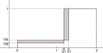
Figure 7. Two complete graphs of size $N$ and $M$

∎

Remark 5.2.

When the size difference $M-N$ of two complete graphs is a fixed constant $C$, we have

$$d_{1}(G,G^{\prime})=\mathcal{O}(1/N^{2})\text{ as }N\rightarrow\infty.$$

Proposition 5.3.

For two connected complete bipartite graphs $G$ and $G^{\prime}$ of size $N$ and $M$ ($M>N$) respectively, we have

$$d_{1}(G,G^{\prime})=2\frac{M-N}{NM}.$$

Proof.

The spectrum of a complete bipartite graph $G$ with $N$ vertices is

$$\sigma(G)=\{0,\underbrace{1,\ldots,1}_{N-2},2\}.$$

Then the distance is (the area of the grey region shown in Fig. 8)

$$d_{1}(G,G^{\prime})=\left(\frac{1}{N}-\frac{1}{M}\right)+\left(\frac{M-1}{M}-\frac{N-1}{N-1}\right)=2\frac{M-N}{NM}.$$

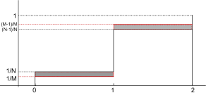
Figure 8. Two complete bipartite graphs of size $N$ and $M$

∎

Remark 5.4.

If the size difference $M-N$ of two complete bipartite graphs is a fixed constant $C$, we again observe the behavior

$$d_{1}(G,G^{\prime})=\mathcal{O}(1/N^{2})\text{ as }N\rightarrow\infty.$$

Proposition 5.5.

For two cubes $G$ and $G^{\prime}$ of size $2^{N}$ and $2^{N+1}$ respectively, we have

$$d_{1}(G,G^{\prime})=\frac{1}{N+1}.$$

Proof.

The spectrum of the cube $G$ with $2^{N}$ vertices is

$$\left\{\frac{2i}{N}\text{ with multiplicity }\binom{N}{i},i=0,\ldots,N\right\}.$$

Firstly, observe $\frac{2i}{N}=\frac{2j}{N+1}$ when $i=j=0$ or $i=N$, $j=N+1$. And for $j=i$, we have

$$\frac{2(i-1)}{N}<\frac{2j}{N+1}<\frac{2i}{N},\text{ for }1\leq i\leq N.$$

Secondly, by the recursive formula $\binom{N+1}{k}=\binom{N}{k-1}+\binom{N}{k}$, for $1\leq k\leq N$, we derive

$$\frac{1}{2^{N+1}}\sum\limits_{i=0}^{k}\binom{N+1}{i}<\frac{1}{2^{N}}\sum\limits_{i=0}^{k}\binom{N}{i}<\frac{1}{2^{N+1}}\sum\limits_{i=0}^{k+1}\binom{N+1}{i},\text{ for }0\leq k\leq N-1.$$

Therefore the distance between $G$ and $G^{\prime}$ equals the area of the grey region depicted in Fig. 9.

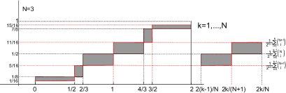
Figure 9. An example of two neighboring cubes with $N=3$ and $N+1=4$.

Again by the recursive formula of binomial numbers, we calculate,

$$d_{1}(G,G^{\prime}) = \sum\limits_{k=1}^{N}\Bigg{\{}\left(\frac{2k}{N+1}-\frac{2(k-1)}{N}\right)\left[\frac{1}{2^{N}}\sum\limits_{i=0}^{k-1}\binom{N}{i}-\frac{1}{2^{N+1}}\sum\limits_{i=0}^{k-1}\binom{N+1}{i}\right]$$

$$+\left(\frac{2k}{N}-\frac{2k}{N+1}\right)\left[\frac{1}{2^{N+1}}\sum\limits_{i=0}^{k}\binom{N+1}{i}-\frac{1}{2^{N}}\sum\limits_{i=0}^{k-1}\binom{N}{i}\right]\Bigg{\}}$$

$$= \frac{1}{2^{N}N(N+1)}\Bigg{\{}\sum\limits_{k=1}^{N}(N-k+1)\left[2\sum\limits_{i=0}^{k-1}\binom{N}{i}-\sum\limits_{i=0}^{k-1}\binom{N+1}{i}\right]$$

$$+k\left[\sum\limits_{i=0}^{k}\binom{N+1}{i}-2\sum\limits_{i=0}^{k-1}\binom{N}{i}\right]\Bigg{\}}$$

$$= \frac{1}{2^{N}N(N+1)}\sum\limits_{k=1}^{N}\left[(N-k+1)\binom{N}{k-1}+k\binom{N}{k}\right]$$

$$= \frac{2}{2^{N}N(N+1)}\sum\limits_{k=1}^{N}k\binom{N}{k}=\frac{2}{2^{N}N(N+1)}\cdot N\cdot 2^{N-1}=\frac{1}{N+1}.$$

∎

Remark 5.6.

The distance between two neighboring cubes ($N$-cube and $(N+1)$-cube) is $\mathcal{O}(1/N)$ as $N$ tends to infinity. Recall a crucial difference of this example from previous ones is that the size difference, $2^{N}$, is not uniformly bounded as $N\rightarrow\infty$.

Proposition 5.7.

For two paths $G$ and $G^{\prime}$ of size $N$ and $N+1$ respectively, we have

$$d_{1}(G,G^{\prime})=\frac{1}{N(N+1)}\left(\cot^{2}{\frac{\pi}{2N}}-\cot^{2}{\frac{\pi}{2(N-1)}}+1\right)$$

Proof.

The spectrum of the path $G$ with with $N$ vertices is

$$\left\{1-\cos{\frac{\pi i}{N-1}},i=0,1,\ldots,N-1\right\}.$$

Since $1-\cos\frac{i\pi}{N-1}<1-\cos\frac{(i+1)\pi}{N}<1-\cos\frac{(i+1)\pi}{N-1}$ for $i=0,\ldots,N-2$, and every eigenvalue of a path has multiplicity one, the situation is similar to Proposition 5.5, as shown in Fig. 10.

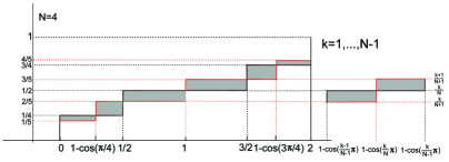
Figure 10. An example of two neighboring paths with $N=4$ and $N+1=5$.

$$d_{1}(G,G^{\prime}) = \sum\limits_{k=1}^{N-1}\bigg{\{}\left(\cos{\frac{k-1}{N-1}\pi}-\cos{\frac{k}{N}\pi}\right)\left(\frac{k}{N}-\frac{k}{N+1}\right)$$

$$+\left(\cos{\frac{k}{N}-\cos{\frac{k}{N-1}\pi}\pi}\right)\left(\frac{k+1}{N+1}-\frac{k}{N}\right)\bigg{\}}$$

$$= \frac{2}{N(N+1)}\sum\limits_{k=1}^{N-1}k\left(\cos{\frac{k-1}{N-1}\pi}-\cos{\frac{k}{N}\pi}\right)\hskip 127.48703pt$$

$$= \frac{1}{N(N+1)}\left(\cot^{2}{\frac{\pi}{2N}}-\cot^{2}{\frac{\pi}{2(N-1)}}+1\right).$$

For the last equality above we use the Lagrange’s trigonometric identities

$$\sum_{k=1}^{N}\sin kx=\frac{\cos\frac{1}{2}x-\cos(n+\frac{1}{2})x}{2\sin\frac{1}{2}x},\,\,\sum_{k=1}^{N}\cos kx=\frac{\sin(n+\frac{1}{2})x-\sin\frac{1}{2}x}{2\sin\frac{1}{2}x},$$

and their derivatives. ∎

Remark 5.8.

By a Taylor expansion argument, we observe that

$$\cot^{2}{\frac{\pi}{2N}}-\cot^{2}{\frac{\pi}{2(N-1)}}=\mathcal{O}(N),\,\,\text{ as }N\rightarrow+\infty.$$

Therefore in this example, we have $d_{1}(G,G^{\prime})=\mathcal{O}(1/N)$ as $N$ tends to infinity.

We can calculate the example of cycles similarly.

Proposition 5.9.

For two cycles $G$ and $G^{\prime}$ of size $N$ and $N+1$ respectively, we have

$$d_{1}(G,G^{\prime})=\left\{\begin{array}[]{ll}\frac{1}{N}+\frac{1}{N(N+1)}\left(\frac{1}{1-\cos(\frac{\pi}{N+1})}-\frac{4}{1-\cos(\frac{2\pi}{N})}\right),&\hbox{if $N$ is even;}\\ \frac{1}{N+1}-\frac{1}{N(N+1)}\left(\frac{1}{1-\cos(\frac{\pi}{N})}-\frac{4}{1-\cos(\frac{2\pi}{N+1})}\right),&\hbox{if $N$ is odd.}\end{array}\right.$$

Remark 5.10.

For $N$- and $(N+1)$-cycles, we also have $d_{1}(G,G^{\prime})=\mathcal{O}(1/N)$ as $N$ tends to infinity.

6. Distance between large graphs

In this section we explore the behaviors of the spectral distance $d_{1}$ between large graphs in general. We require two large graphs are different from each other only by finite steps of operations which will be made clear in Remark 6.1. The main tool we employ is the so-called interlacing inequalities, which describe the changes of the spectrum when we perform some operations on the underlying graph. Such kind of results for normalized Laplacian of a graph have been studied in [16, 31, 15, 23, 3]. In fact, we can observe the interlacing phenomena of eigenvalues for paths and cycles in Proposition 5.7 and 5.9.

Let the cardinality of vertices of $G$ and $G^{\prime}$ be $N$ and $N-j$ respectively, where $j\in\mathbb{Z}$ can be either negative or positive. Assume

$$0\leq\lambda_{1}\leq\lambda_{2}\leq\cdots\leq\lambda_{N}\text{ and }0\leq\lambda^{\prime}_{1}\leq\lambda^{\prime}_{2}\leq\cdots\leq\lambda^{\prime}_{N-j}$$

are the spectra of the corresponding normalized Laplacian $\Delta_{G}$ and $\Delta_{G^{\prime}}$. Then interlacing inequalities have the following general form.

$$\lambda_{i-k_{1}}\leq\lambda^{\prime}_{i}\leq\lambda_{i+k_{2}},\text{ for each }i=1,2,\ldots,N-j,$$ (17)

with the notation that $\lambda_{i}=0$ for $i\leq 0$ and $\lambda_{i}=2$ for $i>N$, and $k_{1},k_{2}$ are constants independent of the index $i$.

Remark 6.1.

$G^{\prime}$ can be obtained from $G$ by performing the following operations.

• $G^{\prime}$ is the proper difference of $G$ and one of its subgraph $L$. We say $L$ is a subgraph of $G$ if the weights $\theta_{L,uv}\leq\theta_{G,uv}$ for all $u,v$. And the proper difference of $G$ and $L$ is a weighted graph with weights $\theta_{G}-\theta_{L}$. In this case,

  $$k_{1}=\text{number of vertices in }L-\text{number of connected components of }L$$

  and

  $$k_{2}=\text{number of vertices in }L$$

  (Horak-Jost [23, Corollary 2.11], see also Butler [15]). This includes the operation of deleting an edge (see Chen et al [16] for the result for this particular operation). Symmetrically, this also covers the operation of adding a graph, see Bulter [15] for particular results and Atay-Tunçel [3] for vertex replication.

• $G^{\prime}$ is the image of an edge-preserving map $\varphi:G\rightarrow G^{\prime}$. By an edge-preserving map here we mean an onto map from the vertices of $G$ to vertices of $G^{\prime}$, such that

  $$\theta_{H,xy}=\sum_{\begin{subarray}{c}u\in\varphi^{-1}(x)\\ v\in\varphi^{-1}(y)\end{subarray}}\theta_{G,uv}$$

  for all vertices $x,y$ of $G^{\prime}$, and the degree of vertices are defined according to the edge weights as usual in both graphs. Notice that for our purpose, we do not allow $\varphi$ maps two neighboring vertices in $G$ to the same vertex in $G^{\prime}$ in order to avoid self-loops. In this case,

  $$k_{1}=0\text{ and }k_{2}=j.$$

  (Horak-Jost [23, Theorem 3.8].) This includes the operation of contracting vertices $u,v$ such that $N(u)\cap(N(v)\cup\{v\})=\emptyset$ (see Chen et al. [16]), where $N(u)$ stands for the neighborhood of $u$.

• $G^{\prime}$ is obtained from $G$ by contracting an edge. We only consider edges $uv$ in $G$ such that $d_{u},d_{v}>1$. By edge contracting we mean deleting the edge $(u,v)$ and identifying $u$ and $v$ (Horak-Jost [23, Definition 4.2]). Denote the number of common neighbors of $u,v$ by $m$. Then

  $$\text{when }m\neq 0,k_{1}=2m,k_{2}=1+2m;\text{ when }m=0,k_{1}=0,k_{2}=2.$$

  (Horak-Jost [23, Theorem 4.1], where the unweighted normalized Laplacian case was discussed. We do not know whether it is also true for weighted normalized Laplacian.)

Remark 6.2.

To the knowledge of the authors, the above three classes of operations includes all the operations discussed in the literature for interlacing results of normalized Laplacian.

We prove the following result.

Theorem 6.3.

Let $G$, $G^{\prime}$ be two graphs, for which the spectra of corresponding normalized Laplacians satisfy (17). Then we have

$$d_{1}(G,G^{\prime})\leq C(k_{1},k_{2},j)\frac{1}{N}.$$ (18)

Proof.

By definition, we have

$$d_{1}(G,G^{\prime})=d_{1}^{W}\left(\frac{1}{N}\sum_{i=1}^{N}\delta_{\lambda_{i}},\frac{1}{N+j}\sum_{i+1}^{N+j}\delta_{\lambda^{\prime}_{i}}\right).$$

By symmetry, w.l.o.g., we can suppose $j\geq 0$. We use a particular transport plan to derive the upper bound estimate. We move the mass $\frac{1}{N}$ from $\lambda_{i}$ to $\lambda^{\prime}_{i}$ for $i=1,2,\ldots,N-j$. We then move the mass at the remaining positions $\lambda_{N-j+1},\ldots,\lambda_{N}$ to fill the gaps at $\lambda^{\prime}_{1},\lambda^{\prime}_{2},\ldots,\lambda^{\prime}_{N-j}$ with a cost for every transportation at most $2$. That is, we have

$$d_{1}(G,G^{\prime}) \leq\frac{1}{N}\sum_{i=1}^{N-j}|\lambda_{i}-\lambda^{\prime}_{i}|+\frac{j}{N}\times 2$$

$$\leq\frac{1}{N}\sum_{i=1}^{N+j}|\lambda_{i+k_{2}}-\lambda_{i-k_{1}}|+\frac{2j}{N}$$

$$\leq\frac{k_{1}+k_{2}+1}{N}\sum_{i=1}^{N}|\lambda_{i+1}-\lambda_{i}|+\frac{2j}{N}$$

$$\leq 2(k_{1}+k_{2}+j+1)\frac{1}{N}.$$

In the second inequality above, we used interlacing inequalities (17). This complete the proof. ∎

Remark 6.4.

The disjoint union of a path of size $N$ and an isolated vertex can be obtained from a path of size $N+1$ by deleting an edge. A cycle of size $N$ can be obtained from a cycle of size $N+1$ by contracting an edge. Recall our calculation in Proposition 5.7 and 5.9, we see the estimate (18) is sharp in the order of $1/N$.

Remark 6.5.

This theorem tells that if two large graphs share similar structure, then the spectral distance between them is small.

If $G^{\prime}$ is the graph obtained from $G$ by performing operations such that $k_{1},k_{2}$ are bounded (then $j$ is also bounded), we say $G^{\prime}$ differs from $G$ by a bounded operation.

Corollary 6.6.

Let $\{G_{i}\}_{i=1}^{\infty}$ be a sequence of graphs with size $N_{i}$ tending to infinity. Assume that for any $i$, $G^{\prime}_{i}$ differs from $G_{i}$ by a uniformly bounded operation, then

$$\lim_{i\rightarrow\infty}d_{1}(G_{i},G^{\prime}_{i})=0.$$

7. Applications to biological networks

In real biological networks, such as protein interaction networks, edge-rewiring and duplication-divergence are two edit operations which have been proven to be closely related to some evolutionary mechanism, see [24, 28]. For a spectral analysis of the effect of such operations on protein interaction networks, we refer to [4]. In this section, we apply the spectral distance $d_{1}$ to capture evolutionary signals in protein interaction networks through detecting their structural differences. We evolve graphs by operations of edge-rewiring and duplication-divergence, and then check the connection between the spectral distance $d_{1}$ and the evolutionary distance (i.e. the number of evolutionary operation steps). We restrict our simulations in the following to unweighted graphs.

Let us first explain the two edit operations on an unweighted graph $G=(V,E)$ explicitly.

• Edge-rewiring: Select randomly two edges $v_{1}v_{3}$, $v_{4}v_{5}\in E$ on four distinct vertices $v_{1}$, $v_{3}$, $v_{4}$, $v_{5}\in V$ (see Fig. 11(a)). Delete these two edges $v_{1}v_{3}$, $v_{4}v_{5}$ and add new edges $v_{1}v_{4}$, $v_{3}v_{5}$. The size of the graph is preserved by this operation, and so is the degree sequence.

• Duplication-divergence: Select randomly a target vertex $v_{3}\in V$. Add a replica $v_{2}$ of $v_{3}$ and new potential edges connecting $v_{2}$ with every neighbor of $v_{3}$. Each of these potential edges is activated with certain probability (0.5 in our simulations). Then if at least one of these potential edges is established, keep the replica $v_{2}$; otherwise, delete the replica $v_{2}$ (see Fig. 11(b)).

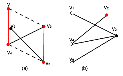
Figure 11. (a) Edge-rewiring; (b) Duplication-divergence.

Our simulations are designed as follows. We start form a Barabási-Albert scale-free graph with $1000$ vertices. This is obtained through a mechanism incorporating growth and preferential attachment from a small complete graph of size $10$, see [8, 9]. For each step of preferential attachment, we add one vertex with two edges. We remark that the Barabási-Albert scale-free graph is not necessarily the best starting model for any biological network. However, it is closer to biological networks in many cases than the other two popular models, the Erdős-Rényi random graph and the Watts-Strogatz small-world graph. Therefore, we use it as our starting point here. We carry out the operation of edge-rewiring and duplication-divergence on this graph iteratively, then plot the relationship of the spectral distance and the evolutionary distance between new obtained graphs and the original ones.

In the plot of Fig. 12, we observe that the spectral distance between graphs obtained by edge-rewiring operations and the original one increases more quickly than that obtained by duplication-divergence operations. This indicates that, after the same number of operation steps, edge-rewiring brings in more randomness to the graph than duplication-divergence. Recall also the fact that the sizes of graphs are invariant in the former case and vary in the later case.

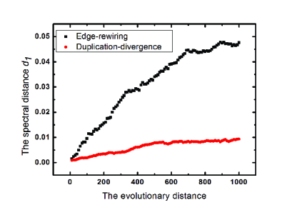
Figure 12. The relation between the spectral distance $d_{1}$ and the evolutionary distance. Edit operations includes (a) edge-rewiring; (b) duplication-divergence.

Although there is no strictly linear relation between the two distances, the spectral distance increases monotonically with respect to the evolutionary distance. Based on this crucial point, the spectral distance is very useful for exploring the hiding evolutionary history of large real networks.

References

- [1] M. Abért, A. B. Thom, B. Virág, Benjamini-Schramm convergence and pointwise convergence of the spectral measure, preprint.
- [2] D. Aldous, R. Lyons, Processes on unimodular random networks, Electron. J. Probab. 12 (2007), no. 54, 1454-1508.
- [3] F. M. Atay, H. Tunçel, On the spectrum of the normalized Laplacian for signed graphs: Interlacing, contraction, and replication, Linear Algebra Appl. 442 (2014), 165-177.
- [4] A. Banerjee, J. Jost, Laplacian spectrum and protein-protein interaction networks, arXiv: 0705:3373, 2007.
- [5] A. Banerjee, J. Jost, Spectral plot properties: towards a qualitative classification of networks, Netw. Heterog. Media 3 (2008), no. 2, 395-411.
- [6] A. Banerjee, J. Jost, On the spectrum of the normalized graph Laplacian, Linear Algebra Appl. 428 (2008), no. 11-12, 3015-3022.
- [7] A. Banerjee, J. Jost, Graph spectra as a systematic tool in computational biology, Discrete Appl. Math. 157 (2009), no. 10, 2425-2431.
- [8] A.-L. Barabási and R. Albert, Emergence of scaling in random networks, Science 286 (1999), no. 5439, 509-512.
- [9] A.-L. Barabási, E. Bonabeau, Scale-Free networks, Scientific American, 2003.
- [10] F. Bauer, B. Hua, J. Jost, The dual Cheeger constant and spectra of infinite graphs, Adv. Math. 251 (2014), 147-194.
- [11] F. Bauer, J. Jost, Bipartite and neighborhood graphs and the spectrum of the normalized graph Laplacian, Comm. Anal. Geom. 21 (2013), no. 4, 787-845.
- [12] F. Bauer, J. Jost, S. Liu, Ollivier-Ricci curvature and the spectrum of the normalized graph Laplace operator, Math. Res. Lett. 19 (2012), no. 6, 1185-1205.
- [13] I. Benjamini, O. Schramm, Recurrence of distributional limits of finite planar graphs, Electron. J. Probab. 6 (2001), no. 23, 13 pp.
- [14] N. Biggs, Algebraic graph theory, Second edition, Cambridge Mathematical Library, Cambridge University Press, Cambridge, 1993.
- [15] S. Butler, Interlacing for weighted graphs using the normalized Laplacian. Electron. J. Linear Algebra 16 (2007), 90-98.
- [16] G. Chen, G. Davis, F. Hall, Z. Li, K. Patel, M. Stewart, An interlacing result on normalized Laplacians, SIAM J. Discrete Math. 18 (2004), no. 2, 353-361.
- [17] F. R. K. Chung, Spectral graph theory, CBMS Regional Conference Series in Mathematics 92, American Mathematical Society, Providence, RI, 1997.
- [18] D. Cvetković, M. Doob, H. Sachs, Spectra of graphs, Theory and applications, Third edition, Johann Ambrosius Barth, Heidelberg, 1995.
- [19] A. M. Fink, M. Jr. Jodeit, On Chebyshev’s other inequality, Inequalities in statistics and probability (Lincoln, Neb., 1982), 115-120, IMS Lecture Notes Monogr. Ser., 5, Inst. Math. Statist., Hayward, CA, 1984.
- [20] J. Gu, The spectral distance based on the normalized Laplacian and applications to large networks, PhD Thesis, University of Leipzig, 2014.
- [21] J. Gu, J. Jost, S. Liu, P. F. Stadler, Spectral classes of regular, random, and empirical graphs, arXiv: 1406.6454, 2014.
- [22] G. H. Hardy, J. E. Littlewood, G. Pólya, Inequalities, 2d ed. Cambridge, at the University Press, 1952.
- [23] D. Horak, J. Jost, Interlacing inequalities for eigenvalues of discrete Laplace operators, Ann. Global Anal. Geom. 43 (2013), no. 2, 177-207.
- [24] I. Ispolatov, P. L. Krapivsky, A. Yuryev, Duplication-divergence model of protein interaction network, Phys. Rev. E 71 (6):061911, 2005.
- [25] J. Jost, S. Liu, Ollivier’s Ricci curvature, local clustering and curvature dimension inequalities on graphs, Discrete Comput. Geom. 51 (2014), no. 2, 300-322.
- [26] I. Jovanović, Z. Stanić, Spectral distances of graphs, Linear Algebra Appl. 436 (2012), no. 5, 1425-1435.
- [27] M. Keller, D. Lenz, Dirichlet forms and stochastic completeness of graphs and subgraphs, J. Reine Angew. Math. 666 (2012), 189-223.
- [28] J. Kim, I. Kim, S. K. Han, J. U. Bowie, S. Kim, Network rewiring is an important mechanism of gene essentiality change, Scientific reports, 2 (2012).
- [29] K. Kuwae, T. Shioya, Convergence of spectral structures: a functional analytic theory and its applications to spectral geometry, Comm. Anal. Geom. 11 (2003), no. 4, 599-673.
- [30] J. R. Lee, S. Oveis Gharan, L. Trevisan, Multi-way spectral partitioning and higher-order Cheeger inequalities, STOC’12-Proceedings of the 2012 ACM Symposium on Theory of Computing, 1117-1130, ACM, New York, 2012; J. ACM 61 (2014), no. 6, 37:1-30.
- [31] C.-K. Li, A short proof of interlacing inequalities on normalized Laplacians, Linear Algebra Appl. 414 (2006), no. 2-3, 425-427.
- [32] S. Liu, Multi-way dual Cheeger constants and spectral bounds of graphs, Adv. Math. 268 (2015), 306-338.
- [33] L. Lovász, Large networks and graph limits, American Mathematical Society Colloquium Publications, 60, American Mathematical Society, Providence, RI, 2012.
- [34] O. Macindoe, W. Richards, Graph comparison using fine structure analysis, SOCIALCOM ’10 Proceedings of the 2010 IEEE Second International Conference on Social Computing, Pages 193-200, IEEE Computer Society Washington, DC, USA, 2010.
- [35] P. Major, On the invariance principle for sums of independent identically distributed random variables, J. Multivariate Anal. 8 (1978), no. 4, 487-517.
- [36] B. Mohar, W. Woess, A survey on spectra of infinite graphs, Bull. London Math. Soc. 21 (1989), no. 3, 209-234.
- [37] D. Stevanović, Research problems from the Aveiro Workshop on graph spectra, Linear Algebra Appl. 423 (2007), no. 1, 172-181.
- [38] M. Thüne, Eigenvalues of matrices and graphs, PhD Thesis, University of Leipzig, 2012.
- [39] L. Trevisan, Max cut and the smallest eigenvalue, STOC’09-Proceedings of the 2009 ACM International Symposium on Theory of Computing, 263-271, ACM, New York, 2009; SIAM J. Comput. 41 (2012), no. 6, 1769-1786.
- [40] C. Villani, Topics in optimal transportation, Graduate Studies in Mathematics, 58. American Mathematical Society, Providence, RI, 2003.