Cyclic representations of the periodic Temperley Lieb algebra,
complex Virasoro representations and stochastic processes

Abstract

An $N$${L}\choose{L/2}$ dimensional representation of the periodic Temperley-Lieb algebra $TL_{L}(x)$ is presented. It is also a representation of the cyclic group $Z_{N}$. We choose $x=1$ and define a Hamiltonian as a sum of the generators of the algebra acting in this representation. This Hamiltonian gives the time evolution operator of a stochastic process. In the finite-size scaling limit, the spectrum of the Hamiltonian contains representations of the Virasoro algebra with complex highest weights. The $N=3$ case is discussed in detail. One discusses shortly the consequences of the existence of complex Virasoro representations on the physical properties of the systems.

The periodic Temperley-Lieb algebra $PTL_{L}(x)$ was introduced by Levy LEV in 1991 in order to explain some regularities observed in the spin 1/2 XXZ quantum chain with periodic boundary conditions AGR . The algebra has $L$ generators and depends on a parameter $x$. Various quotients of this algebra were studied by Martin and Saleur MAS . A renewed interest in the $PTL_{L}(x)$ appeared in the last few years in the context of logarithmic conformal field theory MPR and GSR . Lately stochastic processes describing nonlocal asymmetric exclusion processes (NASEP) were studied using representations of the same algebra ALR .

In the present Letter we consider a new quotient and cyclic representations of the algebra. As usual one can define a Hamiltonian expressed in terms of generators of the $PTL_{L}(x)$. If one takes $|x|<2$, use cyclic representations, and consider the finite-size limit of the spectra of the Hamiltonian, we show that they can be expressed in terms of complex representations of the Virasoro algebra. To our knowledge, it is for the first time that such representations are seen in physical problems.

The $PTL_{L}(x)$ algebra has $L$ generators $e_{k}$ ($k=1,2,\ldots,L$) satisfying the relations LEV :

$$e_{k}^{2}=xe_{k},\quad e_{k}e_{k\pm 1}e_{k}=e_{k},\quad[e_{k},e_{l}]=0\quad(|k-l|>1),$$ (1)

and $e_{k+L}=e_{k}$.

For simplicity we take $L$ even. We consider the quotient:

$$(AB)^{N}A=A,$$ (2)

where

$$A=\prod_{j=1}^{L/2}e_{2j},\quad B=\prod_{j=0}^{L/2-1}e_{1+2j}.$$ (3)

In the definition (2) $A$ and $B$ can be interchanged. The case $N=1$ is one of the quotients of reference MAS

$$ABA=\alpha A$$ (4)

with $\alpha=1$. Representations of the quotient (4) in terms of quantum chains were discussed in LEV and in MSA . Notice that choosing $\alpha=\exp(i2\pi r/N)$ with $r=0,1,2,\ldots,N-1$ in (4) one obtains $N$ independent representations of the quotient (4). In what follows we present different representations of the same quotient.

We now show that the $PTL_{L}(x)$ has $Z_{N}$ cyclic link representations ($Z_{N}$ is the cyclic group of order $N$). Consider $N$ copies ($n=0,1,2,\ldots,N-1$) of periodic link patterns. Each link pattern is one of the ${L}\choose{L/2}$ configurations of nonintersecting arches joining $L$ sites on a circle. One can think of having the circle on a cylinder. Each copy $n$ is labeled by $n$ circles on the same cylinder with no sites on them (noncontractible loops). In Fig 1 we show the 6 configurations for $L=4$ and $n=2$. The open arches and the circles join in the unseen side of the cylinder.

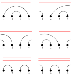
Figure 1: The six link patterns configurations for $L=4$ sites on a cylinder and two circles without sites (noncontractible loops). The open arches and circles meet behind the cylinder.

With a few exceptions, the generators $e_{k}$ act on the configurations of a given copy in the standard way MAR .

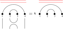
Figure 2: The action of the $e_{2}$ generator acting on the bond between the sites 2 and 3 which are not the end-points of an arch of the size of the system. $L=4$, $n=2$ in the figure.

In Fig. 2 we show the action of $e_{2}$ on one of the configurations shown in Fig. 1. The factor $x$ appears due to a contractible loop. The exceptions occur if on the copy $n$ one considers a configuration having an arch of the size $L$ of the system and if the generators acts on the bond between the two ends of the arch (see Fig. 3). The action of $e_{2}$ on the third configuration in Fig. 1 produces a new circle and therefore gives a configuration in the copy $n=3$.

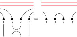
Figure 3: The action of the $e_{2}$ generator acting the bond between the sites 2 and 3 which are the end of an arch of the size of the system $L=4$. A new circle is created on the cylinder and one moves from the copy $n=2$ to the copy $n=3$.

What we have seen in this example is a general phenomenon. If a generator acts on a bond connecting two sites which are the end-points of an arch of length $L$ of the copy $n$, one obtains a configuration belonging to the copy $n+1$.

In order to get a finite-dimensional representation of the algebra, one has to take a decision. The simplest one is to identify the copy $N$ with the copy $N-1$. This possibility is illustrated in Fig. 4 for the case $N=3$ and $L=4$.

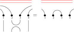
Figure 4: One takes $N=3$. The action of the generator $e_{2}$ described in Fig. 3 is changed depending of the quotient one chooses. In the figure one shows the choice of the quotient of Eq. (5). One doesn’t change the copy which stays $n=2$.

It is easy to check that one obtains in this way not a representation of the quotient (2) but of a different quotient:

$$(AB)^{N}A=(AB)^{N-1}A$$ (5)

Representations of the quotient (5) might be interesting in their own right but we didn’t study them here.

In order to obtain representations of the quotient (2) we have to identify the copy $N$ not with the copy $N-1$ but with the copy $n=0$ (no noncontractible loops). See Fig. 5 for $N=3$ and $L=4$. By adding circles without sites this representation is also a representation of the cyclic group $Z_{N}$. One can show GL that this representation is reducible. It splits into $N$ representations defined by the quotients (4) with $\alpha=\exp(i2\pi r/N)$.

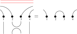
Figure 5: Same as in Fig. 4 choosing the quotient given by Eq. (2). From the copy $n=2$ one moves to the copy $n=0$ in order to get a representation with the symmetry $Z_{3}$.

In what follows we consider the application of cyclic representations to stochastic processes ALR taking $x=1$. The Hamiltonian

$$H=\sum_{k=1}^{L}(1-e_{k}),$$ (6)

gives the time evolution of the probability distribution function defined in the configuration space of the $N$ copies of link patterns each containing ${L}\choose{L/2}$ configurations. A detailed discussion of the spectra of $H$ will be presented elsewhere APR . For the remaining of this Letter we consider only even values of $L$.

We first recall the known case $N=1$. We use the spin representation of the $PTL_{L}(1)$ LEV ; MSA :

$$e_{k} = \sigma_{k}^{+}\sigma_{k+1}^{-}+\sigma_{k}^{-}\sigma_{k+1}^{+}+\frac{1}{4}(1-\sigma_{k}^{z}\sigma_{k+1}^{z})+i\frac{\sqrt{3}}{4}(\sigma_{k+1}^{z}-\sigma_{k}^{z}),\quad k=1,2,\ldots,L-1,$$

$$e_{L} = e^{i\frac{2\pi}{3}}\sigma_{L}^{+}\sigma_{1}^{-}+e^{-i\frac{2\pi}{3}}\sigma_{L}^{-}\sigma_{1}^{+}+\frac{1}{4}(1-\sigma_{L}^{z}\sigma_{1}^{z})+i\frac{\sqrt{3}}{4}(\sigma_{1}^{z}-\sigma_{L}^{z}).$$ (7)

In the scaling limit, the scaling dimensions $\{x\}$ are obtained from the leading behavior of the energy-gap amplitudes $E=2\pi v_{s}x/L$, where $v_{s}=3\sqrt{3}/2$ is the sound velocity. The spectrum of $H$ in the link representation is contained in the $S^{z}=\sum_{k=1}^{L}\sigma^{z}_{k}=0$ sector and is known. The scaling dimensions associated to the eigenstates with momenta $P=2\pi p/L$ (mod. $\pi$) ($p=0,\pm 1,\pm 2,\ldots$), are AR1 ; SAL

$$x=3/4(1/3+s)^{2}-1/12+m+m^{\prime},\quad p=m-m^{\prime}.$$ (8)

where $s,m,m^{\prime}=0,\pm 1,\pm 2,\ldots$.

The lowest excitation is obtained if one takes $s=-1,m=m^{\prime}=0$

$$x^{0}_{0}(1)=1/4=0.25,\quad p=0.$$ (9)

The explanation of the notation $x^{0}_{0}(1)$ will be given in few lines.

If $N\neq 1$, the states are separated not only by the momenta but also by the $Z_{N}$ representation $\exp(i2\pi r/N)$ to which they belong ($r=0,1,2,\ldots,N-1$). The $r=0$ states for example, are obtained by taking the sum of the same link configuration in all the $N$ copies. We will denote by $x^{r}_{p}(i)$ ($i=1,2,\ldots$) the scaling dimensions associated to the $i$-th lowest energy in the sector of momentum $P=2\pi p/L$ (mod $\pi$) and $r$ representation of $Z_{N}$. In what follows we present some results for the case $N=3$.

Although it is known DPR that the system is integrable but the calculations are tedious, we have studied the finite-size scaling spectra numerically using up to $L=30$ sites. We separate the vector space into disjoint sectors labelled by the momentum $P$ and the index $r$ of the representation $Z_{N}$. The lowest energy in each sector is calculated by the power method. The ground state of $H$ which corresponds to the stationary state of the stochastic process, corresponds to the eigenvalue zero. The eigenfunction is in the $p=0,r=0$ sector and shows no new combinatorial properties beyond those known from the $N=1$ case ZZZ . One relevant result is that the entire spectra related to the scaling dimensions $\{x^{0}_{p}(i)\}$ coincide with the known spectra of the $N=1$ representation. In order to show the precision of our procedure, we have estimated the scaling dimension (9) just from the energy gap for a $L=30$ lattice (no extrapolations using different sizes!) and got 0.24976220.

Taking $N=3$ we looked at the spectra in the $r=1$, and $p=0$ sectors and got a surprise. The extrapolantsVBS for the two first excited levels gave the following complex values:

$$x^{1}_{0}(1)=0.03905+0.08753\;i,\quad x_{0}^{1}(2)=0.14908-0.11806\;i.$$ (10)

In order to check if these results have anything to do with conformal invariant spectra, we looked at the $r=1,P=2\pi/L$ (mod. $\pi$) spectrum. If the finite-size scaling limit of the spectra are given by Virasoro representations with a complex highest weight, one should expect $x^{1}_{1}(i)=x^{1}_{0}(i)+1$ ($i=1,2$). This is indeed the case since we get:

$$x^{1}_{1}(1)=1.0391+0.08755\;i,\quad x_{1}^{1}(2)=1.149-0.11806\;i.$$ (11)

In order to illustrate the precision of the estimates of the scaling dimensions, in table 1 and 2 we give their measured values for different lattice sizes. One can see that the data converge very nicely. In the $r=2$ sector one obtains the complex conjugate values of (10) and (11): $x^{2}_{p}=(x^{1}_{p})^{{\dagger}}$. The very existence of Virasoro representations is a remarkable fact since the transitions from one copy to another is a highly nonlocal operation.

Table 1: Numerical estimates for the lowest two scaling dimensions appearing in the sector $r=1$ and momentum $0$ (mod $\pi$). In the last line of the table we show the results obtained by the van den Broeck and Swartz extrapolants (VBS). The complex conjugated dimensions appear in the sector $r=2$

$L$	$x_{0}^{1}(1)$	$x_{0}^{1}(2)$
6	$0.0411337612+0.0893222227\;i$	$0.1522015017-0.1522015017\;i$
10	$0.0398186156+0.0883428114\;i$	$0.1501651591-0.1171087213\;i$
14	$0.0394510154+0.0880912156\;i$	$0.1496233621-0.1175177089\;i$
18	$0.0392969971+0.0879921416\;i$	$0.1494051829-0.1177070065\;i$
22	$0.0392178087+0.0879436454\;i$	$0.1492965628-0.1178110010\;i$
26	$0.0391716570+0.0879165117\;i$	$0.1492349425-0.1178746350\;i$
30	$0.0391423702+0.0878998853\;i$	$0.1491967343-0.1179165804\;i$
$\infty$	$0.039050+0.087853\;i$	$0.149085-0.11806\;i$

Table 2: Numerical values of the lowest two scaling dimensions appearing in the sector $r=1$ and momentum $2\pi/L$ (mod $\pi$) (the complex conjugated dimensions appear in the sectors with $r=2$ and momentum $2\pi/L$ (mod $\pi$). In the last line of the table we show the results obtained by the VBS extrapolants.

$L$	$x_{1}^{1}(1)$	$x_{1}^{1}(2)$
6	$0.8954988326+0.0427352699\;i$	$0.9485861617-0.0543306613\;i$
10	$0.9856155271+0.0697674849\;i$	$1.0727332613-0.0917528656\;i$
14	$1.0114751102+0.0781595719\;i$	$1.1092111061-0.1038306091\;i$
18	$1.0222671807+0.0818051754\;i$	$1.1246236272-0.1091468356\;i$
22	$1.0277701176+0.0837133906\;i$	$1.1325471271-0.1119468246\;i$
26	$1.0309499010+0.0848374121\;i$	$1.1371534904-0.1136018590\;i$
30	$1.0329516135+0.0855557589\;i$	$1.1400672494-0.1146618390\;i$
$\infty$	$1.0391+0.0878\;i$	$1.149-0.11806\;i$

Notice that the scaling dimensions (10) have a smaller real part than the value (9). This observation has physical consequences. If we consider a local observable, using the mappings of the link patterns into Dyck paths, charge particles or particles-vacancies configurations ALR , for large systems, the approach to the stationary state will be oscillatory. As far as we know, it is the first time that such a phenomenon can be observed since normally the imaginary part of the energy levels decreases faster with $L$ than the real part. There are obviously consequences for the correlation functions too. We should stress that the stochastic process with the evolution operator (6) takes place in the $N$${L}\choose{L/2}$ dimensional vector space which is a representation of $Z_{N}$ and not in the independent copies (4) with $\alpha=\exp(i\pi r/N)$. The spectra are related but one has to have in mind that in a stochastic model the wavefunctions must have real nonnegative coefficients and that the various sectors are mixed.

We would like to mention that we have also looked at the variation of the lowest excited states with $N$ keeping $r=1$. The data for the second level with momentum zero (mod $\pi$) are shown in Fig. 6. One sees that increasing $N$, the real part approaches the value (9) and that the imaginary part gets smaller and smaller. This is not to say that this scaling dimension can’t be found for another value of $r$ but the consequence of the data shown in Fig. 6 is that in the large $N$ limit, the scaling dimension 1/4 will be found at least 3 times ($r=0,1$, and 2). We have not looked at the possible existence of Jordan cells in the spectrum MDA .

In APR we will give the partition function for each sector $r$ and for any parameter $x$ of the definition of the algebra LEV . The case $x=0$ is especially interesting since in this case, the Hamiltonian is related to the transfer matrix of a classical system of $N$ colored interacting polymers on a cylinder generalizing the known case $N=1$ MPR .

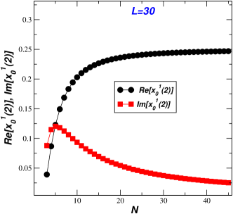
Figure 6: Real part (black) and imaginary part (red) of the estimated value of the scaling dimension $x_{0}^{1}(2)$, as a function of $N$ for the lattice size $L=30$.

I Acknowledgements

We would like to thank Alexi Morin-Duchesne, Paul Pearce, Pavel Pyatov, Hubert Saleur and Paul Martin for discussions. VR is grateful to Jan de Gier for the invitation at the Melbourne University where part of this research was done. This work was supported in part by the Australian Research Council (Australia), FAPESP and CNPq (Brazilian Agencies).

References

- (1) D. Levy, Phys. Rev. Lett. 67 (1991) 1971
- (2) F. C. Alcaraz, U. Grimm and V. Rittenberg, Nucl. Phys. B316 (1989) 735
- (3) P. Martin and H. Saleur, Comm. Math. Phys. 158 (1993) 155, Lett. Math. Phys., 30 (1994) 189
- (4) P. A. Pearce, J. Rasmussen and S. P. Villani, J. Stat. Mech. (2010) P02010
- (5) A. M. Gainutdinov, J. L. Jacobsen, N. Read, H. Saleur and R Vasseur, J. Phys. A 46 (2013) 494012 and references therein
- (6) F. C. Alcaraz and V. Rittenberg, J. Stat. Mech. (2013) P09010
- (7) P. Martin, Potts models and related problems in statistical mechanics, World Scientific (1990)
- (8) J. J. Graham and G. Lehrer, Enseign. Math. (1998)44 173, composition. Math. 133 (2002) 172, Ann. Sci. Ecole Norm. Sup. 36 (2003) 479
- (9) F. C. Alcaraz, P. Pyatov and V. Rittenberg, to be published
- (10) A. Morin-Duchesne and Y. Saint-Aubin, J. Phys. A 46 (2013) 285207
- (11) F. C. Alcaraz, M. Baake, U. Grimm and V. Rittenberg, J. Phys. A: Math. Gen. 22 (1989) L5
- (12) N. Read and H. Saleur, Nucl. Phys. B 613 (2001) 409
- (13) A. Morin-Duchesne, P. Pearce and J. Rasmussen, private communication
- (14) J. de Gier, Lecture Notes in Physics 775 (2009), ed. A. J. Guttmann, Ch. 13 (Berlin: Springer)
- (15) J. M. Van den Broeck and L. W. Schwartz, SIAM J Math. Anal. 10 (1979) 658
- (16) A. Morin-Duchesne and Y. Saint-Aubin, J.Phys. A 46 (2013) 494013