Comparison of Multigrid Algorithms for High-order Continuous Finite Element Discretizations

Abstract

We present a comparison of different multigrid approaches for the solution of systems arising from high-order continuous finite element discretizations of elliptic partial differential equations on complex geometries. We consider the pointwise Jacobi, the Chebyshev-accelerated Jacobi and the symmetric successive over-relaxation (SSOR) smoothers, as well as elementwise block Jacobi smoothing. Three approaches for the multigrid hierarchy are compared: (1) high-order $h$-multigrid, which uses high-order interpolation and restriction between geometrically coarsened meshes; (2) $p$-multigrid, in which the polynomial order is reduced while the mesh remains unchanged, and the interpolation and restriction incorporate the different-order basis functions; and (3), a first-order approximation multigrid preconditioner constructed using the nodes of the high-order discretization. This latter approach is often combined with algebraic multigrid for the low-order operator and is attractive for high-order discretizations on unstructured meshes, where geometric coarsening is difficult. Based on a simple performance model, we compare the computational cost of the different approaches. Using scalar test problems in two and three dimensions with constant and varying coefficients, we compare the performance of the different multigrid approaches for polynomial orders up to 16. Overall, both $h$- and $p$-multigrid work well; the first-order approximation is less efficient. For constant coefficients, all smoothers work well. For variable coefficients, Chebyshev and SSOR smoothing outperform Jacobi smoothing. While all of the tested methods converge in a mesh-independent number of iterations, none of them behaves completely independent of the polynomial order. When multigrid is used as a preconditioner in a Krylov method, the iteration number decreases significantly compared to using multigrid as a solver.

1 Introduction

This paper presents a comparison of geometric multigrid methods for the solution of systems arising from high-order (we target polynomial orders up to 16) continuous finite element discretizations of elliptic partial differential equations. Our particular interest is to compare the efficiency of different multigrid methods for elliptic problems with varying coefficients on complex geometries. High-order spatial discretizations for these problems can have significant advantages over low-order methods since they reduce the problem size for given accuracy, and allow for better performance on modern hardware. The main challenges in high-order discretizations are that matrices are denser compared to low-order methods, and that they lose structural properties such as the M-matrix property, which often allows to prove convergence of iterative solvers.

As illustrated in Figure 1, there are several possibilities for constructing a multigrid hierarchy for high-order discretizations: (1) high-order geometric $h$-multigrid, where the mesh is coarsened geometrically and high-order interpolation and prolongation operators are used; (2) $p$-multigrid, in which the problem is coarsened by reducing the polynomial order, and the interpolation and prolongation take into account the different order basis functions; and (3) a first-order approximation as preconditioner, constructed from the nodes of the high-order discretization. For the polynomial orders $1\leq p\leq 16$, we compare these multigrid approaches, combined with different smoothers. We also compare the use of multigrid as a solver as well as a preconditioner in a Krylov subspace method. While we use moderate size model problems (up to about $2$ million unknowns in 3D), we also discuss our findings with regard to parallel implementations on high performance computing platforms. We also discuss parallelization aspects relevant for implementations on shared or distributed memory architectures. For instance, the implementation of Gauss-Seidel smoothers can be challenging in parallel AdamsBrezinaHuEtAl03 ; BakerFalgoutKolevEtAl11 ; for this reason, we include a Chebyshev-accelerated Jacobi smoother in our comparisons. This Chebyshev smoother is easy to implement in parallel, and often is as effective a smoother as Gauss-Seidel.

We use high-order discretizations based on Legende-Gauss-Lobotto (LGL) nodal basis functions on quadrilateral or hexahedral meshes. Tensorized basis functions allow for a fast, matrix-free application of element matrices. This is particularly important for high polynomial degrees in three dimensions, as element matrices can become large. For instance, for a three-dimensional hexahedral mesh and finite element discretizations with polynomial degree $p$, the dense element matrices are of size $(p+1)^{3}\times(p+1)^{3}$. Thus, for $p=8$, this amounts to more than half a million entries per element. For tensorized nodal basis functions on hexahedral meshes, the application of elemental matrices to vectors can be implemented efficiently by exploiting the tensor structure of the basis functions, as is common for spectral elements  DevilleFischerMund02 .

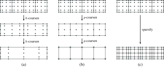
Figure 1: Illustration of different multigrid hierarchies for high-order finite element discretizations: (a) high-order $h$-multigrid, (b) $p$-multigrid and (c) low-order approximation preconditioner based on the nodes of the high-order discretization .

Related work: Multigrid for high-order/spectral finite elements has been studied as early as in the 1980s. In RonquistPatera87 , the authors observe that point smoothers such as the simple Jacobi method result in resolution-independent convergence rates for high-order elements on simple one and two-dimensional geometries. Initial theoretical evidence for this behavior is given in MadayMunoz88 , where multigrid convergence is studied for one-dimensional spectral methods and spectral element problems. The use of $p$-multigrid is rather common in the context of high-order discontinuous Galerkin discretizations FidkowskiOliverLuEtAl05 ; HelenbrookAtkins06 , but $p$-multigrid has also been used for continuous finite element discretizations  HelenbrookMavriplisAtkins03 . A popular strategy for high-order discretizations on unstructured meshes, for which geometric mesh coarsening is challenging, is to assemble a low-order approximation of the high-order system and use an algebraic multigrid method to invert the low-order (and thus much sparser) operator Brown10 ; Kim07 ; DevilleMund90 ; Olson07 ; CanutoGervasioQuarteroni10 . In HeysManteuffelMcCormickEtAl05 , this approach is compared with the direct application of algebraic multigrid to the high-order operator and the authors find that one of the main difficulties is the assembly of the high-order matrices required by algebraic multigrid methods.

Contributions: There has been a lot of work on high-order discretization methods and on the efficient application of the resulting operators. However, efficient solvers for such discretization schemes have received much less attention. In particular, theoretical and experimental studies are scattered regarding the actual performance (say the number of v-cycles or matrix-vector products to solve a system) of the different schemes under different scenarios. A systematic analysis of such performance is not available. In this paper, we address this gap in the existing literature. In particular we (1) consider high-order continuous Galerkin discretizations up to 16th order, (2) examine three different multigrid hierarchies ($h$, $p$, and first-order), (3) examine several different smoothers: Jacobi, polynomial, SSOR, and block Jacobi, (4) consider different settings (constant, mildly variable, and highly variable) of coefficients and (5) consider problems in 2D and 3D. To our knowledge, this is the first study of this kind. Our results demonstrate significant variability in the performance of the different schemes for higher-order elements, highlighting the need for further research on the smoothers. Although the overall runtime will depend on several factors—including the implementation and the target architecture—in this work we limit ourselves to characterizing performance as the number of fine-grid matrix-vector products needed for convergence. This is the most dominant cost and is also independent of the implementaion and architecture, allowing for easier interpretation and systematic comparison with other approaches. Finally, we provide an easily extendable Matlab implementation, which allows a systematic comparison of the different methods in the same framework.

Limitations: While this work is partly driven by our interest in scalable parallel simulations on nonconforming meshes derived from adaptive octrees (e.g.,SundarBirosBursteddeEtAl12 ), for the comparisons presented in this paper we restrict ourselves to moderate size problems on conforming meshes. We do not fully address time-to-solution, as we do not use a high-performance implementation. However, recent results using a scalable parallel implementation indicate that many of our observations generalize to non-conforming meshes and that the methods are scalable to large parallel computers GholaminejadMalhotraSundarEtAl14 . While we experiment with problems with strongly varying coefficients, we do not study problems with discontinuous or anisotropic coefficients, nor consider ill-shaped elements.

Organization of this paper: In §2 we describe the test problem, as well as discretization approach for the different multigrid schemes. In §3, we describe in detail the different multilevel approaches for solving the resulting high-order systems. In §4, we present a comprehensive comparison of different approaches using test problems in 2D and 3D. Finally, in §5 we draw conclusions and discuss our findings.

2 Problem statement and preliminaries

We wish to solve the Poisson problem with homogeneous Dirichlet boundary conditions on an open bounded domain $\Omega\subset\mathbb{R}^{d}$ ($d=2$ or $d=3$) with boundary $\partial\Omega$, i.e., we search the solution $u(\boldsymbol{x})$ of:

$$-\nabla\cdot\left(\mu(\boldsymbol{x})\nabla u(\boldsymbol{x})\right) =f(\boldsymbol{x})\quad \text{ for }\boldsymbol{x}\in\Omega,$$ (1)

$$\quad u(\boldsymbol{x}) =0\quad \text{ for }\boldsymbol{x}\in\partial\Omega.$$

Here, $\mu(\boldsymbol{x})\geq\mu_{0}>0$ is a spatially varying coefficient that is bounded away from zero, and $f(x)$ is a given right hand side. We discretize (1) using finite elements with basis functions of polynomial order $p$ and solve the resulting discrete system using different multigrid variants. Next, in §2.1 and §2.2, we discuss the Galerkin approximation to (1) and the setup of the inter-grid transfer operators to establish a multilevel hierarchy. In §2.3, we discuss details of the meshes and implementation used for our comparisons.

2.1 Galerkin approximation

Given a bounded, symmetric bilinear form $a(u,v)$ that is coercive on $H_{0}^{1}(\Omega)$, and $f\in L^{2}(\Omega)$, we want to find $u\in H_{0}^{1}(\Omega)$ such that $u$ satisfies

$$a(u,v)=(f,v)_{L^{2}(\Omega)},\ \ \ \forall v\in H_{0}^{1}(\Omega),$$ (2)

where $(f,v)_{L^{2}(\Omega)}=\int_{\Omega}fv\,dx$ and $H_{0}^{1}(\Omega)\subset L^{2}(\Omega)$ denotes the subspace of functions with square integrable derivatives that vanish on the boundary. This problem is known to have a unique solution $u^{*}$ BrennerScott94 . We now derive discrete equations whose solutions approximate the solution of (2). First, we define a sequence of $m$ nested conforming finite-dimensional spaces, $V_{1}\subset V_{2}\subset\cdots\subset V_{m}\subset H_{0}^{1}(\Omega)$. Here, $V_{k}$ is the finite element space that corresponds to a finite element mesh at a specified polynomial order, and $V_{k-1}$ corresponds to the next coarser problem, as illustrated in Figure 1-(a,b) for different coarsenings. Then, the discretized problem on $V_{k}$ is to find $u_{k}\in V_{k}$ such that

$$a(u_{k},v_{k})=(f,v_{k})_{L^{2}(\Omega)},\ \ \ \forall v_{k}\in V_{k}.$$ (3)

This problem has a unique solution, and the sequence $\{u_{k}\}$ converges to $u^{*}$ BrennerScott94 . The $L^{2}$-projection of the linear operator corresponding to the bilinear form $a(\cdot\,,\cdot)$ onto $V_{k}$ is defined as the linear operator $A_{k}:V_{k}\rightarrow V_{k}$ such that

$$(A_{k}v_{k},w_{k})_{L^{2}(\Omega)}=a(v_{k},w_{k}),\ \ \ \forall v_{k},w_{k}\in V_{k}.$$ (4)

The operator $A_{k}$ is self-adjoint with respect to the $L^{2}$-inner product and positive definite. Let $\{\phi_{1}^{k},\phi_{2}^{k},\ldots,\phi_{N_{k}}^{k}\}$ be a basis for $V_{k}$ and denote by $\mathbf{A_{k}}$ the representation of $A_{k}$ in that basis. Then, (4) becomes the linear matrix equation for the coefficient vector $\mathbf{u}_{k}\in\mathbb{R}^{N_{k}}$

$$\mathbf{A}_{k}\mathbf{u}_{k}=\mathbf{f}_{k},$$ (5)

where, for $i,j=1,2,\ldots,N_{k}$, the components of $\mathbf{A}_{k}$, $\mathbf{u}_{k}$ and $\mathbf{f}_{k}$ are given by

$$(\mathbf{A}_{k})_{ij}= a(\phi_{i}^{k},\phi_{j}^{k}),$$

$$(\mathbf{f}_{k})_{j}= (f,\phi_{j}^{k})_{L^{2}(\Omega)},$$

$$(\mathbf{M}_{k})_{ij}= (\phi_{i}^{k},\phi_{j}^{k})_{L^{2}(\Omega)},$$

where the integrals on the right hand sides are often approximated using numerical quadrature. Here, $\mathbf{M}_{k}$ is the mass matrix, which appears in the approximation of the $L^{2}$-inner product in $V_{k}$ since $(u_{k},v_{k})_{L^{2}(\Omega)}=\mathbf{u}_{k}^{T}\mathbf{M}_{k}\mathbf{v}_{k}$ for all $u_{k},v_{k}\in V_{k}$ with corresponding coefficient vectors $\mathbf{u}_{k},\mathbf{v}_{k}\in\mathbb{R}^{N_{k}}$.

2.2 Restriction and prolongation

Since the coarse-grid space is a subspace of the fine-grid space, any coarse-grid function $v_{k-1}$ can be expanded in terms of the fine-grid basis functions,

$$v_{k-1}=\sum_{i=1}^{N_{k-1}}\mathbf{v}_{i,k-1}\phi_{i}^{k-1}=\sum_{j=1}^{N_{k}}\mathbf{v}_{j,k}\phi_{j}^{k},$$ (6)

where, $\mathbf{v}_{i,k}$ and $\mathbf{v}_{i,k-1}$ are the coefficients in the basis expansion for $v_{k-1}$ on the fine and coarse grids, respectively.

The application of the prolongation operator can be represented as a matrix-vector product with the input vector as the coarse grid nodal values and the output as the fine grid nodal values SampathBiros10 . The matrix entries of this operator are thus the coarse grid shape functions evaluated at the fine-grid vertices, $p_{i}$, i.e.,

$$\mathbf{P}_{\!ij}=\phi_{j}^{k-1}(p_{i})\quad\text{ for }1\leq i\leq N_{k},1\leq j\leq N_{k-1}.$$ (7)

This gives rise to two different operators depending on whether the coarse grid is obtained via $h$-coarsening or whether it is obtained via $p$-coarsening; see Figure 1 for an illustration of the two cases. The restriction operator is the adjoint of the prolongation operator with respect to the mass-weighted inner products. This only requires the application of the transpose of the prolongation operator to vectors.

2.3 Meshing and implementation

For the numerical comparisons in this work we consider domains that are the image of a square or a cube under a diffeomorphism, i.e., a smooth mapping from the reference domain $S\coloneqq[0,1]^{d}$ to the physical domain $\Omega$. Hexahedral finite element meshes and tensorized nodal basis function based on Legende-Gauss-Lobotto (LGL) points are used. We use isoparametric elements to approximate the geometry of $\Omega$, i.e., on each element the geometry diffeomorphism is approximated using the same basis functions as the finite element approximation. The Jacobians for this transformation are computed at every quadrature point, and Gauss quadrature is used to numerically approximate integrals. We assume that the coefficient $\mu$ is a given function, which, at each level, can be evaluated at the respective quadrature points. We restrict our comparisons to uniformly refined conforming meshes and our implementation, written in Matlab, is publicly available. It allows comparisons of different smoothing and coarsening methods for high-order discretized problems in two and three dimensions, and can easily be modified or extended. It does not support distributed memory parallelism, and is restricted to conforming meshes that can be mapped to a square (in 2D) or a cube (in 3D). While, in practice, matrix assembly for high-order discretizations is discouraged, we use sparse assembled operators in this prototype implementation.

Note that for hexahedral elements in combination with a tensorial finite element basis, the effect of matrix-free operations for higher-order elements can be quite significant in terms of floating point operations, memory requirements, and actual run time:

• Memory requirements for assembled matrices: For an order $p$, assembled element matrices are dense and of the size $(p+1)^{3}\times(p+1)^{3}$. For $p=9$, for instance, $(p+1)^{3}=1000$ and thus each element contributes $10^{6}$ entries to the assembled stiffness matrix, and each row in the matrix contains, on average, several 1000 nonzero entries. Thus, for high orders, memory becomes a significant issue.

• Floating point operations for matrix-free versus assembled MatVec: For hexahedral elements, the operation count for a tensorized matrix-free matvec is $\mathcal{O}(p^{4})$ as opposed to $\mathcal{O}(p^{6})$ for a fully assembled matrix orszag80 ; DevilleFischerMund02 .

Detailed theoretical and experimental arguments in favor of matrix-free approaches, especially for high-order discretizations can be found in DevilleFischerMund02 ; BursteddeGhattasGurnisEtAl08 ; MayBrownLePourhiet14

3 Multigrid approaches for high-order finite element discretizations

In this section, we summarize different multigrid approaches for high-order/spectral finite element discretizations, which can either be used as a solver or can serve as a preconditioner within a Krylov method. We summarize different approaches for the construction of multilevel hierarchies in §3.1 and discuss smoothers in §3.2.

3.1 Hierarchy construction, restriction and prolongation operators

There are several possibilities to build a multilevel hierarchy for high-order discretized problems; see Figure 1. One option is the construction of a geometric mesh hierarchy while keeping the polynomial order unchanged; we refer to this approach as high-order $h$-multigrid. An alternative is to construct coarse problems by reducing the polynomial degree of the finite element basis functions, possibly followed by standard geometric multigrid; this is commonly referred to as $p$-multigrid. For unstructured high-order element discretizations, where geometric coarsening is challenging, using an algebraic multigrid hierarchy of a low-order approximation to the high-order operator as a preconditioner has proven efficient. Some details of these different approaches are summarized next.

3.1.1 $h$-multigrid

A straightforward extension of low-order to high-order geometric multigrid is to use the high-order discretization of the operator for the residual computation on each multigrid level, combined with high-order restriction and prolongation operators (see §2.2). For hexahedral (or quadrilateral) meshes, the required high-order residual computations and the application of the interpolation and restriction operators can often be accelerated using elementwise computations and tensorized finite element basis functions, as is common in spectral element methods DevilleFischerMund02 .

3.1.2 $p$-multigrid

In the $p$-multigrid approach, a multigrid hierarchy is obtained by reducing the polynomial order of the element basis functions. Starting from an order-$p$ polynomial basis (for simplicity, we assume here that $p$ is a power of 2), the coarser grids correspond to polynomials of order $p/2,p/4,\ldots,1$, followed by geometric coarsening of the $p=1$ grid (i.e., standard low-order geometric multigrid). As for high-order $h$-multigrid, devising smoothers can be a challenge for $p$-multigrid. Moreover, one often finds dependence of the convergence factor on the order of the polynomial basis MadayMunoz89 .

3.1.3 Preconditioning by lower-order operator

In this defect correction approach (see TrottenbergOosterleeSchuller01 ; Hackbusch85 ), the high-order residual is iteratively corrected using a low-order operator, obtained by overlaying the high-order nodes with a low-order (typically linear) finite element mesh. While the resulting low-order operator has the same number of unknowns as the high-order operator, it is much sparser and can, thus, be assembled efficiently and provided as input to an algebraic multigrid method, which computes a grid hierarchy through algebraic point aggregation. This construction of a low-order preconditioner based on the nodes of the high-order discretization is used, for instance in Brown10 ; Kim07 ; DevilleMund90 ; HeysManteuffelMcCormickEtAl05 . Due to the black-box nature of algebraic multigrid, it is particularly attractive for high-order discretizations on unstructured meshes. Note that even if the mesh is structured, it is not straightforward to use low-order geometric multigrid since the nodes—inherited from the high-order discretization—are not evenly spaced (see Figure 1).

3.2 Smoothers

In our numerical comparisons, we focus on point smoothers but we also compare with results obtained with an elementwise block-Jacobi smoother. In this section, we summarize different smoothers and numerically study their behavior for high-order discretizations. Note that, multigrid smoothers must target the reduction of the error components in the upper half of the spectrum.

3.2.1 Point smoothers

We compare the Jacobi and the symmetric successive over relaxation (SSOR) smoothers, as well as a Chebyshev-accelerated Jacobi smoother Brandt77 . All of these smoothers require the diagonal of the system matrix; if this matrix is not assembled (i.e., in a matrix-free approach), these diagonal entries must be computed in a setup step; for high-order discretizations on deformed meshes, this can be a significant computation. Note that the parallelization of Gauss-Seidel smoothers (such as SSOR) requires coloring of unknowns in parallel, and, compared to Jacobi smoothing, more complex communication in a distributed memory implementation. The Chebyshev-accelerated Jacobi method is an alternative to SSOR; it can significantly improve over Jacobi smoothing, while being as simple to implement AdamsBrezinaHuEtAl03 . The acceleration of Jacobi smoothing with Chebyshev polynomials requires knowledge of the maximum eigenvalue of the system matrix, usually estimated during setup with an iterative solver.

3.2.2 Comparison of point smoothers

In Figures 2 and 3, we compare the efficiency of these point smoothers for different polynomial orders and constant and varying coefficients. For that purpose, we compute the eigenvectors of the system matrix, choose a zero right hand side and an initialization that has all unit coefficients in the basis given by these eigenvectors. For the polynomial orders $p=1,4,16$, we compare the performance of point smoothers with and without a 2-level v-cycle with exact coarse solve. The coarse grid for all polynomial orders is obtained using $h$-coarsening. We depict the coefficients after six smoothing steps in the left column, and the results obtained for a two-grid method with three pre- and three post-smoothing steps (and thus overall six smoothing steps on the finest grid) in the right column. The SSOR smoother uses a lexicographic ordering of the unknowns, and we employ two pre- and one post-smoothing steps, which again amounts to overall six smoothing steps on the finest grid. The damping factors for Jacobi and SSOR smoothing are $\omega=2/3$ and $\omega=1$, respectively. The Chebyshev smoother targets the part of the spectrum given by $[\lambda_{\text{max}}/4,\lambda_{\text{max}}]$, where $\lambda_{\text{max}}$ is the maximum eigenvalue of the system matrix, which is estimated using 10 iterations of the Arnoldi algorithm.

The results for the constant coefficient Laplacian operator on the unit square (see Figure 2) show that all point smoothers decrease the error components in the upper half of the spectrum; however, the decrease is smaller for high-order elements. Observe that compared to Jacobi smoothing, Chebyshev accelerated Jacobi smoothing dampens a larger part of the spectrum. Both, the Chebyshev and SSOR methods outperform Jacobi smoothing, in particular for higher orders. Combining the smoothers with a two-grid cycle, all error components are decreased for all smoothers (and thus the resulting two-grid methods converge, see Table 1 in §4.4), but the error decreases slower for higher polynomial orders. For high polynomial orders, a two-grid iteration with SSOR smoothing results in a much better error reduction than Jacobi or Chebyshev smoothing.

In Figure 3, we study the performance of different smoothers for the test problem 2d-var, defined in §4.1. In this problem, we solve (1) with a strongly (but smoothly) varying coefficient $\mu$ on a deformed domain $\Omega$. Compared to the constant coefficient case, Jacobi smoothing performs worse, both, when used as a solver and as a smoother. Let us focus on the two-grid correction for polynomial order $p=16$ and compare with the results obtained when using multigrid as a solver, shown in Table 2. Jacobi smoothing does not lead to a converging two-grid algorithm, as several coefficients are amplified by the two-grid cycle. For Chebyshev smoothing, the multigrid v-cycle converges slowly although one or two coefficients appear amplified in the two-grid iteration. This convergence can be explained by the fact that errors can be interchanged between different eigenvectors in the v-cycle. SSOR smoothing combined with the two-grid method retains a significant error reduction rate and, as a consequence, converges quickly.

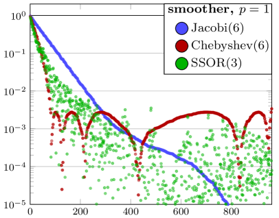
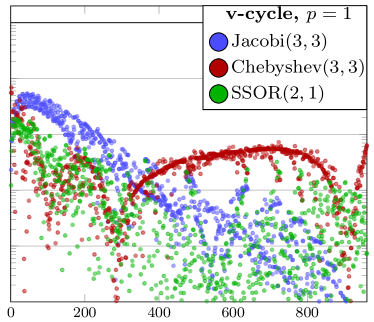
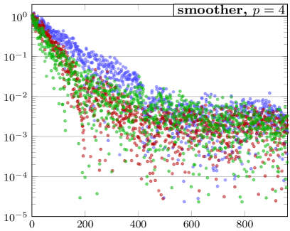
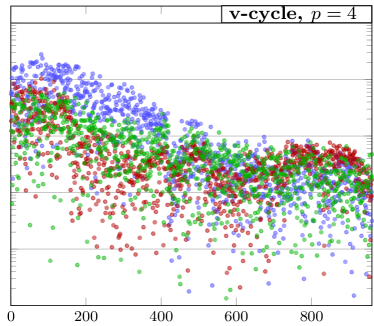
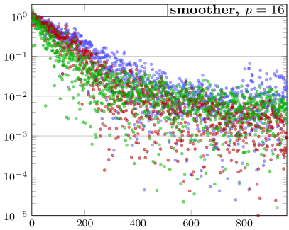
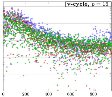
Figure 2: Error decay for different point smoothers when used as solver (left column) and when used in a single two-grid step with exact coarse grid solution (right column) for a two-dimensional, constant coefficient Laplace problem on a unit square (problem 2d-const specified in §4.1). To keep the number of unknowns the same accross all polynomial orders, meshes of $32\times 32$, $8\times 8$ and $2\times 2$ elements are used for polynomial orders $p=1$, $p=4$ and $p=16$, respectively. The horizontal axis is the index for the eigenvectors of the system matrix $\mathbf{A}_{k}$, and the vertical axis is the magnitude of the error component for each eigenvector. The eigenvectors are ordered such that the corresponding eigenvalues are ascending; thus, due to the properties of $\mathbf{A}_{k}$, the smoothness in every eigenvector decays from left to right. The system right hand side is zero and the initialization is chosen to have all unit coefficients in the eigenvector expansion. A total of six smoothing steps is used for all methods, and the coarse problem in the two-grid step is solved by a direct solver.

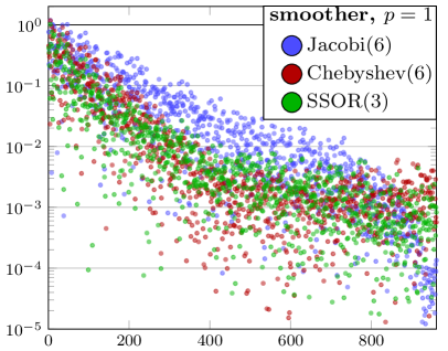
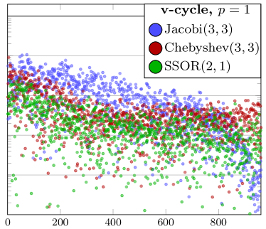
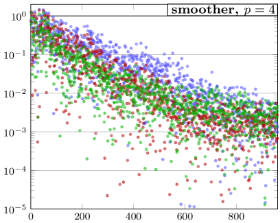
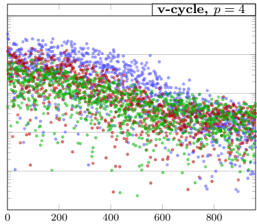
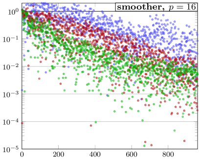
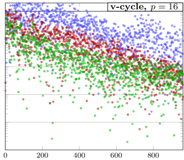
Figure 3: Shown is the same comparison as in Figure 2, but for the two-dimensional warped geometry, variable coefficient problem 2d-var specified in §4.1.

3.2.3 Block-Jacobi smoothing

An alternative smoothing approach for high-order discretizations is based on local block solves. Since for high polynomial orders many unknowns lie in the element interiors, Schwarz-type domain decomposition smoothers are promising. For instance, they are more stable for anisotropic meshes than point smoothers. A main challenge of Schwarz-type smoothers is that they require the solution of dense local systems. This is either done by using direct methods or approximations that allow for a fast iterative solution on hexahedral meshes LottesFischer05 ; FischerLottes05 . In §4, we compare the performance of point smoothers with an elementwise block Jacobi smoothing.

4 Numerical results

In this section, we present a comprehensive comparison of our algorithms for the solution of high-order discretizations of (1). After introducing our test problems in §4.1, we present a simple model for the computational cost of the different approaches in terms of matrix-vector applications in §4.2. In §4.3, we specify settings and metrics for our comparisons. The results of these comparisons are presented and discussed in §4.4.

4.1 Test problems

We compare our algorithms for the solution of (1) with constant coefficient $\mu\equiv 1$ on the unit square and the unit cube, and, with varying coefficients $\mu(\boldsymbol{x})$, on the warped two and three-dimensional domains shown in Figure 4. To be precise, we consider the following four problems:

• 2d-const: The domain $\Omega$ for the problem is the unit square, and $\mu\equiv 1$.

• 2d-var: The warped two-dimensional domain $\Omega$ is shown on the left in Figure 4, and the varying coefficient is $\mu(x,y)=1+10^{6}(\cos^{2}(2\pi x)+\cos^{2}(2\pi y))$. We also study a modification of this problem with a more oscillatory coefficient $\mu(x,y)=1+10^{6}(\cos^{2}(10\pi x)+\cos^{2}(10\pi y))$, which we refer to as 2d-var^′.

• 3d-const: For this problem, $\Omega$ is the unit cube, and we use the constant coefficient $\mu\equiv 1$.

• 3d-var: The warped three-dimensional domain $\Omega$ shown on the right of Figure 4 is used; the varying coefficient is $\mu(x,y,z)=1+10^{6}(\cos^{2}(2\pi x)+\cos^{2}(2\pi y)+\cos^{2}(2\pi z))$.

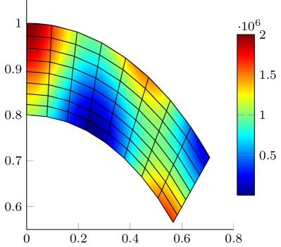
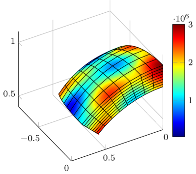
Figure 4: Two and three-dimensional warped meshes used in our numerical experiments. The color illustrates the logarithm of the coefficient field, which varies over six orders of magnitude.

4.2 Comparing the computational cost

To compare the computational cost of the different methods, we focus on the matrix-vector multiplications on the finest multigrid level, which dominate the overall computation. Denoting the number of unknowns on the finest level by $N$, the computational cost—measured in floating point operations (flops)—for a matrix-vector product is $Ng_{p}$, where $g_{p}$ is the number of flops per unknown and the subscript $p$ indicates the polynomial order used in the FEM basis. Since high-order discretizations result in less sparse operators, $g_{1}\leq g_{2}\leq\ldots$ holds. The actual value of $g_{p}$ depends strongly on the implementation. Also note that the conversion from $g_{p}$ to wall-clock time is not trivial, as wall-clock timings depend on caching, vectorization, blocking and other effects. Thus, although $g_{p}$ increases with $p$, wall-clock times might not increase as significantly. In general, high-order implementations allow more memory locality, which often results in higher performance compared to low-order methods. This discussion, however, is beyond the scope of this paper.

The dominant computational cost per iteration of the high-order multigrid approaches discussed in §3 can thus be summarized as

$$Ng_{p}(1+m(s_{\text{pre}}+s_{\text{post}})).$$ (8)

Here, we denote by $s_{\text{pre}}$ and $s_{\text{post}}$ the number of pre- and post-smoothing steps on the finest multigrid level, respectively. Moreover, $m$ denotes the number of residual computations (and thus matrix-vector computations) per smoothing step. Jacobi smoothing and Chebyshev-accelerated Jacobi require $m=1$ matrix-vector multiplication per smoothing step, while SSOR requires $m=2$ matrix-vector operations. If, in the approach discussed in §3.1.3, the sparsified linear-element residual is used in the smoother on the finest grid, the cost (8) reduces to

$$N(g_{p}+g_{1}m(s_{\text{pre}}+s_{\text{post}})).$$ (9)

However, since the overall number of iterations increases (see §4.4), this does not necessarily decrease the solution time.

If the overall number of unknowns $N$ is kept fixed and the solution is smooth, it is well known that the accuracy increases for high-order discretizations. Due to the decreased sparsity of the discretized operators, this does not automatically translate to more accuracy per computation time; see, e.g., Brown10 . However, note that many computations in, for instance, a multigrid preconditioned conjugate gradient algorithm are of complexity $\mathcal{O}(N)$ (see Algorithm 4.1) and are thus independent of $g_{p}$. Thus, the computational cost of these steps does not depend on the order of the discretization. Even if these $\mathcal{O}(N)$ steps do not dominate the computation, they contribute to making high-order discretizations favorable not only in terms of accuracy per unknown, but also in terms of accuracy per computation time.

Algorithm 4.1 Complexity of individual steps in multigrid-preconditioned CG

1:rhs and guess

2:solution

3:while not converged do

4:     $\boldsymbol{h}=A\boldsymbol{p}$ $\triangleright$ $~{}~{}\quad\quad\quad\quad\mathcal{O}(Ng_{p})$

5:     $\rho_{r}=(\rho,\boldsymbol{r})$ $\triangleright$ $~{}~{}\quad\quad\quad\quad\mathcal{O}(N)~{}~{}~{}$

6:     $\alpha=\rho_{r}/(\boldsymbol{p},\boldsymbol{h})$ $\triangleright$ $~{}~{}\quad\quad\quad\quad\mathcal{O}(N)~{}~{}~{}$

7:     $\boldsymbol{u}=\boldsymbol{u}+\alpha\boldsymbol{p}$ $\triangleright$ $~{}~{}\quad\quad\quad\quad\mathcal{O}(N)~{}~{}~{}$

8:     $\boldsymbol{r}=\boldsymbol{r}-\alpha\boldsymbol{h}$ $\triangleright$ $~{}~{}\quad\quad\quad\quad\mathcal{O}(N)~{}~{}~{}$

9:     Convergence Test

10:     $\rho=M\boldsymbol{r}$ $\triangleright$ v-cycle $\quad\mathcal{O}(Ng_{p})$

11:     $\beta=(\rho,\boldsymbol{r})/\rho_{r}$ $\triangleright$ $~{}~{}\quad\quad\quad\quad\mathcal{O}(N)~{}~{}~{}$

12:     $\boldsymbol{p}=\rho+\beta\boldsymbol{p}$ $\triangleright$ $~{}~{}\quad\quad\quad\quad\mathcal{O}(N)~{}~{}~{}$

13:end while

4.3 Setup of comparisons

We test the different multigrid schemes in two contexts: as solvers and as preconditioners in a conjugate gradient (CG) method. In tables 1–5, we report the number of multigrid v-cycles required to reduce the norm of the discrete residual by a factor of $10^{8}$, where a “-” indicates that the method did not converge within the specified maximum number of iterations. In particular, these tables report the following information:

• The first column gives the polynomial order used in the finite element discretization.

• The columns labeled MG as solver report the number of v-cycles required for convergence when multigrid is used as solver. The subcolums are:

  • Jacobi(3,3) denotes that 3 pre-smoothing and 3 post-smoothing steps of a pointwise Jacobi smoother are used on each level. We use a damping factor $\omega=2/3$ in all experiments.

  • Cheb(3,3) indicates that Chebyshev-accelerated Jacobi smoothing is used, again using 3 pre-smoothing and 3 post-smoothing steps. An estimate for the maximal eigenvalue of the linear systems on each level, as required by the Chebyshev method, is computed in a setup step using 10 Arnoldi iterations.

  • SSOR(2,1) denotes that a symmetric successive over-relaxation method is employed, with 2 pre-smoothing and 1 post-smoothing steps. Note that each SSOR iteration amounts to a forward and a backward Gauss-Seidel smoothing step, and thus requires roughly double the computational work compared to Jacobi smoothing. The SSOR smoother is based on a lexicographic ordering of the unknowns, and the damping factor is $\omega=1$.

  For the two-dimensional problems reported in Tables 1–3, we use a multigrid hierarchy with three levels corresponding to meshes with $32\times 32$, $16\times 16$ and $8\times 8$ elements. The multigrid hierarchy for the three-dimensional tests reported in Tables 4 and 5 also has three levels with $8\times 8\times 8$, $4\times 4\times 4$ and $2\times 2\times 2$ elements. Note that for each smoother we report results for $h$-multigrid (columns marked by h; see §3.1.1) as well as for $p$-multigrid (columns marked by p; see §3.1.2). For $p$-multigrid, we restrict ourselves to orders that are powers of 2. After coarsening in $p$ till $p=1$, we coarsen in $h$. For example, for the two-dimensional problems and $p=16$, we use a total of 7 grids; the first five all use meshes with $32\times 32$ elements, and $p=16,8,4,2,1$, respectively, followed by two additional coarse grids of size $16\times 16$ and $8\times 8$, and $p=1$.

• The columns labeled MG with pCG present the number of conjugate gradient iterations required for the solution, where each iteration uses one multigrid v-cycle as preconditioner. The sub-columns correspond to different smoothers, as described above.

• The columns labeled low-order MG pCG report the number of CG iterations needed to solve the high-order system, when preconditioned with the low-order operator based on the high-order nodal points (see §3.1.3). While in practice one would use algebraic multigrid to solve the linearized system approximately, in our tests we use a factorization method to solve the low-order system directly. As a consequence, the reported iteration counts are a lower bound for the iteration counts one would obtain if the low-order system was inverted approximately by algebraic multigrid.

Note that the number of smoothing steps in the different methods is chosen such that, for fixed polynomial order, the computational work is comparable. Each multigrid v-cycle requires one residual computation and overall six matrix-vector multiplications. Following the simple complexity estimates (8) and (9), this amounts to a per-iteration cost of $7Ng_{p}$ for $h$- and $p$-multigrid, and of $N(g_{1}+6g_{p})$ for the low-order multigrid preconditioner. As a consequence, the iteration numbers reported in the next section can be used to compare the efficiency of the different methods. Note that in our tests, we change the polynomial degree of the finite element functions but retain the same mesh. This results in an increasing number of unknowns as $p$ increases. Since, as illustrated in §4.4.2, we observe mesh independent convergence for fixed $p$, this does not influence the comparison.

4.4 Summary of numerical results

Next, in §4.4.1, we compare the performance of different point smoothers for the test problems presented in §4.1. Then, in §4.4.2, we illustrate that the number of iterations is independent of the mesh resolution. Finally, in §4.4.3, we study the performance of a block Jacobi smoother for discretizations with polynomial orders $p=8$ and $p=16$.

Table 1: Iteration counts for the two-dimensional unit square problem 2d-const defined in §4.1. The finest mesh has $32\times 32$ elements and the multigrid hierarchy consists of three meshes. For $p$-multigrid, the polynomial order is first reduced to $p=1$, followed by two geometric coarsenings of the mesh. For a detailed description of the different experiments reported in this table we refer to §4.3.

	MG as solver						MG with pCG						​​low-order MG​​
​​​ order	​​Jacobi(3,3)​​		​​Cheb(3,3)​​		​​SSOR(2,1)​​		​​Jacobi(3,3)​​		​​Cheb(3,3)​​		​​SSOR(2,1)​​		pCG
	$h$	$p$	$h$	$p$	$h$	$p$	$h$	$p$	$h$	$p$	$h$	$p$
1	6		5		5		5		4		4		-
2	7	7	5	6	5	5	5	5	4	4	4	4	14
3	8		6		5		6		5		4		16
4	9	8	6	6	5	5	6	5	5	5	4	4	16
5	12		8		7		7		6		5		17
6	12		9		7		7		6		5		18
7	16		12		8		8		7		6		18
8	17	14	13	10	8	7	9	8	7	6	6	5	19
16	40	33	33	27	17	14	14	12	12	11	9	8	21

4.4.1 Comparison of different multigrid/smoothing combinations

Tables 1–3 present the number of iterations obtained for various point smoothers and different polynomial orders for the two-dimensional test problems. As can be seen in Table 1, for 2d-const all solver variants converge in a relatively small number of iterations for all polynomial orders. However, the number of iterations increases with the polynomial order $p$, in particular when multigrid is used as a solver. Using multigrid as a preconditioner in the conjugate gradient method results in a reduction of overall multigrid v-cycles, in some cases even by a factor or two. Also, we observe that SSOR smoothing generally performs better than the two Jacobi-based smoothers. We find that the linear-order operator based on the high-order nodes is a good preconditioner for the high-order system. Note that if algebraic multigrid is used for the solution of the low-order approximation, the smoother on the finest level can either use the residual of the low-order or of the high-order operator. Initial tests that mimic the use of the high-order residual in the fine-grid smoother show that this has the potential to reduce the number of iterations.

Let us now contrast these observations with the results for the variable coefficient problems 2d-var and 2d-var^′ summarized in Tables 2 and 3. First, note that all variants of the solver perform reasonably for discretizations up to order $p=4$. When used as a solver, multigrid either diverges or converges slowly for orders $p>4$. Convergence is reestablished when multigrid is combined with CG. Using multigrid with SSOR smoothing as preconditioner in CG yields, for orders up to $p=8$, convergence with a factor of at least $0.1$ in each iteration. Comparing the results for 2d-var shown in Table 2 with the results for 2d-var^′ in Table 3 shows that the convergence does not degrade much for the coefficient with 5-times smaller wavelength.

Next, we turn to the results for 3d-const and 3d-var, which we report in Tables 4 and 5, respectively. For 3d-const, all variants of the solver converge. For this three-dimensional problem, the benefit of using multigrid as preconditioner rather than as solver is even more evident than in two dimensions.

Our results for 3d-var are summarized in Table 5. As for 2d-var, the performance of multigrid when used as a solver degrades for orders $p>4$. We can also observe that the low-order matrix based on the high-order node points represents a good preconditioner for the high-order system.

Table 2: Iteration counts for two-dimensional warped-geometry, varying coefficient problem 2d-var defined in §4.1. The finest mesh has $32\times 32$ elements and the multigrid hierarchy consists of three meshes. For $p$-multigrid, the polynomial order is first reduced to $p=1$, followed by two geometric coarsenings of the mesh. For a detailed description of the different experiments reported in this table we refer to §4.3.

	MG as solver						MG with pCG						​​low-order MG​​
​​​ order	​​Jacobi(3,3)​​		​​Cheb(3,3)​​		​​SSOR(2,1)​​		​​Jacobi(3,3)​​		​​Cheb(3,3)​​		​​SSOR(2,1)​​		pCG
	$h$	$p$	$h$	$p$	$h$	$p$	$h$	$p$	$h$	$p$	$h$	$p$
1	14		11		6		8		7		5		-
2	20	19	15	15	7	8	10	10	8	8	5	6	16
3	20		16		8		10		9		6		18
4	22	21	21	19	10	9	11	10	10	10	7	6	19
5	-		28		12		14		12		7		21
6	-		35		13		15		13		8		23
7	-		45		16		18		15		9		24
8	-	-	52	46	17	15	20	20	16	15	9	8	25
16	-	-	169	148	37	33	51	45	30	27	13	12	31

Table 3: Iteration counts for two-dimensional warped-geometry, varying coefficient problem 2d-var^′ defined in §4.1. This problem is identical to 2d-var (see Table 2), but the variations in the coefficient $\mu$ have a smaller wave length. The finest mesh has $32\times 32$ elements and the multigrid hierarchy consists of three meshes. For $p$-multigrid, the polynomial order is first reduced to $p=1$, followed by two geometric coarsenings of the mesh. For a detailed description of the different experiments reported in this table we refer to §4.3.

	MG as solver						MG with pCG						​​low-order MG​​
​​​ order	​​Jacobi(3,3)​​		​​Cheb(3,3)​​		​​SSOR(2,1)​​		​​Jacobi(3,3)​​		​​Cheb(3,3)​​		​​SSOR(2,1)​​		pCG
	$h$	$p$	$h$	$p$	$h$	$p$	$h$	$p$	$h$	$p$	$h$	$p$
1	14		12		8		8		8		6		-
2	19	19	15	14	7	8	10	10	8	8	6	6	19
3	20		17		8		10		9		6		22
4	261	333	21	20	10	9	15	15	11	10	7	6	26
5	-		30		12		19		13		8		29
6	-		39		13		37		15		8		35
7	-		52		16		78		18		9		36
8	-	-	63	55	17	16	137	109	19	18	10	9	38
16	-	-	232	201	67	76	-	-	44	37	19	18	56

Table 4: Iteration counts for three-dimensional unit cube problem 3d-const defined in §4.1. The finest mesh has $8\times 8\times 8$ elements and the multigrid hierarchy consists of three meshes. For $p$-multigrid, the polynomial order is first reduced to $p=1$, followed by two geometric coarsenings of the mesh. For a detailed description of the different experiments reported in this table we refer to §4.3.

	MG as solver						MG with pCG						​​low-order MG​​
​​​ order	​​Jacobi(3,3)​​		​​Cheb(3,3)​​		​​SSOR(2,1)​​		​​Jacobi(3,3)​​		​​Cheb(3)​​		​​SSOR(2,1)​​		pCG
	$h$	$p$	$h$	$p$	$h$	$p$	$h$	$p$	$h$	$p$	$h$	$p$
1	6		4		4		5		4		3		-
2	8	8	4	5	4	5	6	6	4	4	4	4	25
3	10		7		5		6		5		5		27
4	11	10	8	7	6	5	7	7	6	5	5	4	28
5	14		10		7		8		7		5		29
6	16		11		7		9		7		6		32
7	20		15		9		10		9		6		34
8	22	19	17	15	9	8	10	10	9	8	6	6	35
16	47	42	38	34	17	15	16	14	14	13	9	9	39

Table 5: Iteration counts for three-dimensional, warped-geometry, varying coefficient problem 3d-var defined in §4.1. The finest mesh has $8\times 8\times 8$ elements and the multigrid hierarchy consists of three meshes. For $p$-multigrid, the polynomial order is first reduced to $p=1$, followed by two geometric coarsenings of the mesh. For a detailed description of the different experiments reported in this table we refer to §4.3.

	MG as solver						MG with pCG						​​low-order MG​​
​​​ order	​​Jacobi(3,3)​​		​​Cheb(3,3)​​		​​SSOR(2,1)​​		​​Jacobi(3,3)​​		​​Cheb(3,3)​​		​​SSOR(2,1)​​		pCG
	$h$	$p$	$h$	$p$	$h$	$p$	$h$	$p$	$h$	$p$	$h$	$p$
1	13		7		5		7		5		4		-
2	17	18	13	13	7	7	9	9	8	8	5	5	26
3	20		16		8		10		9		6		29
4	23	22	18	18	9	9	11	11	9	9	7	6	31
5	26		21		10		12		10		7		34
6	30		27		12		13		12		8		37
7	35		34		14		14		14		8		37
8	-	-	40	38	16	15	18	17	15	14	9	9	38
16	-	-	117	110	32	29	67	60	27	26	13	13	47

4.4.2 Mesh independence of iterations

To illustrate the mesh-independence of our multigrid-based solvers, we compare the number of v-cycles required for the solution of the two-dimensional problems 2d-const and 2d-var when discretized on different meshes. In this comparison, the coarsest mesh in the multigrid hierarchy is the same; thus, the number of levels in the hierarchy increases as the problem is discretized on finer meshes. As can be seen in Table 6, once the mesh is sufficiently fine, the number of iterations remains the same for all polynomial orders.

Table 6: Number of v-cycles required for the solution of the two-dimensional problems 2d-const and 2d-var defined in §4.1 for different fine meshes and different polynomial orders. The coarsest grid for all cases has $2\times 2$ elements. In this comparison, multigrid with SSOR(2,1) smoothing is used as preconditioner in the conjugate gradient method. A star indicated that the corresponding test was not performed due to the large problem size.

	2d-const							2d-var
order	4	8	16	32	64	128	256	4	8	16	32	64	128	256
1	3	4	4	4	4	4	4	3	4	5	5	5	5	5
2	4	4	4	4	4	4	4	5	5	5	5	5	5	5
4	5	5	4	4	4	4	4	6	6	7	7	7	7	7
8	6	6	6	6	6	6	6	9	9	9	9	9	9	9
16	9	9	9	9	9	*	*	13	13	13	13	13	*	*

4.4.3 Performance of block and $\ell_{1}$-Jacobi smoothers

For completeness, we also include a comparison with two common variants of the Jacobi smoother—the block-Jacobi and the $\ell_{1}$-Jacobi point smoother. We limit these comparisons to $8$ and $16$ order, and to the 2d-const, 2d-var and the 3d-var problems. These results are summarized in Table 7.

$\ell_{1}$-Jacobi smoother

These smoothers work by adding an appropriate diagonal matrix to guarantee convergence BakerFalgoutKolevEtAl11 . They have the additional benefit of not requiring eigenvalue estimates compared with Chebyshev smoothers. In practice, while guaranteed convergence is desirable, the overall work (i.e., number of iterations) increases. In particular, point-Jacobi outperforms $\ell_{1}$-Jacobi as a smoother for multigrid used as a solver as well as a preconditioner for CG.

Block Jacobi smoother

Schwarz-type domain decomposition smoothers are particularly promising for high polynomial orders, such as order 8 or higher. Results obtained with an elementwise block Jacobi preconditioner for orders 8 and 16 are summarized in Table 7. For this comparison, we invert the element matrices exactly, which can be problematic with respect to computational time as well as storage for realistic problems, in particular for warped meshes and high polynomial orders. One remedy is to use approximate inverse element matrices LottesFischer05 . As can be seen in Table 7, the number of iterations is reduced compared to pointwise Jacobi smoothing; however, this does not imply a faster method since block-Jacobi smoothing is, in general, more expensive. Again, a high-performance implementation is required to assess the effectiveness of the different methods.

Table 7: Comparison between different Jacobi smoothers—point, block and $\ell_{1}$. Shown is the number of iterations, obtained with 3 pre- and 3 post-smoothing steps. All experiments used a damping factor of $\omega=2/3$.

​​order​​	2d-const						2d-var						3d-var
	MG			pCG			MG			pCG			MG			pCG
	​pt​	​blk​	​$\ell_{1}$​	​pt​	​blk​	​$\ell_{1}$​	​pt​	​blk​	​$\ell_{1}$​	​pt​	​blk​	​$\ell_{1}$​	​pt​	​blk​	​$\ell_{1}$​	​pt​	​blk​	​$\ell_{1}$​
8	17	16	51	9	8	16	-	31	​111​	-	12	57	-	30	​176​	18	13	37
16	40	31	​133​	14	12	27	-	61	-	51	17	​186​	-	52	48	67	17	68

In the next section, we summarize our findings and draw conclusions.

5 Discussion and conclusions

Using multigrid as preconditioner in the conjugate gradient (CG) method rather than directly as solver results in significantly faster convergence, which more than compensates for the additional work required by the Krylov method. This is particularly true for high-order methods, where the residual computation is more expensive than for low-order methods, thus making the additional vector additions and inner products in CG negligible. For problems with varying coefficients, we find that the number of v-cycles decreases by up to a factor of three when multigrid is combined with the conjugate gradient method.

None of the tested approaches yields a number of iterations that is independent of the polynomial order; Nevertheless, point smoothers can be efficient for finite element discretizations with polynomial orders up to $p=16$. For constant coefficient, all tested multigrid hierarchy/smoother combinations (Jacobi, Chebyshev-accelerated Jacobi and Gauss-Seidel SSOR smoothing) lead to converging multigrid methods. In general, the difference in the number of iterations between $h$- and $p$-multigrid is small. Problems with strongly varying coefficients on deformed geometries are much more challenging. Here, SSOR outperforms Jacobi-based smoothers for orders $p>4$. However, in a distributed environment, where Gauss-Seidel smoothing is usually more difficult to implement and requires more parallel communication, Chebyshev-accelerated Jacobi smoothing represents an interesting alternative to SSOR. It is as simple to implement as Jacobi smoothing but requires significantly less iterations to converge; compared to point Jacobi smoothing, it additionally only requires an estimate of the largest eigenvalue of the diagonally preconditioned system matrix.

We find that a low-order operator based on the high-order node points is a good preconditioner, and it is particularly attractive for high-order discretizations on unstructured meshes, as also observed in Brown10 ; DevilleMund90 ; HeysManteuffelMcCormickEtAl05 . When combined with algebraic multigrid for the low-order operator, the smoother on the finest mesh can either use the low-order or the high-order residual. Initial numerical tests indicate that the latter choice is advantageous, but this should be studied more systematically.

References

- (1) Mark F. Adams, Marian Brezina, Jonathan J. Hu, and Ray S. Tuminaro. Parallel multigrid smoothing: polynomial versus Gauss-Seidel. Journal on Computational Physics, 188(2):593–610, 2003.
- (2) Allison Baker, Rob Falgout, Tzanio Kolev, and Ulrike Yang. Multigrid smoothers for ultraparallel computing. SIAM Journal on Scientific Computing, 33(5):2864–2887, 2011.
- (3) M. O. Deville, P. F. Fischer, and E. H. Mund. High-Order Methods for Incompressible Fluid Flow, volume 9 of Cambridge Monographs on Applied and Computational Mathematics. Cambridge University Press, 2002.
- (4) Einar M Rønquist and Anthony T Patera. Spectral element multigrid. i. formulation and numerical results. Journal of Scientific Computing, 2(4):389–406, 1987.
- (5) Yvon Maday and Rafael Muñoz. Spectral element multigrid. II. Theoretical justification. Journal of scientific computing, 3(4):323–353, 1988.
- (6) Krzysztof J Fidkowski, Todd A Oliver, James Lu, and David L Darmofal. -multigrid solution of high-order discontinuous Galerkin discretizations of the compressible Navier–Stokes equations. Journal of Computational Physics, 207(1):92–113, 2005.
- (7) Brian T Helenbrook and Harold L Atkins. Application of -multigrid to discontinuous Galerkin formulations of the Poisson equation. AIAA journal, 44(3):566–575, 2006.
- (8) B. Helenbrook, D. J. Mavriplis, and H. L. Atkins. Analysis of -multigrid for continuous and discontinuous finite element discretizations. In Proceedings of the 16th AIAA Computational Fluid Dynamics Conference. AIAA Paper 2003-3989, 2003.
- (9) Jed Brown. Efficient nonlinear solvers for nodal high-order finite elements in 3D. Journal of Scientific Computing, 45(1-3):48–63, 2010.
- (10) S.D. Kim. Piecewise bilinear preconditioning of high-order finite element methods. Electronic Transactions on Numerical Analysis, 26:228–242, 2007.
- (11) M. Deville and E. Mund. Finite-element preconditioning for pseudospectral solutions of elliptic problems. SIAM Journal on Scientific and Statistical Computing, 11(2):311–342, 1990.
- (12) Luke Olson. Algebraic multigrid preconditioning of high-order spectral elements for elliptic problems on a simplicial mesh. SIAM Journal on Scientific Computing, 29(5):2189–2209, 2007.
- (13) C. Canuto, P. Gervasio, and A. Quarteroni. Finite-element preconditioning of g-ni spectral methods. SIAM Journal on Scientific Computing, 31(6):4422–4451, 2010.
- (14) JJ Heys, TA Manteuffel, SF McCormick, and LN Olson. Algebraic multigrid for higher-order finite elements. Journal of computational Physics, 204(2):520–532, 2005.
- (15) Hari Sundar, George Biros, Carsten Burstedde, Johann Rudi, Omar Ghattas, and Georg Stadler. Parallel geometric-algebraic multigrid on unstructured forests of octrees. In SC12: Proceedings of the International Conference for High Performance Computing, Networking, Storage and Analysis. ACM/IEEE, 2012.
- (16) Amir Gholaminejad, Dhairya Malhotra, Hari Sundar, and George Biros. FFT, FMM, or Multigrid? A comparative study of state-of-the-art Poisson solvers. SIAM Journal on Scientific Computing (submitted), 2014. http://arxiv.org/abs/1408.6497.
- (17) S. C. Brenner and L. R. Scott. The Mathematical Theory of Finite Element Methods. Springer–Verlag, 1994.
- (18) Rahul S. Sampath and George Biros. A parallel geometric multigrid method for finite elements on octree meshes. SIAM Journal on Scientific Computing, 32(3):1361–1392, 2010.
- (19) Steven A Orszag. Spectral methods for problems in complex geometries. Journal of Computational Physics, 37(1):70–92, 1980.
- (20) Carsten Burstedde, Omar Ghattas, Michael Gurnis, Eh Tan, Tiankai Tu, Georg Stadler, Lucas C. Wilcox, and Shijie Zhong. Scalable adaptive mantle convection simulation on petascale supercomputers. In SC08: Proceedings of the International Conference for High Performance Computing, Networking, Storage and Analysis. ACM/IEEE, 2008.
- (21) Dave A May, Jed Brown, and Laetitia Le Pourhiet. pTatin3D: High-performance methods for long-term lithospheric dynamics. In Proceedings of the International Conference on High Performance Computing, Networking, Storage and Analysis, SC ’14, Los Alamitos, CA, USA, 2014. IEEE Computer Society Press.
- (22) Yvon Maday and Rafael Muñoz. Numerical analysis of a multigrid method for spectral approximations. In 11th International Conference on Numerical Methods in Fluid Dynamics, pages 389–394. Springer, 1989.
- (23) U. Trottenberg, C.W. Oosterlee, and A. Schüller. Multigrid. Academic Press, London, 2001.
- (24) Wolfgang Hackbusch. Multigrid Methods and Applications, volume 4 of Springer Series in Computational Mathematics. Springer, 1985.
- (25) Achi Brandt. Multigrid adaptive solution of boundary value problems. Mathematics of Computations, 13:333–390, 1977.
- (26) James W Lottes and Paul F Fischer. Hybrid multigrid/Schwarz algorithms for the spectral element method. Journal of Scientific Computing, 24(1):45–78, 2005.
- (27) Paul F Fischer and James W Lottes. Hybrid schwarz-multigrid methods for the spectral element method: Extensions to navier-stokes. In Domain Decomposition Methods in Science and Engineering, pages 35–49. Springer, 2005.