Low coverage surface diffusion in complex energy landscapes: Analytical solution and application to intercalation in topological insulators

Abstract

A general expression is introduced for the tracer diffusivity in complex periodic energy landscapes with more than one distinct hop rate in two- and three-dimensional diluted systems (low coverage, single-tracer limit). For diffusion in two dimensions, a number of formulas are presented for complex combinations of hop rates in systems with triangular, rectangular and square symmetry. The formulas provide values in excellent agreement with Kinetic Monte Carlo simulations, concluding that the diffusion coefficient can be directly determined from the proposed expressions without performing such simulations. Based on the diffusion barriers obtained from first principles calculations and a physically-meaningful estimate of the attempt frequencies, the proposed formulas are used to analyze the diffusion of Cu, Ag and Rb adatoms on the surface and within the van der Waals (vdW) gap of a model topological insulator, Bi₂Se₃. Considering the possibility for adsorbate intercalation from the terraces to the vdW gaps at morphological steps, we infer that, at low coverage and room temperature: (i) a majority of the Rb atoms bounce back at the steps and remain on the terraces, (ii) Cu atoms mostly intercalate into the vdW gap, the remaining fraction staying at the steps, and (iii) Ag atoms essentially accumulate at the steps and gradually intercalate into the vdW gap. These conclusions are in good qualitative agreement with previous experiments. Supplementary Data is provided.

Keywords: Low coverage, tracer diffusivity, multiple diffusion barriers, kinetic Monte Carlo, density functional theory, topological insulator Bi₂Se₃, intercalation

1 Introduction

The diffusion of atoms and molecules on crystalline surfaces is fundamental to several technologies [1, 2, 3, 4, 5]. This includes heterogeneous catalysis for mass production of essential compounds in the chemical, food and energy industries [6], as well as the growth of thin films for the fabrication of semiconductor devices and novel two-dimensional (2D) materials, such as graphene [7, 8]. Planar synthesis technologies, such as Chemical Vapor Deposition (CVD), where surface diffusion plays a key role, are currently attracting increasing attention as an alternative to supply a complete, new generation of atom-thick materials, including semi-metals (graphene, NiTe₂, VSe₂,…)[7, 8, 9], semiconductors (WS₂, WSe₂, MoS₂, MoSe₂, MoTe₂, TaS₂, RhTe₂, PdTe₂,…)[9, 10, 11, 12], insulators (hexagonal-BN, HfS₂,…)[10, 13, 14], superconductors (NbS₂, NbSe₂, NbTe₂, TaSe₂,…)[9, 15] and topological insulators (Bi₂Se₃, Bi₂Te₃, Sb₂Te₃)[16, 17, 18]. Recently, the deposition of various adsorbates on model topological insulators, such as Bi₂Se₃ and Sb₂Te₃, has received much consideration [19, 20, 21, 22, 23, 24, 25, 26, 27, 28, 29]. Adsorbate deposition provides a route to control the position of the Dirac point relative to the Fermi level [22, 26]. Structural investigations of the impurity-deposited Bi₂Se₃ surface reveal partial [21] or almost complete [23, 30] loss of the adatoms at room and higher temperatures, indicating that the adsorbates may diffuse across the terraces and intercalate at the steps into the van der Waals (vdW) gaps [28]. In addition to general applications in energy storage and synthesis of atom-thick materials, intercalation offers the possibility of adjusting the properties of the host material, e.g. converting a topological insulator into a superconductor [31, 32, 33, 34, 35]. In this manner, the understanding of adsorbate diffusion in material-specific energy landscapes remains a prerequisite for the clarification of the novel properties observed in new materials.

In this study we are interested in the surface diffusion of an adparticle on a complex periodic energy landscape, such as the one shown in figure 1(a). One can discern the presence of 4 different adsorption sites (labeled as $f$, $h$, $t$ and $b$), corresponding to the locations where the energy has a local/global minimum. A diffusing particle proceeds by hopping between the sites, as shown schematically in figure 1(b). If one focuses on a particular site, as illustrated in figure 1(c)-(f) for $h$, $b$, $f$ and $t$, respectively, one may notice that each hop requires surpassing a different energy barrier. As further emphasized in figure 1(g), the different energy barriers and dissimilar shapes of the energy wells (= dissimilar attempt frequencies) result in different hop rates for the different jumps ($\nu_{ht}$, $\nu_{th}$, $\nu_{hb}$, $\nu_{bh}$, etc…), including the forward and backward directions. As a result, the random walk between points $A$ and $B$ in figure 1(b) involves as many as 10 different hop rates for a total of 14 performed hops. In this study we focus on describing analytically the average distance travelled by the adparticle as a function of the hop rates $\nu_{ij}$ when the number of hops grows very large, i.e. the diffusion time becomes arbitrarily large.

The average squared distance covered by a single particle per unit time is a well-defined quantity, known as the tracer diffusion coefficient (or tracer diffusivity) [1]:

$$D_{T}=\frac{1}{2\alpha}\lim_{t\rightarrow\infty}\frac{\sum_{i=1}^{n}\left<|{\bf r}_{i}(t)-{\bf r}_{i}(0)|^{2}\right>}{nt},$$ (1)

where $\alpha=1,2,3$ is the number of dimensions, $n$ is the number of adparticles simultaneously present on the surface, ${\bf r}_{i}(t)$ designates the position of adparticle $i$ at time $t$, and $\left<\cdot\right>$ is the ensemble average. Not surprisingly, $D_{T}$ is a function of the number of adparticles $n$ or, equivalently, of the coverage $\theta=n/m$, where $m$ is the number of adsorption sites that may be occupied by the adparticles. The larger the number of adparticles the smaller the number of available empty sites where any chosen adparticle can jump to, thus leading to correlation effects between consecutive hops, also known as memory effects [1, 2]. This is specially relevant for systems with strong adsorbate-adsorbate interactions [36, 37].

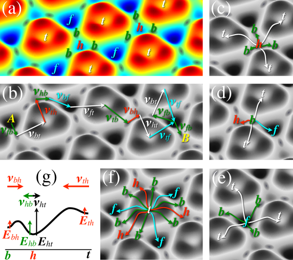
Figure 1: (a) Example of a complex potential energy landscape for a diffusing particle. Four adsorption site types are indicated: $f$, $h$, $t$ and $b$. (b) A possible diffusion track (random walk) involving 14 performed jumps with 10 different hop rates $\nu_{ij}$. (c)-(f) Possible hops from each site type ($h$, $b$, $f$ and $t$, respectively). Gray-shaded landscapes in (b)-(f) are used to highlight the colored arrows/hops. (g) Energy paths for hops starting/ending in $h$ sites. A longer arrow assigned to a hop rate ($\nu_{th}$, $\nu_{ht}$, etc…) indicates a larger rate.

We are interested in the low coverage regime, where the adparticle density is so low that the chance of affecting each other’s motion is negligible:

$$D^{\theta\approx 0}_{T}=\frac{1}{2\alpha}\lim_{t\rightarrow\infty}\frac{\left<|{\bf r}(t)-{\bf r}(0)|^{2}\right>}{t}.$$ (2)

The low coverage limit is an important measure as it provides a simple procedure to compare the typical distances covered by different adsorbates across different substrates [1, 2, 3, 4, 5]. Previous analytical work on diluted systems has focused on the determination of the center-of-mass diffusivity for small 2D islands and clusters on metal surfaces based on the master-equation [38, 39, 40] or the continuous time random walk formalism [41, 42]. In the framework of bulk-mediated surface diffusion, Revelli et al. described the average motion of the adsorbed molecules, including both Markovian and non-Markovian desorption, by using the generalized master-equation approach [43]. Birnie et al. [44] and Condit et al. [45] derived the overall jump rate for complex, sequential diffusion paths in three-dimensional (3D) crystals, where typical vacancy-interstitial complexes evolve by repeating a particular sequence of hops. The present study generalizes such sequential analysis by providing a universal expression for the diffusivity in complex hopping networks where both parallel and sequential diffusion routes are available between the different adsorption sites.

Computationally, adsorbate diffusion is traditionally studied by [1, 5]: (i) first principles calculations, typically involving the use of density functional theory (DFT) for the determination of the activation barriers and attempt frequencies, which are then passed to other methods; (ii) molecular dynamics simulations, which numerically solve Newton’s equations for the substrate and adsorbate atoms based on effective interaction potentials, enabling the analysis at the picosecond time scale for systems with $\sim$10⁵ atoms; (iii) Langevin models, which describe the adparticle in an effective periodic force field, restricting the analysis to general trends for time scales of picoseconds; and (iv) Kinetic Monte Carlo (KMC) simulations, which focus on describing the hops between adjacent basins (rare events) while disregarding all other vibrations, this way enabling long simulated times (seconds and minutes) with affordable computational resources. In this study we validate the proposed formulas for the diffusivity by direct comparison to KMC simulations in relevant energy landscapes, finally using the formulas to discuss the relative mobility and intercalation of various adsorbates in the context of topological insulators.

2 Theory

Let us consider a system with $S$ different site types, such as the one shown in figures 2(a) and 2(b) for $S=4$, or figure 2(c) for $S=3$. Although we assume diffusion in two dimensions, the underlying mathematical treatment and main result are also valid for three dimensions. For a generic hop from site type $i$ to site type $j$ ($i,j=1,...,S$) we consider that the hop distance $l_{ij}$, hop rate $\nu_{ij}$ and hop multiplicity $n_{ij}$ are known, and we define a new variable, the rateplicity $\mu_{ij}$, as the product of the rate and the multiplicity:

$$\mu_{ij}=n_{ij}\nu_{ij}\;.$$ (3)

We then propose that the low coverage diffusivity $D^{\theta\approx 0}_{T}$, as defined in equation 2, can be written as a weighted sum of partial diffusivities:

$$D^{\theta\approx 0}_{T}=\frac{1}{2\alpha}\Sigma_{i}w_{i}(\Sigma_{j}\mu_{ij}l_{ij}^{2})\;,$$ (4)

where $(\Sigma_{j}\mu_{ij}l_{ij}^{2})$ is the partial diffusivity from site $i$, which contains the rateplicities and hop lengths for all jumps from site type $i$ to any accessible site type $j$, and the dimensionless coefficient $w_{i}$ (or normalized weight for site $i$) stands for the probability to find the adatom at site type $i$:

$$w_{i}=\frac{B_{i}}{\Sigma_{j}B_{j}}\;\;\;(i=1,...,S),$$ (5)

where the $B_{i}$ coefficients consist of sums and products of rateplicities, their particular form depending on the number of adsorption sites $S$. As an example, for $S=2$ and $S=3$ we have:

$$\textstyle B_{i}= \textstyle\mu_{ji}\;\;\; \textstyle(S=2),$$ (6)

$$\textstyle B_{i}= \textstyle\mu_{ji}(\mu_{ki}+\mu_{kj})+\mu_{jk}\mu_{ki}\;\;\; \textstyle(S=3),$$ (7)

while a slightly more complex definition can be used for $S=4$:

$$\textstyle B_{i} \textstyle= \textstyle B_{ji}=B_{j^{\prime}i}\;\;\;(i\neq j\neq j^{\prime})$$ (8)

$$\textstyle B_{ij} \textstyle= \textstyle A_{ik}^{l}\mu_{kj}+A_{il}^{k}\mu_{lj}+U_{l}^{k}\mu_{ij}\;\;\;(i\neq j\neq k\neq l)$$ (9)

$$\textstyle A_{ij}^{k} \textstyle= \textstyle\mu_{ij}(R_{k}-\mu_{kk})+\mu_{ik}\mu_{kj}\;\;\;(i\neq j\neq k)$$ (10)

$$\textstyle U_{j}^{i} \textstyle= \textstyle(R_{i}-\mu_{ii})(R_{j}-\mu_{jj})-\mu_{ij}\mu_{ji}\;\;\;(i\neq j)$$ (11)

$$\textstyle= \textstyle A_{jk}^{i}+A_{jl}^{i}\;\;=\;\;\textstyle A_{ik}^{j}+A_{il}^{j}\;\;=\;\;\textstyle U_{i}^{j}$$ (12)

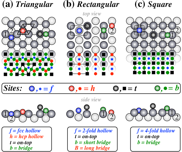
Figure 2: Schematic illustration of three typical surfaces with (a) triangular symmetry [e.g. fcc(111) and hcp(0001)], (b) rectangular symmetry [e.g. fcc(110)], and (c) square symmetry [e.g. fcc(100)]. We refer to typical adsorption sites as $f$ (for fcc hollow), $h$ (for hcp hollow), $t$ (for on-top), $b$ (for bridge/short bridge), and $B$ (for long bridge).

In practice, to determine each $B_{i}$ it is convenient to regard $i$ as the end site of a jump from a neighboring site $k$, so that $B_{i}=B_{ki}$, which is then determined by applying equations 9-11 ($S=4$) or equation 7 ($S=3$) or equation 6 ($S=2$). Any value of $k$ different from $i$ can be used since the $B_{ij}$ coefficients depend only on the second index ($B_{i}=B_{ki}=B_{k^{\prime}i}$, see equation 8). This is easily demonstrated by writing out $B_{ki}$ and $B_{k^{\prime}i}$ according to equation 9 and confirming their correspondence. For $S\geq 5$, a general procedure to determine the $B_{i}$ coefficients is described in the Supplementary Data, where also a rigorous derivation of equation 4 is provided. Valid for any value of $S$ in two and more dimensions, equation 4 is our central result.

Although equation 4 considers all $S\times S$ hops between all possible pairs from a set of $S$ different site types, non-occurring jumps can be eliminated from equation 4 by setting their rateplicities to zero ($\mu_{ij}=0$). This may lead, however, to undetermined values, e.g. $b_{i}=\frac{0}{0}$, and it is better to substitute the zeroed rateplicities by a small value ($\epsilon$) and take the limit $\epsilon\rightarrow 0$. As an example for the system shown in figure 1, if we consider only the $fh$, $ft$, $hf$, $ht$ and $tf$ hops (with multiplicity equal to 3) while disregarding all other hops, we may set $\mu_{ff}=\mu_{fb}=\mu_{hh}=\mu_{hb}=\mu_{th}=\mu_{tt}=\mu_{tb}=\mu_{bf}=\mu_{bh}=\mu_{bt}=\mu_{bb}=\epsilon$ in order to calculate the $B_{i}$ coefficients and then take the limit $\epsilon\rightarrow 0$ to determine the $b_{i}$ factors. We have:

$$\textstyle B_{f} \textstyle= \textstyle B_{hf}=B_{tf}=A_{th}^{b}\mu_{hf}+A_{tb}^{h}\mu_{bf}+U_{b}^{h}\mu_{tf}$$ (13)

$$\textstyle= \textstyle\epsilon(\mu_{hf}+\mu_{ht})\mu_{tf}+O(\epsilon^{2})$$ (14)

$$\textstyle B_{h} \textstyle= \textstyle B_{fh}=A_{ft}^{b}\mu_{th}+A_{fb}^{t}\mu_{bh}+U_{t}^{b}\mu_{fh}$$ (15)

$$\textstyle= \textstyle\epsilon\mu_{tf}\mu_{fh}+O(\epsilon^{2})$$ (16)

$$\textstyle B_{t} \textstyle= \textstyle B_{ht}=B_{ft}=A_{fh}^{b}\mu_{ht}+A_{fb}^{h}\mu_{bt}+U_{h}^{b}\mu_{ft}$$ (17)

$$\textstyle= \textstyle\epsilon(\mu_{fh}\mu_{ht}+\mu_{hf}\mu_{ft}+\mu_{ft}\mu_{ht})+O(\epsilon^{2})$$ (18)

$$\textstyle B_{b} \textstyle= \textstyle 0$$ (19)

Thus, using Equations 4 and 5 the diffusivity is:

$$\textstyle D^{\theta\approx 0}_{T} \textstyle= \textstyle\frac{1}{2\alpha}\frac{\left[B_{f}(\mu_{fh}+\mu_{ft})+B_{h}(\mu_{hf}+\mu_{ht})+B_{t}\mu_{tf}\right]l^{2}}{B_{f}+B_{h}+B_{t}}$$ (20)

$$\textstyle= \textstyle\frac{3}{2\alpha}\frac{2(\nu_{fh}+\nu_{ft})(\nu_{hf}+\nu_{ht})+\nu_{fh}\nu_{ht}}{\nu_{fh}(1+\frac{\nu_{ht}}{\nu_{tf}})+(\nu_{hf}+\nu_{ht})(1+\frac{\nu_{ft}}{\nu_{tf}})}l^{2}$$ (21)

Table 1: Examples of low coverage tracer diffusivities ($D^{\theta\approx 0}_{T}$) for different combinations of hop rates between standard adsorption sites on square, rectangular and triangular lattices. Site labels: f = 4-fold hollow (square) / 2-fold hollow (rectangular) / fcc hollow (triangular), h = hcp hollow (triangular), t = on-top, b = bridge (square) / short-bridge (rectangular) and B = long-bridge (rectangular). See the Supplementary Data for additional formulas.

Sym	Rate / multiplicity / distance	Geometry	$D^{\theta\approx 0}_{T}$ [$\alpha=2$]
Square	$\nu_{ff}$ $\nu_{ft}$ $\nu_{tf}$ $\nu_{tt}$ $4$ $4$ $4$ $4$ $l$ $d$ $d$ $l$		$\frac{4}{2\alpha}\frac{2\nu_{ft}\nu_{tf}d^{2}+(\nu_{tf}\nu_{ff}+\nu_{ft}\nu_{tt})l^{2}}{\nu_{ft}+\nu_{tf}}$
	$\nu_{ii}$ $\nu_{ib}$ $\nu_{bi}$ $\nu_{bb}^{d}$ $\nu_{bb}^{l}$ $4$ $4$ $2$ $4$ $2$ $2d$ $l/2$ $l/2$ $d$ $l$ $i=f$ or $i=t$	or	$\frac{4}{2\alpha}\frac{2\nu_{ib}\nu_{bi}\left(\frac{l}{2}\right)^{2}+2\nu_{ib}\nu_{bb}^{d}d^{2}+\nu_{ib}\nu_{bb}^{l}l^{2}+\nu_{bi}\nu_{ii}\left(2d\right)^{2}}{\nu_{bi}+2\nu_{ib}}$
	$\nu_{fb}$ $\nu_{tb}$ $\nu_{bf}$ $\nu_{bt}$ $4$ $4$ $2$ $2$ $l/2$ $l/2$ $l/2$ $l/2$		$\frac{4}{2\alpha}\frac{2\nu_{fb}\nu_{tb}(\nu_{bf}+\nu_{bt})}{2\nu_{fb}\nu_{tb}+\nu_{tb}\nu_{bf}+\nu_{fb}\nu_{bt}}\left(\frac{l}{2}\right)^{2}$
Rectangular	$\nu_{ff}^{l}$ $\nu_{ff}^{L}$ $\nu_{ft}$ $\nu_{tf}$ $\nu_{tt}^{l}$ $\nu_{tt}^{L}$ $2$ $2$ $4$ $4$ $2$ $2$ $l$ $L$ $d$ $d$ $l$ $L$		$\frac{2}{2\alpha}\frac{(\nu_{tf}\nu_{ff}^{l}+\nu_{ft}\nu_{tt}^{l})l^{2}+4\nu_{ft}\nu_{tf}d^{2}+(\nu_{tf}\nu_{ff}^{L}+\nu_{ft}\nu_{tt}^{l})L^{2}}{\nu_{ft}+\nu_{tf}}$
Triangular	$\nu_{ii}$ $\nu_{ij}$ $\nu_{ji}$ $\nu_{jj}$ $6$ $3$ $3$ $6$ $a$ $l$ $l$ $a$ $(i,j)=(f,h)$ or $(f,t)$ or $(h,t)$		$\frac{6}{2\alpha}\frac{\nu_{ij}\nu_{ji}l^{2}+(\nu_{ij}\nu_{jj}+\nu_{ji}\nu_{ii})a^{2}}{\nu_{ij}+\nu_{ji}}$
	$\nu_{fb}$ $\nu_{hb}$ $\nu_{tb}$ $\nu_{bf}$ $\nu_{bh}$ $\nu_{bt}$ $3$ $3$ $6$ $1$ $1$ $2$ $l/2$ $l/2$ $a/2$ $l/2$ $l/2$ $a/2$		$\frac{6}{2\alpha}\frac{\nu_{fb}\nu_{hb}\nu_{tb}(\nu_{bf}+\nu_{bh})\left(\frac{l}{2}\right)^{2}+2\nu_{fb}\nu_{hb}\nu_{tb}\nu_{bt}\left(\frac{a}{2}\right)^{2}}{\nu_{tb}(\nu_{hb}\nu_{bf}+\nu_{fb}\nu_{bh})+\nu_{fb}\nu_{hb}(\nu_{bt}+3\nu_{tb})}$
Sequential hops	$\nu_{12}$ $\nu_{23}$ $\nu_{31}$ $n$ $n$ $n$ $l$ $l$ $l$		$\frac{3n}{2\alpha}\frac{\nu_{12}\nu_{23}\nu_{31}}{\nu_{12}\nu_{23}+\nu_{23}\nu_{31}+\nu_{31}\nu_{13}}l^{2}$
	$\nu_{12}$ $\nu_{23}$ $\nu_{34}$ $\nu_{41}$ $n$ $n$ $n$ $n$ $d$ $d$ $d$ $d$		$\frac{4n}{2\alpha}\frac{\nu_{12}\nu_{23}\nu_{34}\nu_{41}}{\nu_{12}\nu_{23}\nu_{34}+\nu_{23}\nu_{34}\nu_{41}+\nu_{34}\nu_{41}\nu_{12}+\nu_{41}\nu_{12}\nu_{23}}d^{2}$

Table 1 shows a few example formulas obtained by applying equation 4 and the outlined $\epsilon\rightarrow 0$ procedure for various systems, including triangular, rectangular and square lattices. More detailed tables containing all relevant hop combinations for each lattice are provided as Supplementary Data. Although we restrict ourselves to the presentation of diffusivity expressions for 2D landscapes, equation 4 is completely general and can be applied to 3D problems as well. In fact, the last two equations of Table 1 for three and four sequential jumps, respectively, are identical to those derived by Condit et al. [45] and Birnie et al. [44], respectively, for vacancy diffusion in three dimensions. Our procedure, however, is more general, taking into account any number of competing diffusion paths from any given site (parallel processes) in addition to any number of successive hops along any given diffusion path (sequential processes).

3 Numerical validation

Based on the popularity of KMC simulations to determine tracer diffusivities [1, 2, 3, 4, 5, 36, 38, 46], we now compare the values obtained from the previous formulas and those determined by KMC simulations. As described in figure 3(a)-(b), we perform two types of simulations. In the first type (KMC-1) the tracer is followed until it hits the perimeter of a circle of radius $R_{o}\gg l_{ij}$, repeating the process for $N_{RW}$ different random walks (RWs) in order to obtain an ensemble average of the time $<t>$ required to cover that distance, thus determining the diffusivity as $D_{T}^{\theta\approx 0}=\frac{1}{2\alpha}\frac{R_{o}^{2}}{<t>}$. In the second type of simulations (KMC-2) the tracer is followed until it performs a desired number of hops $N_{H}$, repeating the process for $N_{RW}$ different RWs to determine the average squared distance $<X^{2}+Y^{2}>$ covered by the tracer and the corresponding average time $<t>$, obtaining the diffusivity by using $D_{T}^{\theta\approx 0}=\frac{1}{2\alpha}\frac{<X^{2}+Y^{2}>}{<t>}$.

Since the goal is to check the validity of the analytical expressions for the diffusivity, different hop rate values are used to probe situations where the rates have similar values / differ by several orders of magnitude. We also use realistic hop rates for several adsorbates, including Cu, Ag, Rb and Se on the Bi₂Se₃(0001) surface and in the vdW gap of this material. In this case the hop rates are expressed as $\nu=\nu_{0}e^{-E_{a}/k_{B}T}$, where the Boltzmann factor $e^{-E_{a}/k_{B}T}$ reflects the probability to perform the jump at temperature $T$ if the energy barrier is $E_{a}$, and $\nu_{0}$ is the attempt frequency, which reflects the dynamical coupling between the substrate phonons and the adparticle vibrations [1]. The actual values for these hop rates are obtained by determining the energy barriers through labor-intensive DFT calculations (see the Supplementary Data) and estimating the attempt frequencies by the method described in figure 3(c)-(e), leading to:

$$\nu_{o}\approx\nu_{L}^{A}\approx\frac{1}{2d}\sqrt{\frac{E_{a}}{2m}}.$$ (22)

Here, $E_{a}$ is the energy barrier for the hop, $d$ is the separation between the initial site $A$ and the saddle point $T$ (transition state) and $m$ is the adatom mass.

This estimate can be considered as an alternative to (i) the typical assumption of equal prefactors for all hop rates [1, 47, 48, 49, 46], and (ii) the large computational cost to determine all the vibrational mode frequencies $\nu_{i}^{A}$ and $\nu_{i}^{T}$ for the adatom and substrate at the initial and saddle configurations by using DFT methods [1, 47, 48, 49] (see expression ’U’ for the attempt frequency in figure 3(d)). Due to typical cancellations of the vibrational modes of the substrate [49], the prefactor $\nu_{o}$ is usually approximated by the Vineyard equation (expression ’V’ in figure 3(d)). Owing to compensation effects between the surface-parallel ($\nu_{\parallel}^{A}$ and $\nu_{\parallel}^{T}$) and surface-normal ($\nu_{\perp}^{A}$ and $\nu_{\perp}^{T}$) vibrational frequencies of the diffusing atom [49], the Vineyard formula is approximated by just keeping the frequency of the longitudinal vibrations (along the diffusion path) of the atom at the initial site ($\nu_{L}^{A}$, see expression ’W’ in figure 3(d)). Our estimate consists on approximating the longitudinal path by a sinusoidal path, resulting in a simple and physically meaningful expression for $\nu_{L}^{A}$ in terms of the energy barrier, hop distance and adatom mass, as described in figure 3(f) and contained in equation 22. Although the actual energy path can be asymmetric with respect to the saddle point T, the part after this point is irrelevant for the rate calculation and in our approximation it is considered to be a reflection of the part before it.

For all considered systems the simulated and calculated diffusivities agree extremely well with each other (see Table S5 of the Supplementary Data), thus concluding that the proposed formulas are suitable to discuss the low coverage tracer diffusivity of typical diffusion species in complex energy landscapes without any need to perform the corresponding KMC simulations.

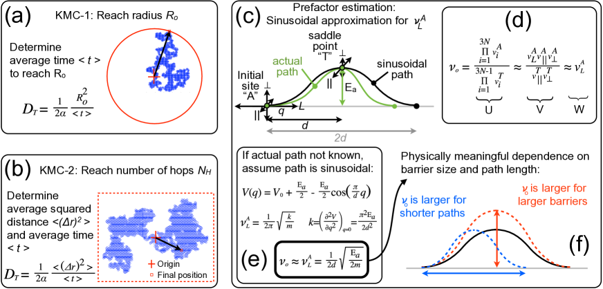
Figure 3: Illustration of the two simulation procedures used to perform KMC simulations of diffusion in this study: (a) KMC-1, (b) KMC-2. (c)-(e) Estimation of the attempt frequencies in this study. (f) Interpretation of the attempt-frequency dependence on the barrier size and path length.

4 Application to topological insulators

Encouraged by the validation of the diffusivity formulas we now consider the temperature dependence of the diffusion of Cu, Ag and Rb adatoms on the Bi₂Se₃(0001) surface and the corresponding intercalation of these adsorbates in the Bi₂Se₃ vdW gap. Figure 4(a)-(b) provides the calculated diffusion length $\Lambda=\sqrt{2\alpha D^{\theta\approx 0}_{T}t}$ as a function of temperature for the three considered adatoms when they diffuse on the surface and in the vdW gap, respectively. The evaluations have been done on the basis of the formulas obtained for $D^{\theta\approx 0}_{T}$ (see fifth column of Table S5 of the Supplementary Data). For diffusion with a single barrier $E_{a}$, the underlying assumption that the hops can be treated as rare events (as compared to the fast vibrations around the adsorption sites) is valid if $E_{a}>4k_{B}T$ (see Ref. [1]). Correspondingly, each displayed curve in figure 4 terminates at $T_{\rm max}=E_{a,{\rm max}}/4k_{B}$, where $E_{a,\rm max}$ is the maximum barrier experienced by the corresponding adatom. As an example, the diffusion of Rb on the surface experiences two barriers: $E_{fh}$ = 0.127 eV and $E_{hf}$ = 0.104 eV. Thus, $E_{a,{\rm max}}$ = 0.127 eV and $T_{\rm max}$ = 368 K. Similarly, for Cu in the vdW gap we have $T_{\rm max}$ = 342 K. Nevertheless, the total temperature range is restricted to 600 K since the desorption of Cu is reported to start at $\sim$550 K [50].

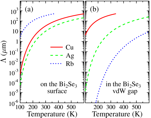
Figure 4: Calculated diffusion length $\Lambda$ (in logarithmic scale) as a function of temperature for Cu, Ag and Rb adatoms: (a) on the Bi₂Se₃(0001) surface, and (b) in the Bi₂Se₃ vdW gap. Diffusion time: 1 min.

It can be seen from figure 4 that the hierarchy of the diffusion length is $\Lambda_{\rm Rb}>\Lambda_{\rm Cu}>\Lambda_{\rm Ag}$ on the surface and $\Lambda_{\rm Cu}>\Lambda_{\rm Ag}>\Lambda_{\rm Rb}$ in the vdW gap. The Rb (Cu) atoms are the most mobile species on the surface (in the vdW gap), capable of covering more than 1 $\mu$m within one minute even at 100 K. However, the vdW (surface) diffusion length of the Rb (Cu) atoms is much lower than that on the surface (in the vdW), which is due to significantly higher diffusion barriers. Interestingly, the Ag atoms travel with almost equal rates on the surface and in the vdW gap.

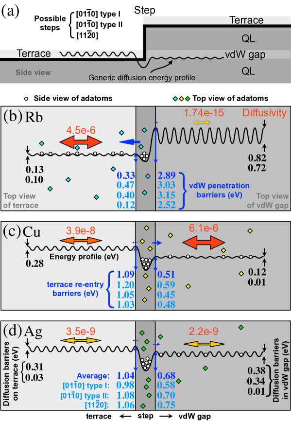
Figure 5: (a) Geometrical alignment between terrace and vdW gap at a morphological step. (b)-(d) Schematic representation of the low coverage diffusivity (in cm²s^-1) of Rb, Cu and Ag on the terrace and in the vdW gap of Bi₂Se₃ at room temperature. Larger arrows denote larger diffusivities. Our DFT-calculated diffusion barriers (in eV) are shown in boldface for: (left) terrace diffusion, (center-left) terrace re-entry, (center-right) vdW-gap penetration and (right) vdW-gap diffusion.

Let us now bring the discussion closer to the available experiments [21, 23, 30]. These indicate indirectly the occurrence of partial [21] or almost complete [23, 30] intercalation of the metal adatoms inside the Bi₂Se₃ vdW gap at room and higher temperatures. Recently, it has been argued [28] that the intercalation of the metal atoms in the Bi₂Se₃ vdW gap is step-mediated, in the sense that they penetrate into the vdW gap after reaching the steps, which are typically present at the Bi₂Se₃ surface [23]. This is favored by the geometrical alignment between the terrace and the vdW gap in a stepped surface, as schematically shown in 5(a). At the same time, penetration of Cu [23] and Ag [28] in the vdW gap via interstitials and/or vacancies of the topmost Bi₂Se₃ QL is significantly less probable due to high energy barriers. Therefore, one may also rule out the possibility of vertical penetration of the Rb atom, whose covalent radius is 1.5 (1.66) times larger than that of Ag (Cu), whereupon the diffusion barriers are expected to be even higher.

By using large and small double-head arrows, figure 5(b)-(d) presents a graphical description of the relative diffusivity of the three types of adatoms on the terraces and within the vdW gaps. In addition, the figure also provides the relative rates to enter the vdW gap and to bounce back to the terrace by assigning them large/small unidirectional arrows. Moreover, the figure collects all the diffusion barriers determined by our DFT calculations for the three adatoms on the terrace and in the vdW gap, as well as for their penetration into the vdW gap and re-entry into the terrace for two different step orientations, namely, [$11\bar{2}0$] and [$01\bar{1}0$], the latter having two possible atomic terminations [28]. To ease the discussion, the three barriers for vdW penetration (terrace re-entry) for each adatom are algebraically averaged and used to estimate the vdW penetration (terrace re-entry) rate of that atom, accordingly assigning them large/small unidirectional arrows. We center the discussion at room temperature (295 K) and long diffusion times.

The Rb atoms have the largest terrace and smallest vdW diffusivities, with a very low vdW-penetration rate and a rather large terrace-reentry rate. Thus, the Rb atoms are expected to quickly diffuse across the terraces and hit the steps, where a small fraction will remain trapped while the majority will bounce back to the terraces. This is described schematically in figure 5(b) by drawing a large number of Rb atoms in the terrace region, with additional atoms at the step, while hardly any atoms in the vdW gap. In comparison, the Cu atoms are characterized by moderate terrace and largest vdW diffusivities, with the largest vdW-penetration rate and a low terrace-reentry rate. Accordingly, the Cu atoms need a longer time to arrive at the steps but they eventually penetrate with relative ease into the vdW gap, where they diffuse rather fast. Thus, the Cu atoms are expected to mostly intercalate in the vdW gap, although a notable fraction will remain at the steps, as sketched in figure 5(c). Finally, the Ag atoms display slightly lower terrace diffusivity as compared to Cu and a medium diffusivity in the vdW gap among the three species under consideration. Having reached the steps, the Ag atoms are forced to linger along them due to the large terrace-reentry barrier and significant vdW-penetration barrier (figure 5(d)). Since the latter is smaller, the Ag atoms are expected to gradually intercalate into the vdW gap. The behavior is similar to that of Cu, although intercalation is slower for Ag. Valid only for the low coverage limit, these trends are in good qualitative agreement with those from available experiments [21, 23, 30].

5 Conclusion

Focusing on the analysis of adsorbate diffusion on surfaces and within the two-dimensional gap of layered materials, we present a combination of formulas for future reference and their application to intercalation in a topological insulator (Bi₂Se₃). We start by presenting a general expression to determine the average motion of the diffusing particles at low densities in complex, periodic energy landscapes consisting of various energy barriers located between distinct adsorption sites in any number of dimensions. For adsorbate diffusion in two dimensions, formulas are provided for the low coverage tracer diffusivity for complex combinations of hop rates in systems with triangular, rectangular and square symmetry. The analytical expressions are validated against Kinetic Monte Carlo simulations, obtaining an excellent agreement between the calculated and simulated diffusivities. Thus, one can determine the overall diffusion coefficient without performing the KMC simulations. Based on diffusion rates from energy barriers obtained by labor-intensive density functional theory calculations, we analyze the temperature dependence of the diffusion of Cu, Ag and Rb on the Bi₂Se₃(0001) surface and within the van der Waals (vdW) gap inside the (layered) crystal. We also analyze the occurrence of adsorbate intercalation due to the alignment between the vdW gaps and terraces on [11$\overline{2}$0]- and two types of [01$\overline{1}$0]-stepped surfaces of this topological insulator. At room temperature and low coverage, we conclude that the Rb atoms quickly diffuse across the terraces and hit the steps, where a small number remain trapped while the rest bounce back into the terraces. Thus, Rb is expected to partially decorate the steps while remaining present on the terraces. In comparison, the Cu atoms take a longer time to arrive to the steps, eventually penetrating with relative ease into the vdW gap. Thus, Cu atoms are expected to mostly intercalate into the vdW gap while partially remaining at the steps. Ag atoms are expected to take an even longer time to diffuse across the terraces, eventually penetrating into the vdW gap with time but meanwhile remaining around the steps.

References

References

- [1] Ala-Nissila T, Ferrando R, Ying S 2002 Collective and single particle diffusion on surfaces. Advances In Physics 51 949–1078.
- [2] Naumovets A, Zhang Z 2002 Fidgety particles on surfaces: how do they jump, walk, group, and settle in virgin areas? Surface Science 500 414–436.
- [3] Gomer R 1990 Diffusion of adsorbates on metal-surfaces. Reports On Progress In Physics 53 917–1002.
- [4] Kellogg G L 2001 Surface Diffusion at Solid Surfaces: An Atomic View (Elsevier), pp 9025–9030.
- [5] Ferrando R 2006 Surface Diffusion: Simulations (Elsevier), pp 1–6.
- [6] Ma Z, Zaera F 2006 Heterogeneous Catalysis by Metals (John Wiley & Sons, Ltd).
- [7] Li X, et al. 2009 Large-Area Synthesis of High-Quality and Uniform Graphene Films on Copper Foils. Science 324 1312–1314.
- [8] Bae S, et al. 2010 Roll-to-roll production of 30-inch graphene films for transparent electrodes. Nature Nanotechnology 5 574–578.
- [9] Bonaccorso F, et al. 2012 Production and processing of graphene and 2d crystals. Materials Today 15 564 – 589.
- [10] Xu M, et al. 2013 Graphene-like two-dimensional materials. Chemical Reviews 113 3766–3798.
- [11] Wang H, et al. 2012 Large-scale 2D electronics based on single-layer MoS2 grown by chemical vapor deposition IEEE International Electron Device Meeting (IEDM) 2012 Tech. Digest pp 4.6.1–4.6.4.
- [12] Lee Y H, et al. 2012 Synthesis of large-area MoS2 atomic layers with chemical vapor deposition. Advanced Materials 24 2320–2325.
- [13] Ismach A, et al. 2012 Toward the Controlled Synthesis of Hexagonal Boron Nitride Films. ACS Nano 6 6378–6385.
- [14] Ci L, et al. 2010 Atomic layers of hybridized boron nitride and graphene domains. Nature Materials 9 430–435.
- [15] Boscher N D, Carmalt C J, Parkin I P 2010 Atmospheric pressure chemical vapour deposition of NbSe2-TiSe2 composite thin films. Applied Surface Science 256 3178 – 3182.
- [16] Yan Y, et al. 2013 Synthesis and quantum transport properties of Bi2Se3 topological insulator nanostructures. Sci. Rep. 3 1264.
- [17] Li H, et al. 2012 Controlled synthesis of topological insulator nanoplate arrays on mica. Journal of the American Chemical Society 134 6132–6135.
- [18] Adroguer P, et al. 2012 Diffusion at the surface of topological insulators. New J. Phys. 14 103027
- [19] Bianchi M, et al. 2011 Simultaneous quantization of bulk conduction and valence states through adsorption of nonmagnetic impurities on Bi2Se3. Phys. Rev. Lett. 107 086802.
- [20] Zhu Z H, et al. 2011 Rashba Spin-Splitting Control at the Surface of the Topological Insulator Bi2Se3. Phys. Rev. Lett. 107 186405.
- [21] Bianchi M, et al. 2012 Robust Surface Doping of Bi2Se3 by Rubidium Intercalation. ACS Nano 6 7009–7015.
- [22] Valla T, et al. 2012 Photoemission spectroscopy of magnetic and nonmagnetic impurities on the surface of the Bi2Se3 topological insulator. Phys. Rev. Lett. 108 117601.
- [23] Wang Y L, et al. 2011 Structural defects and electronic properties of the cu-doped topological insulator Bi2Se3. Phys. Rev. B 84 075335.
- [24] Ye M, et al. 2012 Quasiparticle interference on the surface of Bi2Se3 induced by cobalt adatom in the absence of ferromagnetic ordering. Phys. Rev. B 85 205317.
- [25] Scholz M R, et al. 2012 Tolerance of topological surface states towards magnetic moments: Fe on Bi2Se3. Phys. Rev. Lett. 108 256810.
- [26] Seibel C, et al. 2012 Single Dirac cone on the Cs-covered topological insulator surface Sb2Te3(0001). Phys. Rev. B 86 161105.
- [27] Eremeev S V, Vergniory M G, Menshchikova T V, Shaposhnikov A A, Chulkov E V 2012 The effect of van der Waal’s gap expansions on the surface electronic structure of layered topological insulators. New J. Phys. 14 113030.
- [28] Otrokov M M, et al. 2013 Efficient step-mediated intercalation of Silver atoms deposited on the Bi2Se3 surface. JETP Letters 96 714–718.
- [29] Eelbo T, et al. 2013 Co atoms on Bi2Se3 revealing a coverage dependent spin reorientation transition. New J. Phys. 15 113026
- [30] Ye M, et al. 2011 Relocation of the topological surface state of Bi2Se3 beneath the surface by Ag intercalation http://arxiv.org/abs/1112.5869v1.
- [31] Koski K J, et al. 2012 Chemical intercalation of zerovalent metals into 2d layered Bi2Se3 nanoribbons. Journal of the American Chemical Society 134 13773–13779.
- [32] Hor Y, et al. 2011 Superconductivity and non-metallicity induced by doping the topological insulators Bi2Se3 and Bi2Te3. Journal of Physics and Chemistry of Solids 72 572 – 576.
- [33] Hor Y S, et al. 2010 Superconductivity in CuxBi2Se3 and its implications for pairing in the undoped topological insulator. Phys. Rev. Lett. 104 057001.
- [34] Wray L A, et al. 2010 Observation of topological order in a superconducting doped topological insulator. Nat Phys 6 855–859.
- [35] Diamantini M C, Sodano P and Trugenberger C A 2012 From topological insulators to superconductors and confinement. New J. Phys. 14 063013
- [36] Vattulainen I, Ying SC, Ala-Nissila T, Merikoski J 1999 Memory effects and coverage dependence of surface diffusion in a model adsorption system. Phys. Rev. B 59 7697–7707.
- [37] Vattulainen I, Merikoski J, Ala-Nissila T, Ying S C 1998 Adatom dynamics and diffusion in a model of O/W(110). Phys. Rev. B 57 1896–1907.
- [38] Salo P, et al. 2001 Role of concerted atomic movements on the diffusion of small islands on fcc(100) metal surfaces. Phys. Rev. B 64 161405.
- [39] Sanchez J R, Evans J W 1999 Diffusion of small clusters on metal (100) surfaces: Exact master-equation analysis for lattice-gas models. Phys. Rev. B 59 3224–3233.
- [40] Titulaer U, Deutch J 1982 Some aspects of cluster diffusion on surfaces. Journal of Chemical Physics 77 472–478.
- [41] Kley A, Ruggerone P, Scheffler M 1997 Novel diffusion mechanism on the GaAs(001) surface: The role of adatom-dimer interaction. Phys. Rev. Lett. 79 5278–5281.
- [42] Haus J, Kehr K 1987 Diffusion in regular and disordered lattices. Physics Reports 150 263–406.
- [43] Revelli J A, Budde C E, Prato D and Wio H S 2005 Bulk-mediated surface diffusion: non-Markovian desorption dynamics New J. Phys. 7 16
- [44] Birnie D 1990 Migration frequencies for complex diffusion paths. Journal of Physics and Chemistry of Solids 51 1313–1321.
- [45] Condit R, Hobbins R, Birchenall C 1974 Self-diffusion of Iron and Sulfur in Ferrous Sulfide. Oxidation of Metals 8 409–455.
- [46] LePage J G, Alouani M, Dorsey D L, Wilkins J W, Blöchl P E 1998 Ab initio calculation of binding and diffusion of a Ga adatom on the surface. Phys. Rev. B 58 1499–1505.
- [47] Ratsch C, Scheffler M 1998 Density-functional theory calculations of hopping rates of surface diffusion. Phys. Rev. B 58 13163–13166.
- [48] Yildirim H, Kara A, Durukanoglu S, Rahman T 2006 Calculated pre-exponential factors and energetics for adatom hopping on terraces and steps of Cu(100) and Cu(110). Surface Science 600 484–492.
- [49] Yildirim H, Kara A, Rahman T S 2007 Origin of quasi-constant pre-exponential factors for adatom diffusion on Cu and Ag surfaces. Phys. Rev. B 76 165421.
- [50] Ikeda T, Watanabe T, Itoh H, Ichinokawa T 1996 Surface structures and growth modes for Cu on Si(100), (110) and (111) surfaces depending on cu segregation by heat treatment. Surface Review and Letters 03 1377–1385.