The prospect of using LES and DES in engineering design, and the research required to get there

Abstract

In this paper we try to look into the future to envision how large eddy and detached eddy simulations (LES and DES, respectively) will be used in the engineering design process about 20-30 years from now. Some key challenges specific to the engineering design process are identified, and some of the critical outstanding problems and promising research directions are discussed.

1 Introduction

This paper is about the feasibility of using large eddy simulations (LES) and (to a somewhat lesser extent) detached eddy simulations (DES) in the industrial engineering design process about 20-30 years from now. Many practitioners of computational fluid dynamics (CFD) for realistic turbulent flows believe that the cost of LES is and will remain so high that it won’t truly enter the practical engineering design optimization process for another 30 years. Additionally, although anybody can create a grid and run an LES these days, detailed expertise is required to ensure that the result are trustworthy and to interpret the results. The verification process is either lacking or completely expert-driven, and requires large amounts of both human and computer time.

Prior to writing this paper, we communicated with CFD experts at different corporations in a range of business areas; one message was that, despite the difficulties, there is a true need for LES in design optimization. LES combines the advantages of simulations with (some of) the reliability of physical experiments. It gives engineers higher confidence in the results, especially in the complex flows typically occuring in optimized engineering devices (e.g., jet engine combustors) or near the edges of the operational envelope (e.g., an airfoil near stall), than the lower fidelity simulations primarily used today (i.e., RANS and URANS). With more accurate predictions for complex and off-design flows, engineers could push designs closer to the edge of the envelope with lower safety factors and possibly more optimal designs (faster, cheaper, greener, etc).

In this paper we try to look into the future to envision how LES will be used in the engineering design process about 20-30 years from now. The context of the industrial design process and the challenges this creates is discussed in section 2; the research required to get there is discussed in section 3. While our focus is primarily on LES, much of the discussion applies to DES as well.

At the outset, we want to be emphasize that this paper is not a review paper. We do not intend to cover all the available literature. As requested by the organizer of this special issue, we instead attempt to be “prophetic” – looking into the future to explore what we see as the key challenges of using LES in engineering design, and the research required to get to where we think LES should be in 20-30 years.

2 The challenges of using LES in engineering design

LES is a well-established and very commonly used tool within the academic community. It is certainly used by engineers in industry, but rarely within the actual design process; more often, LES is used in one-off situations or in industrial R&D studies.

It is crucial to appreciate just how different a design process is from an academic study. The goal of the latter is often to generate physical insight, and thus the fidelity and accuracy of the LES are very important. The typical academic study runs for 3-5 years, during which perhaps a handful of high-quality LES are performed.

The engineering design process is very different. The objective is to make the correct design decision, and later to certify this. The quality of any given simulation performed to support this design decision is of less importance, provided that it leads to the correct decision. The overall time-scale of the design process, from concept to finished product, may not be that different from academic studies, but the time-scale of decision-making on sub-systems certainly is.

Taking a big-picture view of the design process, the simulation-needs are clearly different at different stages. Choosing between different concepts may require very fast, low-fidelity tools. As the design converges towards an optimized final product, higher-fidelity tools may be required for the final optimization. LES combines the advantages of simulations with some of the trustworthiness of experiments; it clearly has a place somewhere in the design/optimization process. The question is where and how to integrate it with other tools.

2.1 The need for fast turn-around

I have not failed. I’ve just found 10,000 ways that won’t work – Thomas A. Edison

Engineers work fast, because they often evaluate many designs before finding one that works. They need to quickly evaluate new designs, starting from a CAD model, to a CFD mesh, to a flow solution, to the post-processed result. The relative maturity of many engineering fields contributes to this fact: we already know how to design things that are close to optimal, and the last few percent of performance are the most difficult to attain. This implies that many design candidates need to be assessed, but also that a relatively high degree of accuracy may be needed (to distinguish between those last few percent). The latter is a saving grace for LES, as it implies that it can be useful for design well before it becomes an over-night tool like RANS – as long as the added-value of an LES study is sufficiently greater than a RANS study, a longer turn-around time can be acceptable. Turn-around times of a few days are probably acceptable for many applications.

The speed that matters is that of the full simulation process, from CAD to grid to solution to verification to distilled results. All of these steps are currently bottlenecks, and all must be substantially improved in order to enable fast turn-arounds. Automation may become as important as speed: the cost of computer-time is ever decreasing, while the cost of (highly educated) human-time is ever increasing.

2.2 The need for more than a single prediction

Engineers have labored the iterative process of design optimization since the invention of the wheel. To engineer the best product, we design, assess, then keep redesigning and reassessing. For LES and DES to benefit engineering design, these techniques must be able to not only assess a single design, but help us make decisions as we iteratively redesign and reassess.

Critical to making these decisions is how the flow field depends on the design. We want to know how quantities of interest, which collectively quantify how good the design is, depend on the design variables that parameterize all possible designs. Knowing this dependence enables an engineer to focus more on designs that produce favorable flows while avoiding designs that induce undesirable ones. To understand this dependence requires more than a single prediction by a single simulation. It requires integrating LES with the tools of sensitivity analysis.

Particularly useful for efficient design optimization is local sensitivity analysis, which computes the derivatives of the quantities of interest with respect to the design variables. The derivatives are essential in driving gradient-based optimization algorithms. They enable these algorithms to improve a design more quickly than gradient-free ones, especially when there are many design variables.

Sensitivity analysis is also useful in uncertainty quantification (UQ), a key component of engineering design. It helps engineers measure how uncertain factors affect the performance of their design. These factors include manufacturing variability, operating conditions, aging and degradation. If they cause unacceptable effects in performance, engineers need to know so that they can take measures to control the source of uncertainty, or to make their design more robust.

Despite being useful, sensitivity analysis is problematic for LES and DES. As an example, one of the authors once spent more than a year developing a local sensitivity analysis code for LES in complex geometries, only to find it diverging even in the simplest of cases. He later discovered the cause of the problem: LES is a chaotic dynamical system, and its sensitivity diverges due to the “butterfly effect” of chaos. As further explained in Section 3.5, the divergent sensitivity prohibits engineers from using this efficient tool in design optimization and in uncertainty quantification. Overcoming this divergence and enabling efficient sensitivity analysis is an important challenge in making LES and DES suitable for engineering design.

2.3 Multi-fidelity parametric design

Iterative design offers not only challenges, but also an opportunity for LES and DES to guide how reduced-order models are used. Scientists and engineers have developed models of many levels of fidelity for flow fields. They range from models derived from physical insight, often represented as algebraic or ordinary differential equations, to potential flow models that solves steady and linear partial differential equation, to RANS which solves a set of steady but nonlinear partial differential equations. LES (and, to a lesser extent, DES) tops almost all models both in complexity and in fidelity. LES performed for one particular design reveals much flow physics, which should guide engineers in choosing a reduced-order model, and even in tuning these models to make them more accurate for similar designs.

LES and DES provide new opportunities in optimization methods. They force us to think of optimization beyond its classic definition, of minimizing an objective function that can be evaluated exactly at fixed cost. In a multi-fidelity design, different models evaluate the objective function with different accuracy. High fidelity models, like LES and DES, have additional sampling errors unless they run for infinite time. Optimization becomes a resource management problem of how to allocate computation time between low and high fidelity models, such that they jointly minimize an objective function that can be evaluated at various levels of fidelity at various costs.

In this view, the development of a large aircraft, which takes many years, can be viewed as a single optimization process. In its early stage, a wide range of designs are explored using low fidelity estimates of the objective functions and constraints. As the optimization converges, it uses higher fidelity tools, upgrading from simulations to wind tunnel models and ultimately to test flying full scale aircrafts. LES combines the efficiency of simulation and trust-worthiness of physical experiments. It surely has its place in optimization. The question is where it fits best, how it would first be integrated into the process, and how it would make the design process faster and the product better.

Optimization is very expensive, so it would be completely unreasonable to think that we will do optimization solely with LES or even DES in 20 years – but the challenge is instead to think of ways to do optimization where we can utilize the strengths of LES. Doing so collaboratively with other models is both a research opportunity and a challenge.

2.4 The next generation computer hardware

High performance computing gets 1000 times faster every 10 to 15 years. This trend has lasted for several decades, and is predicted to continue for the next 20 years. Studies at the US Department of Energy have proposed extreme numbers of energy-efficient cores running in parallel to achieve “exascale” computing [1, 2, 3]. This trend will accelerate future LES calculations with thousand-fold faster floating point operations, but will also challenge it with a high cost of communication and data movement and extreme penalties on serial algorithms.

One impact on LES is that it will likely make spatially implicit differencing and filtering schemes [4] less attractive. These schemes, like Fourier transforms, introduce global connectivities, which will presumably be barriers to exascale parallelism.

Another impact is that we will likely need intricate computer science in future CFD codes. When the 17 Pflop/s, 1.6M core, BlueGene/Q Sequoia supercomputer was deployed in 2012-2013, a few LES-type codes were tested on it. The code written by one of the present authors was run on Sequoia without modifications, and utilized about 6% of the peak flop-rate [5]; compare this to the very similar code by Rossinelli et al. [6] (winner of the 2013 Gordon Bell prize) which reached 55% of peak on the same machine with a similar algorithm (5th order WENO). To achieve this performance, they had to re-write their code with a new data layout to maximize memory locality. If such code- and platform-specific modifications become broadly necessary on exascale machines, then this will have a large negative impact on the ability of small research groups to write efficient code for large-scale simulations.

3 The research required to get there

There are clearly gaps between the current state-of-the-art in LES and the requirements outlined in the previous section. The exponential increase in computer power will help close these gaps, but clearly will not, by itself, be sufficient. Research that advances our LES technology is certainly required.

The following sections describe some research areas that we deem particularly important, promising and exciting. The topics vary in maturity: some have been part of LES for a long time, but with important unsolved problems; others are more novel research areas that we feel are particularly interesting.

3.1 Complex geometries

Real engineering systems have complex geometries. Therefore, it seems clear that any LES developments that are not applicable to complex and general geometries or to unstructured grids will not have much impact. Likewise, developments that cannot be efficiently implemented on massively parallel computers will likely be of limited value.

These may seem trivial statements, but significant chunks of our current state-of-the-art in LES does not satisfy them. For example, the dynamic procedure by Germano et al. [7] requires both filtering and averaging in order to work: the standard academic approach is to perform these steps in homogeneous directions, which of course does not work in general geometries. The Lagrangian averaging approach [8] solves the latter problem but not the former. While filtering in non-homogeneous directions is theoretically well defined, in practice it can lead to a loss in accuracy. For example, a Germano procedure with wall-normal filtering in a coarsely resolved laminar boundary layer would return a non-zero eddy viscosity – this error is generally not seen in academic studies where filtering is performed in homogenous directions only.

A related example is the group of methods that uses Germano’s dynamic procedure in a global sense, to average over the full domain to find a single, global model coefficient. This appears to work for academic test cases where a single type of flow occupies most of the domain, but seems questionable in realistic, complex situations with many different types of flow within the domain.

3.2 Wall-modeling

The computational cost of LES is essentially independent of the Reynolds number $Re$ for free shear flows, it is only weakly dependent on $Re$ for the outer portion (say, the outermost 90%) of turbulent boundary layers, but it becomes strongly dependent on $Re$ for the innermost layer (the viscous sublayer, the buffer layer and the bottom of the logarithmic layer). In fact, traditional LES, where the innermost layer is resolved, permits a grid that is maybe 4 times coarser than DNS in each spatial direction when applied to high-$Re$ boundary layers, thus a cost-saving of two orders of magnitude; while significant, this is hardly a game-changer, and to truly enable LES of high-$Re$ boundary layer flows one must model the innermost layer: this is known as “wall-modeling”. In a classic paper, Spalart et al. [9] estimated that about $10^{11}$ grid points would be needed for wall-modeled LES of a complete, swept wing at full-scale flight conditions. While intimidating, this is at least five orders of magnitude less than would be required for traditional LES [9]. The DES approach is a few orders of magnitude cheaper, but by modeling the full boundary layer it is susceptible to similar errors as traditional RANS models in non-equilibrium flows, particularly (and very importantly) separating boundary layers [10]. By modeling only the innermost part of the boundary layer, which is also the part expected to display the closest to universal behavior, wall-modeled LES is, in principle, capable of more accurate predictions.

For quite some time, the main outstanding problems in wall-modeling for LES have been (in the perhaps biased views of the authors): 1) the “log-layer mismatch”, in which errors near the wall lead to errors in the predicted skin friction by about 10%; 2) the inherent assumption of turbulent flow in the wall-models, which renders them inaccurate in laminar regions and incapable of predicting transition to turbulence; and 3) the assumption of equilibrium flow in the wall-models, which renders their accuracy in non-equilibrium flows (most notably, during flow separation) questionable. All of these issues are clearly critical for airfoil flows, and recent research has made progress on particularly the first two issues. The log-layer mismatch can be removed by decoupling the thickness of the modeled near-wall layer from the LES grid, thus producing very accurate predictions of skin friction [11]. This naturally impacts the accuracy of the predicted frictional drag of an airfoil, but also (and arguably more importantly) the predicted separation location at high angles-of-attack, by ensuring that the incoming boundary layer has the right near-wall momentum.

In more recent work, Bodart & Larsson [12] introduced a sensor into the wall-model, which utilizes information from the resolved LES region to decide whether the boundary layer is laminar or turbulent, and only applies the wall-model if the latter. This was shown to enable the prediction of a transitional turbulent boundary layer using wall-modeled LES, where the transition location was in very close agreement with DNS without being prescribed in any way. To show how this can be applied to realistic aerospace problems, a wall-modeled LES prediction of the flow around the MD 30P/30N multi-component airfoil at a realistic full-scale Reynolds number and $19^{\circ}$ angle-of-attack is shown in Fig. 1 (taken from [12]). The transition locations were truly predicted by the wall-modeled LES method, without being prescribed in any way.

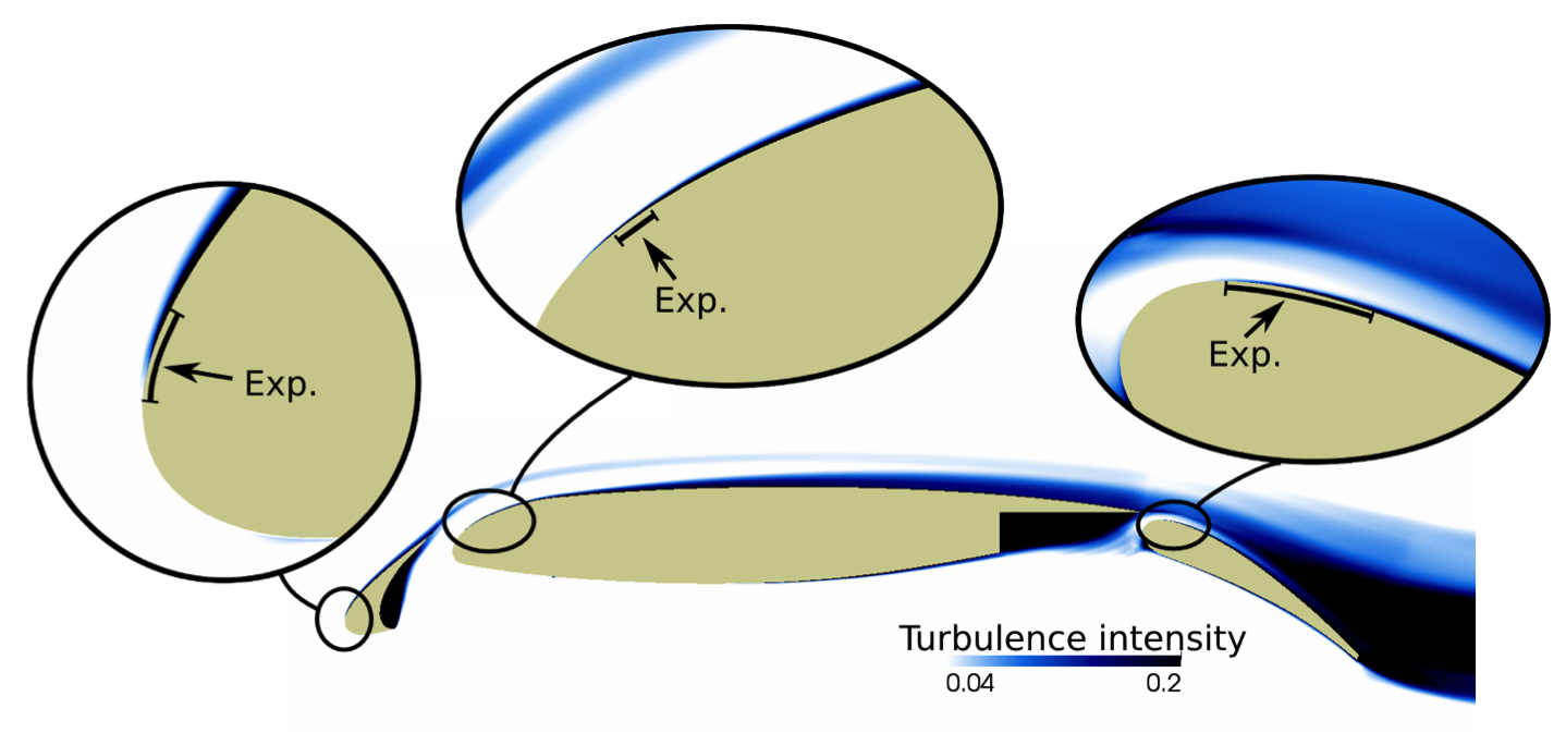
Figure 1: Predicting laminar-to-turbulent transition using wall-modeled LES on the MD 30P/30N airfoil with deployed slat and flap at $19^{\circ}$ angle-of-attack and chord Reynolds number of $Re_{c}=9\cdot 10^{6}$. The predicted transition occurs in the location, on each airfoil component, where the turbulence intensity rapidly increases to a finite value. The experimentally measured transition locations are indicated as ranges. Figure adopted from [12].

The question of how the assumption of equilibrium flow (basically: attached essentially parallel flow with small pressure gradient) in the wall-model affects the accuracy on strongly non-equilibrium problems (most importantly, separation) is less settled then one might imagine. While a separating boundary layer clearly is not in equilibrium, the wall-model is actually only applied within the innermost 10% or so of the boundary layer. Provided that most of the non-equilibrium effects are felt primarily in the outermost 90%, LES using an equilibrium wall-model might indeed be capable of very accurate predictions. Some very recent applications of wall-modeled LES to shock/boundary-layer interactions support this view [13], but much more research is needed to truly settle this matter. The focus should be on assessing the predictive ability of wall-modeled LES on separating and re-attaching boundary layers, and then, only if necessary, to develop more complex models.

3.3 Time integration

For the steady and unsteady RANS simulations used predominantly in industry today, fully implicit solvers are the most efficient. A fully implicit solver is more expensive (per time step) than a fully explicit method, but the latter is, of course, only stable for time steps smaller than some $\Delta t_{\rm stab}$. The exact cost difference between explicit and implicit methods depends strongly on the problem at hand, but for compressible viscous flows the difference can be many orders of magnitude. Simplistically, the fully explicit method is the more efficient one if the time step required for stability $\Delta t_{\rm stab}$ is no more than about 2-3 orders of magnitude smaller than the time step required for accuracy $\Delta t_{\rm accu}$.

Many academic test cases have simple geometries for which this is true (e.g., canonical free shear flows); for these problems a fully explicit method is a good choice. In other canonical problems this is violated by a linear term in a single direction (commonly, the wall-normal viscous diffusion in boundary layer flows); for such problems a linear line-implicit treatment is near-optimal in terms of computational efficiency. In many real-world problems, however, the time steps $\Delta t_{\rm stab}$ and $\Delta t_{\rm accu}$ differ by many, many orders of magnitude without there being any simple way to alleviate the problem; one thus faces a devil’s choice between taking millions of time steps using a fully explicit method, or living with the cost (operations and memory) of solving a fully implicit nonlinear system at every time step.

The wall-modeled LES of the MD 30P/30N discussed in section 3.2 and shown in Fig. 1 can serve as an example of this problem. Assume a chord of 10 m, which is typical of passenger jets. The laminar boundary layer near the nose of the slat is extremely thin due to the strong acceleration in that region, about 1 mm for our example; grid cells with a thickness of at most maybe 0.05 mm are required there to capture the transition process. The strong acceleration causes the flow to become near sonic above the slat, and thus a compressible solver is necessary; the stability limit for an explicit method is set by the wall-normal grid spacing divided by the speed-of-sound on the slat, about $\Delta t_{\rm stab}\approx$ 0.2 $\mu$s for our example (note that the viscous stability limit is much less severe for this example, by about a factor of $0.25\Delta y^{+}c/u_{\tau}$). To compute a single chord-passage might require 0.5M time steps, and many chord-passages are needed to wash out the initial transient.

To overcome this type of extreme numerical stiffness, a combination of numerical analysis and physical insight is needed. The nature of the stiffness is strongly related to physics and how different physics need to be resolved; thus a purely mathematical solution will likely not be optimal. Possible solutions include some form of selective implicit time stepping algorithm, where only some terms in some regions of the domain are treated implicitly. Done right, this should significantly decrease the cost of the implicit solver. Alternatively, the problem could be solved through local explicit time-stepping, with synchronization at regular intervals. One such algorithm for LES was presented recently by Lu et al. [14]. Whatever the approach, in addition to physics-induced stiffness (like for the MD 30P/30N airfoil), the time-stepping algorithm must also be able to handle stiffness due to poor grids: when meshing a complex geometry, it is difficult or impossible to avoid a handful of “bad cells” that might induce tremendous stiffness.

The potential speed-up of improved time-integration methods is bounded by how much more costly a fully implicit method is compared to an explicit one; for many LES problems, a speed-up of about two orders of magnitude should be possible.

3.4 Turbulent inflow and initial conditions

In many applications, one would like to perform LES in only a small subset of the total domain. Consider a turbofan jet engine: the flow through the inlet and the compressor is likely sufficiently well captured by RANS, but the turbulent reacting flow in the combustor would benefit from being treated by LES [15, 16]. There are many other examples.

To perform LES in only a limited part of the domain, one key difficulty is the boundary conditions, most notably the inflow condition. Being specified from a lower-fidelity method (RANS or other), the fluctuating flow will necessarily be approximate in nature. LES, however, is not accurate until the resolved turbulence is realistic, with realistic amplitudes, phase relationships and spectrum; this occurs after an adjustment region of length $L_{\rm adj}$, the value of which depends on the fidelity and realism of the inflow turbulence [17, 18, 19, 20]. With poor inflows, $L_{\rm adj}$ may be longer than the region one wants to study; this is clearly a bottleneck holding up the use of LES on sub-systems within larger, complex systems.

For canonical problems, the recycling/rescaling method of Lund et al. [21] and its many later improved versions has enjoyed significant success. By utilizing the resolved turbulence within the LES itself coupled with known scaling relationships, very realistic turbulence can be specified at the inlet. For complex engineering problems, however, we still need something better, since the rescaling relationships are then no longer valid.

The inflow problem is related to the problem of requiring long computation times just to get rid of the initial transients $T_{\rm init}$. A minimum required $T_{\rm init}$ is for the turbulence to pass through the domain once; this is proportional to the length of the domain, and thus a poor inflow may actually increase the cost in a quadratic manner (more grid points and longer $T_{\rm init}$). More generally, some flows require realistic initial conditions as well, with the required $T_{\rm init}$ strongly dependent on the fidelity of the initial turbulence (channel and pipe flows come to mind).

Finally, for compressible turbulence, the initial and inflow conditions will generate acoustic and entropy waves in addition to the hydrodynamic turbulence. Depending on the exact method, the level of acoustics may be one or two orders of magnitude larger than in “quiet” turbulence [22, 23]. In some applications (airframe noise, high-speed transition, …) this is a real problem.

Progress on any of these fronts would give us a greater ability to aggressively apply LES (or DES) only to the sub-systems or small portions of the domain where LES is truly needed. With current inflow technologies, whatever accuracy is gained by the sub-domain LES may be lost due to the errors incurred at the RANS $\rightarrow$ LES interface.

3.5 Grid-adaptation

In complex geometries, the grid generation process may become very time-consuming, particularly if high-quality grids that both minimize numerical errors (smooth grid transitions, low element skewness, etc) and provide sufficient resolution are needed – which they are, since we need trustworthy results for design decision-making. Adaptive grid-refinement, an iterative process in which the solution guides how the grid is adapted through some algorithm (rather than an expert user), is a somewhat mature technique within steady state simulations (including RANS); for LES, however, automatic, algorithm-driven grid-adaptation is a new area of research.

While grid-adaptation for RANS is solely aimed at reducing the numerical errors, it reduces both the numerical and subgrid modeling errors in LES as well as increases the fraction of resolved motions. This differentiates the problem from existing steady-state approaches, and poses new challenges. Pope [24] suggested adaptation targeted to resolving a user-defined fraction of the kinetic energy. The many existing unsteady adaptive mesh refinement (AMR) algorithms are most commonly used in moving-front problems (explosions, flames, shocks, …) for which the adaptation criteria are quite different from those of broadband turbulence.

To illustrate both the importance and difficulty of the grid-generation process in LES, consider Fig. 2 which shows some sample results from an attempt to perform LES of the reacting flow in a scramjet combustor. The “coarse” grid in the figure was the initial grid. Local grid-refinement (completely user-driven) to better resolve different flow features was then attempted; this was initially focused on the fuel injection and mixing region, but after much trial-and-error it became clear that the grid resolution in the region where the bow shock interacts with the side wall boundary layer (indicated by the circular shape in the figure) was actually equally important – without refinement there, the shocks reflected back along the centerline in the wrong place, thus causing delayed pressure rise (from $x\approx 100$ mm to $x\approx 120$ mm). It is difficult even for experienced users to anticipate exactly what grid resolution is required in different regions, and thus a more mathematical approach to this problem would quite clearly be very useful.

\begin{overpic}[width=469.47046pt,clip={true},trim=0.0pt 0.0pt 0.0pt 475.16101pt]{viz_cesco_mesh5_y8_schlieren_logscale.png} \put(36.0,22.0){\color[rgb]{0,0,1} \qbezier(4.0,0.0)(4.0,4.0)(0.0,4.0)\qbezier(0.0,4.0)(-4.0,4.0)(-4.0,0.0)\qbezier(-4.0,0.0)(-4.0,-4.0)(0.0,-4.0)\qbezier(0.0,-4.0)(4.0,-4.0)(4.0,0.0)} \end{overpic}

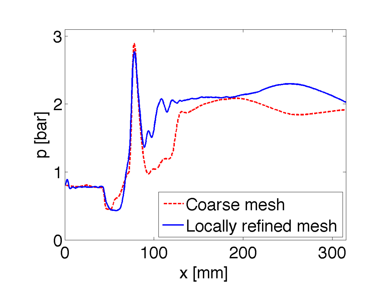
Figure 2: Illustrating the difficulty of generating grids that resolve the right features in the right places. The model scramjet combustor by Gamba et al. [25], with air at Mach 2.8 and 1100 K entering from the left and mixing with hydrogen injected from the bottom. The shocks and fuel/oxidizer mixing layers are seen in the simulated Schlieren images. The circular shape shows the main shock/boundary-layer interaction on the side wall, to be discussed in the text. To the right is shown the average pressure along the top wall from LES on two grids with 6M and 48M cells, respectively. The refinement was done in a manual, user-defined way, guided solely by experience and trial-and-error; the consequence of this is discussed in the text.

3.6 Sensitivity analysis of chaotic flow simulations

Sensitivity information, most obviously the gradient of the quantity-of-interest with respect to all design variables, is essential to optimization algorithms, uncertainty estimates and analyses of how robust a design or prediction is. The finite difference method to obtain sensitivites is popular and easy to implement, but is surprisingly problematic in LES and DES. This method approximates derivatives by selecting a pair of adjacent design points, then evaluating the quantity-of-interest at these points, and dividing their difference by the distance between the design points. Most quantities-of-interest are mean quantities, and computed (i.e., sampled) averages converge to the true mean at a rate of $T_{\rm avg}^{-1/2}$ due to the central limit theorem of statistics. When both objective functions are polluted by sampling errors due to finite time-averaging, the resulting derivative is polluted by a large error, specifically twice the sampling error divided by the distance between the design points. Reducing this error sufficiently for accurate sensitivity information could require impractically long simulations due to the very slow rate of convergence.

An example of this issue is shown in Fig. 3, which shows a specific quantity-of-interest $J$ and how this varies in time and with the design parameter $s$ for the Lorenz system (for this problem, $J$ is simply the value of the third variable while $s$ is the Rayleigh number). When computed as an initial value problem, nearby trajectories (starting from the same initial condition but having slightly different values of $s$) stay close for about 2-3 units of time and then rapidly become completely uncorrelated. When averaged, the uncorrelated sampling error results in a noisy $\overline{J}(s)$ function which could not be differentiated in any meaningful way.

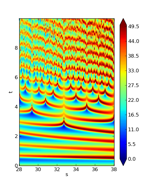
(a) Instantaneous $J(t,s)$, computed as an initial value problem.

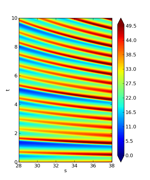
(b) Instantaneous $J(t,s)$, computed as a shadowing problem.

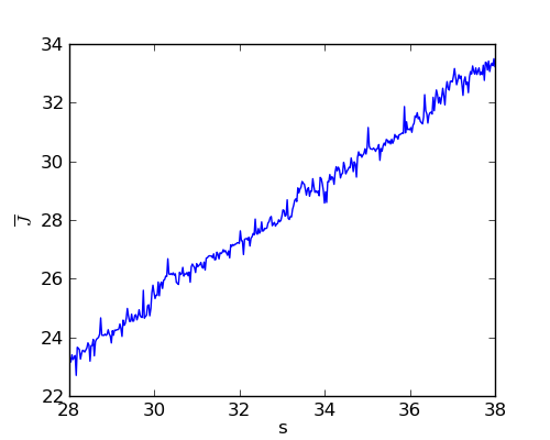
(c) Time-averaged $\overline{J}(s)$ of the initial value problem.

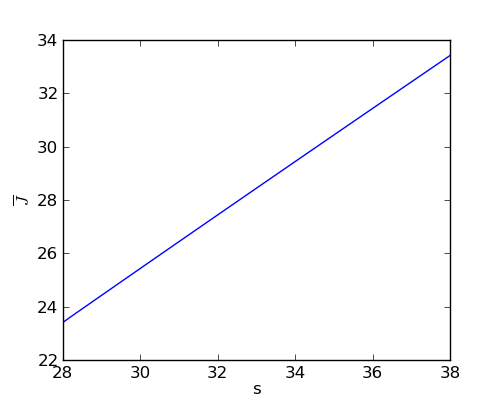
(d) Time-averaged $\overline{J}(s)$ of the shadowing problem.

Figure 3: Illustration of sampling errors when computing sensitivities in a chaotic system (the Lorenz system). The output functional $J$ as it varies with the design parameter $s$. The time-averages in the lower figures were computed over the full extent of time $t\in[0,10]$ in the upper figures. The “noise” in the left figures is the exponential divergence of nearby trajectories (slightly different values of $s$) – the “butterfly effect”.

In addition to the sampling error, the more standard problem with finite difference sensitivities is that they require $N+1$ simulations for $N$ design variables. To overcome this limitation, Jameson [26] introduced the adjoint method into CFD. By simultaneously computing the derivative to many design variables, the adjoint method has become widely used in aerodynamic design optimization. In LES and DES, however, the adjoint method encounters a fundamental challenge: the “butterfly effect” of chaotic dynamics.

By resolving the large scales of turbulence, LES inherits the chaotic dynamics characteristic of turbulence. A small perturbation, perhaps a slightly different mesh, can utterly change the time history of a simulation. This sensitivity to small purturbations (the “butterfly effect”) causes the adjoint method to diverge when integrated over a long time period $T$. The divergent adjoint solutions, observed in a variety of flow solvers [27, 28, 29], at first seem to suggest that perturbing the design always produces unbounded effects, even on long-time averaged statistics. This, of course, is not true: we know from experience that a quantity-of-interest (properly: a statistic) is, under the ergodic assumption, sensitive only to the design parameters and not to the exact realization (i.e., the initial condition). The differentiability of ergodic statistics to a design parameter can be proven under strict assumptions [3].

When computing the adjoint, however, the linearization inherent in the definition of the adjoint implies that it is defined following the specific solution trajectory along which it is computed. The positive Lyapunov exponent(s) of chaotic systems implies that there exists exponentially diverging trajectories; this causes the adjoint to diverge as well.

To overcome this problem, we must decouple the sensitivity of statistics from the realization of the flow field. A promising approach to this question is the shadowing approach [30]. The idea is to linearize the governing equation of an LES or DES, but not the initial condition. Liberated from the initial condition, the resulting linearized equation has many solutions. They describe how different the flow over a fixed pair of similar designs can be. Almost all these solutions diverge exponentially, but some of them do not. The ones that stay bounded are called shadowing solutions – they follow or “shadow” a given trajectory (see Fig. 4). As the length of the simulation increases, not only does a time averaged quantity converge to the infinite time average, but also its computed derivative converges to the derivative of the infinite time average [30].

Figure 4: Illustration of the shadowing paradigm, breaking causality: different trajectories in the Lorenz system at different values of the parameter $s$ (shown with different colors). Note that the output functional $J$ in Fig. 3 is simply the average vertical position in this plot, thus clearly showing a variation in $J$ for different $s$.

The Least Square Shadowing method and its adjoint has been applied to a range of dynamical systems, the largest being an isotropic homogeneous turbulent flow simulation at Taylor microscale Reynolds number $Re_{\lambda}=33$ by a $32^{3}$ Fourier pseudo-spectral discretization [31].

Without useful sensitivities of long-time averaged quantities, engineers are forced to drastically reduce the number of design variables, therefore significantly reducing the utility of LES. How to compute useful gradients in design-variable space, so that gradient-based optimization can be applied to LES and DES, is a key research question.

In addition to enabling gradient-based optimization, sensitivities would constitute an important component in a more rigorous uncertainty estimation and solution verification framework. This is also true for grid-adaptation methods.

3.7 Space-time parallelism

The growth of computing power is projected to continue primarily through increasing parallelism, as has been the case for more than a decade now. The CFD community has primarily harnessed this growth through use of spatial domain decomposition, but this strategy will become insufficient at some point. Most algorithms are efficiently parallelized only for sufficiently many cells per compute-process (core, thread, …) $n=N/p$, where $N$ and $p$ are the total number of cells and compute-processes, respectively. Thus there is a lower bound on the total wall-clock time that is proportional to the number of time steps $N_{t}$, which typically grows with $N$ for stability and accuracy reasons.

This may seem a distant problem, but it is arguably already becoming an issue for certain problems. For example, Pirozzoli and Bernardini (personal communication and [32]) used 11M cells and needed 2M time steps to capture the low-frequency oscillations in a shock/boundary-layer interaction problem. If the minimum useable $n$ is 1000, and a rather typical 50 $\mu$s per cell and time step is required by the solver, then this calculation cannot be completed in less than 28 hours on any machine available today – despite the modest grid size. And increasing the resolution would make it correspondingly worse, at a rate of about $\sim N^{1/3}$. Assuming continued growth in our appetite for ever larger grids, there is an upper bound to the benefits possible from extreme spatial parallelization. One possible answer is to improve the floating-point utilization of our codes (section 2.4); another is to parallelize the simulation in time as well as in space.

A space-time parallel simulation partitions the 4D space-time, with each resulting subdomain assigned to a computing process as illustrated in Fig. 5.

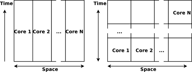
Figure 5: Illustration of spatial (left) and space-time (right) parallelism.

Time domain decomposition methods have a long history [33]. They include the multiple shooting method, the time-parallel and space-time multigrid methods, and the Parareal method. These methods start by computing an initial estimate of the solution (in space and time) using a cheap, reduced-order solver. This is then refined iteratively until it converges to the solution of the initial value problem. The key point is that this is done in parallel, i.e., different chunks of time are iterated upon simultaneously.

This approach becomes problematic, however, for chaotic initial value problems. The “butterfly effect” implies that the late-time solution is (instantaneously) very sensitive to the solution at early times. It would therefore be futile to even start iterating at the very late times before having reached a converged solution at early times; this, of course, destroys the parallel efficiency of the method. Although some turbulent initial value problems (plasma turbulence) have been successfully parallelized by the Parareal method [34, 35], there is clearly an upper bound.

To achieve efficient time domain parallelism for chaotic problems, we need to forsake the initial value problem and break causality. Unlike current simulations in which the past completely determines the future, a causality-breaking simulation allows for the future to determine the past – it modifies the past to resolve conflicts in the future. It computes the solution in a way not unlike how this paper was written: first a rough initial draft (cheap initial solver), then iterative refinements to all sections (solutions on finer grids) coupled with modifications to early sections to ensure consistency in the later sections (modifying the early solution to ensure that the governing equations are satisfied at later times).

Mathematically, the causality-breaking solution is defined as the solution closest (in the $L_{2}$-norm) to the initial guess that exactly satisfies the governing equation. The process is illustrated in Fig. 6. The initial guess is obtained by a reduced-order model and therefore does not satisfy the governing equation. Both the causality-enforcing and -breaking approaches reach final solutions that satisfy the governing equation, but do so very differently: in the former, the small changes required at early times propagate through the butterfly effect to produce very large changes at the late times. In contrast, only small changes are required in the causality-breaking case, and (crucially) these changes are essentially local-in-time.

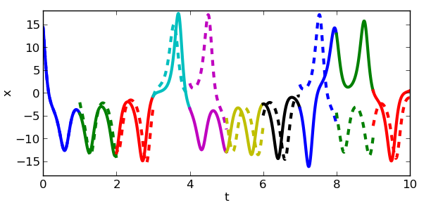
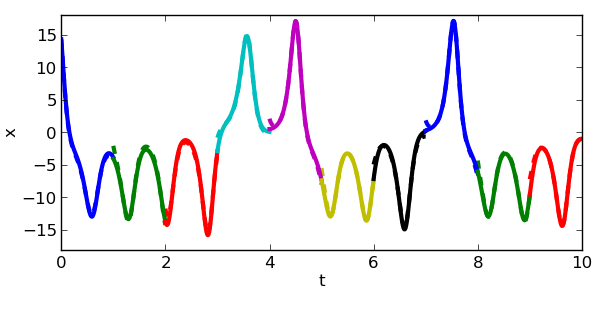
Figure 6: Two different solutions to the Lorenz system (solid lines) starting from the same initial guess (dashed lines). The left plot enforces causality while the right one breaks it. Each color represents a time chunk that can be handled by a different computing core. The initial guess is inconsistent at the time chunk boundaries, and the converged solution must resolve all these inconsistencies. Note that the causality-enforcing simulation must make global, large changes to resolve small inconsistencies, while the causality-breaking simulation only need to make small, local changes.

If this causality-breaking approach to time-parallelization could be made to work on real LES problems, then it would make LES truly scalable for ever larger problems and supercomputers. More importantly, it would enable the solution of moderate-size (i.e., engineering design) problems almost arbitrarily fast using extreme parallelization.

3.8 Putting new LES technologies into engineering practice

The preceeding sections listed some of the technical issues and research areas the authors feel are particularly important and/or promising in order to bring LES into practical use. In addition, we must become better at transitioning technologies from Academia to corporate research labs and eventually to engineering design.

The LES community has not been as successful at this as several other communities. For example, the SST, SA and V2F turbulence models are all about 20 years old, but have penetrated into most commercial CFD packages and many engineering design processes. The FFTW and Lapack libraries and the ParaView and VisIt visualization toolkits were also developed within the last 20 years or so; they have become important enabling technologies used in a wide range of fields. In that same time frame, the LES community developed subgrid models, wall-models, non-dissipative numerics, turbulent inflows and many other things – and yet the impact of LES on engineering design has been much smaller. So why have LES technologies been adopted more slowly, and what can be done to speed things up?

While academic researchers should never become applied engineers, we can and should make sure that the techniques we develop are applicable to real engineering problems. Novel modeling techniques should be fundamentally sound, and should be thoroughly tested on canonical problems where detailed assessment is possible, but we should keep the final application in mind. For example, if a subgrid model needs homogeneous directions for filtering and/or averaging, then its use in most realistic geometries becomes impossible.

The transitioning of knowledge should also include the transitioning of enabling technologies, particularly computer code. When the tax-paying public pays for a research project, it seems fair that any code generated as part of it becomes publically available; more to the point, this would enable further research at other institutions, which surely should be our goal. Progress on this front will come down to whether our funding agencies and program managers start demanding it.

Ultimately, the LES community, academic and industrial, would benefit from having a few well-documented, modular and capable open-source codes. OpenFOAM is a great example, but there is room for additional codes using different modularization paradigms and languages. Witness the impact of Matlab, which democratized matrix manipulations, and imagine how CFD and LES research across the world could be elevated by eliminating the constant drudgery of re-inventing the basic unstructured CFD code.

4 Final words

When considering the role of LES in engineering design in 30 years, one might wonder whether we will be able to replace RANS with LES throughout the design process? This is the wrong question to ask, and the answer is “no” anyway. Better questions are: “how and where in the process should we utilize LES to enable better decision-making?” and “for which sub-systems or sub-domains would LES substantially increase our trust in the predictions?”. Phrased this way, three “answers” or observations emerge quite clearly to the present authors: 1) there will definitely be a role for LES; 2) further advancement of the LES technology is needed to enable these kinds of studies (e.g., technology enabling LES in a sub-domain with accurate RANS $\leftrightarrow$ LES coupling); and 3) beyond technology advancements, we need to show success stories where LES clearly impacted design decision-making.

Several challenges multiply to make the use of LES in the engineering design process difficult. This is actually good news – it means that progress on these fronts, when combined, can have a large effect on the feasibility of using LES in design optimization. If improved time-stepping reduces the computational cost by a factor of 10, time-parallelization makes it possible to efficiently utilize 10 times more cores, and multi-fidelity optimization frameworks reduce the required number of LES runs by another factor of 10, then engineering LES will become 1000 times faster. A good grid-adaptation framework would drastically reduce the human-time required to build grids and simultaneously increase the quality of the computed results. Wall-models enable computations at realistic Reynolds numbers, and methods to compute sensitivities enable optimization and uncertainty estimation. And surely there are other areas in which improvements can be made. We are optimistic.

References

- [1] P. Kogge, K. Bergman, S. Borkar, D. Campbell, W. Carson, W. Dally, M. Denneau, P. Franzon, W. Harrod, K. Hill, et al., Exascale computing study: Technology challenges in achieving exascale systems (2008).
- [2] S. Amarasinghe, D. Campbell, W. Carlson, A. Chien, W. Dally, E. Elnohazy, M. Hall, R. Harrison, W. Harrod, K. Hill, et al., Exascale software study: Software challenges in extreme scale systems, DARPA IPTO, Air Force Research Labs, Tech. Rep.
- [3] D. Ruelle, Differentiation of SRB states, Comm. Math. Phys. 187 (1997) 227–241.
- [4] S. K. Lele, Compact finite difference schemes with spectral-like resolution, J. Comput. Phys. 103 (1) (1992) 16–42.
- [5] I. Bermejo-Moreno, J. Bodart, J. Larsson, B. M. Barney, J. W. Nichols, S. Jones, Solving the compressible Navier-Stokes equations on up to 1.97 million cores and 4.1 trillion grid points, Proc. SC13, 2013.
- [6] D. Rossinelli, B. Hejazialhosseini, P. Hadjidoukas, C. Bekas, A. Curioni, A. Bertsch, S. Futral, S. J. Schmidt, N. A. Adams, P. Koumoutsakos, 11 PFLOP/s simulations of cloud cavitation collapse, Proceedings of SC13, 2013.
- [7] M. Germano, U. Piomelli, P. Moin, W. H. Cabot, A dynamic subgrid-scale eddy viscosity model, Phys. Fluids 3 (7) (1991) 1760–1765.
- [8] C. Meneveau, T. S. Lund, W. H. Cabot, A Lagrangian dynamic subgrid-scale model of turbulence, J. Fluid Mech. 319 (1996) 353–385.
- [9] P. R. Spalart, W.-H. Jou, M. Strelets, S. R. Allmaras, Comments on the feasibility of LES for wings, and on a hybrid RANS/LES approach, in: C. Liu, Z. Liu (Eds.), Advances in DNS/LES, Greyden, Columbus, OH, 1997.
- [10] J. Slotnick, A. Khodadoust, J. Alonso, D. Darmofal, W. Gropp, E. Lurie, D. Mavriplis, CFD vision 2030 study: A path to revolutionary computational aerosciences.
- [11] S. Kawai, J. Larsson, Wall-modeling in large eddy simulation: length scales, grid resolution and accuracy, Phys. Fluids 24 (2012) 015105.
- [12] J. Bodart, J. Larsson, Sensor-based computation of transitional flows using wall-modeled large eddy simulation, in: Annu. Res. Briefs, Center for Turbulence Research, 2012, pp. 229–240.
- [13] I. Bermejo-Moreno, L. M. Campo, J. Larsson, J. Bodart, D. B. Helmer, J. K. Eaton, Confinement effects in shock wave/turbulent boundary layer interactions through wall-modeled large-eddy simulations, J. Fluid Mech. submitted.
- [14] Y. Lu, K. Liu, W. N. Dawes, Large eddy simulations using high order flux reconstruction method on hybrid unstructured meshes, AIAA Paper 2014-0424, 2014.
- [15] J. U. Schlüter, H. Pitsch, P. Moin, Large-eddy simulation inflow conditions for coupling with Reynolds-averaged flow solvers, AIAA J. 42 (2004) 478–484.
- [16] G. Medic, G. Kalitzin, D. You, M. Herrmann, F. Ham, E. van der Weide, H. Pitsch, J. Alonso, Integrated RANS/LES computations of turbulent flow through a turbofan jet engine, in: Annu. Res. Briefs, Center for Turbulence Research, 2006, pp. 275–285.
- [17] P. Batten, U. Goldberg, S. Chakravarthy, Interfacing statistical turbulence closures with large-eddy simulation, AIAA J. 42 (3) (2004) 485–492.
- [18] A. Keating, U. Piomelli, E. Balaras, A priori and a posteriori tests of inflow conditions for large-eddy simulation, Phys. Fluids 16 (12) (2004) 4696–4712.
- [19] S. Xu, M. P. Martin, Assessment of inflow boundary conditions for compressible turbulent boundary layers, Phys. Fluids 16 (7) (2004) 2623–2639.
- [20] L. di Mare, M. Klein, W. P. Jones, J. Janicka, Synthetic turbulence inflow conditions for large-eddy simulation, Phys. Fluids 18 (2006) 025107.
- [21] T. S. Lund, X. Wu, K. D. Squires, Generation of turbulent inflow data for spatially-developing boundary layer simulations, J. Comput. Phys. 140 (1998) 233–258.
- [22] J. R. Ristorcelli, G. A. Blaisdell, Consistent initial conditions for the DNS of compressible turbulence, Phys. Fluids 9 (1) (1997) 4–6.
- [23] J. Larsson, Blending technique for compressible inflow turbulence: algorithm localization and accuracy assessment, J. Comput. Phys. 228 (2009) 933–937.
- [24] S. B. Pope, Ten questions concerning the large-eddy simulation of turbulent flows, New Journal of Physics 6 (2004) 35.
- [25] M. Gamba, V. A. Miller, M. G. Mungal, R. K. Hanson, Combustion characteristics of an inlet/supersonic combustor model, AIAA Paper 2012-0612, 2012.
- [26] A. Jameson, Aerodynamic design via control theory, J. Sci. Comput. 3 (1988) 233–260.
- [27] T. Barth, Space-time error estimation via dual problems for CFD, in: SIAM Conference on Computational Science and Engineering, SIAM, 2011.
- [28] Q. Wang, J. Gao, The drag-adjoint field of a circular cylinder wake at Reynolds numbers 20, 100 and 500, J. Fluid Mech. 730 (2013) 145–161.
- [29] P. J. Blonigan, R. Chen, Q. Wang, J. Larsson, Towards adjoint sensitivity analysis of statistics in turbulent flow simulation, in: Proc. Summer Program, Center for Turbulence Research, 2012, pp. 229–239.
- [30] Q. Wang, Convergence of the least squares shadowing method for computing derivative of ergodic averages, SIAM J. Num. Anal. 52 (1) (2014) 156–170.
- [31] S. Gomez, Parallel multigrid for large-scale least squares sensitivity, Master’s thesis, MIT, Cambridge, Massachusetts, USA (2013).
- [32] S. Pirozzoli, M. Bernardini, Direct numerical simulation database for impinging shock wave/turbulent boundary-layer interaction, AIAA J. 49 (2011) 1307–1312.
- [33] J. Nievergelt, Parallel methods for integrating ordinary differential equations, Comm. ACM 7 (12) (1964) 731–733.
- [34] D. Samaddar, D. E. Newman, R. Sánchez, Parallelization in time of numerical simulations of fully-developed plasma turbulence using the parareal algorithm, J. Comput. Phys. 229 (2010) 6558–6573.
- [35] J. Reynolds-Barredo, D. Newman, R. Sanchez, D. Samaddar, L. Berry, W. Elwasif, Mechanisms for the convergence of time-parallelized, parareal turbulent plasma simulations, J. Comput. Phys. 231 (2012) 7851–7867.