Seismology of adolescent neutron stars: Accounting for thermal effects and crust elasticity

Abstract

We study the oscillations of relativistic stars, incorporating key physics associated with internal composition, thermal gradients and crust elasticity. Our aim is to develop a formalism which is able to account for the state-of-the-art understanding of the complex physics associated with these systems. As a first step, we build models using a modern equation of state including composition gradients and density discontinuities associated with internal phase-transitions (like the crust-core transition and the point where muons first appear in the core). In order to understand the nature of the oscillation spectrum, we carry out cooling simulations to provide realistic snapshots of the temperature distribution in the interior as the star evolves through adolescence. The associated thermal pressure is incorporated in the perturbation analysis, and we discuss the presence of $g$-modes arising as a result of thermal effects. We also consider interface modes due to phase-transitions and the gradual formation of the star’s crust and the emergence of a set of shear modes.

I Introduction

Neutron stars are seismically complex, with particular classes of oscillation modes associated with specific parts of the involved physics. This makes the construction of a truly realistic model of the star’s oscillation spectrum a complicated task. Nevertheless, we are reaching the point where much of the physics involved is understood at the level required to build moderately realistic models. The aim of this work is thus quite natural; we want to take important steps towards realism by accounting for processes that are relevant as a neutron star matures. We achieve this by tracking the cooling of a given star from a minute or so after birth through the first several hundred years, paying particular attention to the changes in the thermal pressure and the formation of that star’s elastic crust. The output from our state-of-the-art cooling code provides input for the seismology analysis. The results provide a sequence of snapshots of how the star’s oscillation spectrum evolves as the star ages. This is an important advance on previous work in this area.

The problem of relativistic star seismology has been considered since pioneering work by Thorne & Campolattaro in the late 1960s Thorne and Campolattaro (1967). Like much of the subsequent work, the initial focus was on the mathematical formulation of the problem with the complex supranuclear physics playing a secondary role. Thus, the bulk of the literature is focussed on perfect fluid stars, often without any consideration of the interior composition and state of matter. In fact, many studies have made use of rather ad hoc polytropic models which only capture the rough properties of a realistic equation of state. Nevertheless, this has led to an understanding of the basic nature of the stellar spectrum, like the fundamental $f$-mode and the pressure restored $p$-modes Lindblom and Detweiler (1983); Detweiler and Lindblom (1985), and some discoveries, like the existence of the gravitational-wave $w$-modes, Kokkotas and Schutz (1992). However, the understanding of the fine details of the problem has so far been developed one piece at a time. Gravity $g$-modes arising because of composition gradients have been considered Finn (1986, 1987); Strohmayer (1993); Miniutti et al. (2003), the crust elasticity has been accounted for (especially for shear modes) Schumaker and Thorne (1983), the roles of core superfluidity Comer et al. (1999); Andersson et al. (2002); Lin et al. (2008) and the star’s magnetic field Sotani et al. (2008); Colaiuda et al. (2009); Gabler et al. (2012, 2013) have been investigated and oscillations of proto-neutron stars and their detectability Ferrari et al. (2003) have been studied, as well. In the last decade, much attention has been focussed on the Coriolis restored $r$-modes Andersson (1998); Andersson and Kokkotas (2001); Lockitch et al. (2001); Haskell et al. (2009), which are relevant because they may be driven unstable due to the gravitational radiation they generate. In this context, much of the complex microphysics related to dissipative processes has been discussed, progressing our understanding of the involved processes considerably.

Neutron star oscillations may impact on a range of observations, involving in particular radio and X-ray timing and gravitational waves. At the present time, the most promising connection between observations and theory is provided by the observed quasiperiodic oscillations seen in the X-ray tail of magnetar giant flares Watts and Strohmayer (2006); Samuelsson and Andersson (2007). The inferred oscillation frequencies match those expected for the elastic crust reasonably well, and provide the first credible example of actual neutron star asteroseismology. There are, of course, issues to be resolved, especially concerning the dynamical role of the interior magnetic field in these systems Colaiuda and Kokkotas (2011). A more indirect example comes from X-ray timing of fast spinning accreting neutron stars in Low-Mass X-ray Binaries Strohmayer and Mahmoodifar (2014); Andersson et al. (2014). The spin of these stars appears to be limited by some process. One of the leading contenders for the underlying mechanism is the $r$-mode instability which leads to the star losing angular momentum at a rate that could balance the spin-up due to accretion Andersson et al. (1999); Bondarescu et al. (2007). Finally, as we are getting closer to the advent of gravitational-wave astronomy, there has been searches for neutron star oscillations from a range of systems Abbott et al. (2007); Abadie et al. (2010); Abadie et al. (2011a, b). At present, these studies may only be providing relatively uninteresting upper limits on the possible signals. With an advanced generation of detectors coming online in the next few years, this could turn to actual detections.

The existing body of work allows us to piece together a picture of neutron star dynamics. This understanding should be valid provided the star is in a regime where the different ingredients remain distinct. Unfortunately, this is unlikely to be the case. Hence, there is a pressing need to develop a new generation of models that account for as much of the relevant physics as possible. The present work should be seen in that context.

The physics associated with realistic neutron star dynamics is daunting. Many aspects are rather poorly understood, in particular concerning the deep core (at several times the nuclear saturation density). Nevertheless, a focussed effort on this problem is timely. First of all, gravitational-wave astronomy should become reality in the next few years. This promises to provide us with observational data (perhaps most likely from the merger of compact binaries) that need to be matched against the best possible theoretical models. Secondly, our understanding of the principles associated with neutron star superfluidity has improved considerably in the last decade. In particular, we have constraints on the superfluid parameters (the superfluid pairing gaps or, equivalently, the critical temperatures) from the observed real-time cooling of the remnant in Cassiopeia A Shternin et al. (2011). In order to be able to make productive use of future observational results, we need to improve our level of modelling.

The basic requirement for progress on this problem is a realistic equation of state which accounts for the two-fluid nature of a neutron star’s core, including information about the superfluid gap energies and the entrainment parameters. We also need a comprehensive formalism for modelling dynamics which accounts for all the desired parameters. Progress on the first of these issues was recently made by Chamel Chamel (2008), who provided the first ever consistent equation of state including entrainment. The second problem has been explored in basic models Andersson et al. (2013), to the point where there are no technical stumbling blocks preventing more realistic studies.

In this work we take the first steps towards true realism, starting from the classic fluid formalism of Detweiler & Lindblom Detweiler and Lindblom (1985) and extending it to account for density discontinuities associated with distinct phase-transitions, interior composition gradients, thermal pressure, and the elastic crust which will form and grow in thickness as the neutron star cools. We use this model to study the evolution of the star’s oscillation modes as it matures. To do this we couple the oscillation mode calculation to the long-term cooling of the star. At different points in the thermal evolution we output the temperature profile and feed it into the mode calculation. The results of this exercise shed light on the influence of thermal effects on the various oscillation modes of the star. As expected, we find that the fundamental $f$-mode and the various $p$-modes are only weakly affected by the changes in temperature. Meanwhile, the gravity $g$-mode spectrum changes completely as the thermal pressure weakens and we demonstrate how only a few interface modes (arising from density “discontinuities”) remain (in the considered frequency range above 10 Hz or so) when the star reaches maturity. Finally, the presence of the elastic crust enriches the spectrum by shear modes, which also evolve as the star cools and the crust region grows.

This paper is the first in a series where we aim to build a truly realistic model of a dynamical neutron star. Our initial focus is on issues relating to composition and thermal effects. This will lead naturally on to the role of superfluidity, which will be considered in a follow-up paper. The basic reason for the division is that the problems we consider here can be modelled within the standard single-fluid framework, while superfluidity adds degrees of freedom that make the problem richer (and obviously more complicated). The same is true for the star’s magnetic field, which would eventually have to be included in the model (involving issues associated with the presence of a superconducting core Glampedakis et al. (2011)).

The layout of the paper is as follows: Section II is devoted to the physics which we take into account for the background model; in Section II.5, we discuss the perturbation equations and explain how these are modified to account for additional physics (the perturbation equations for the elastic crust are given in Appendix A). A general numerical strategy for solving the perturbation equations in the interior of a multi-layered star is presented in Section III and Appendix C; Section III also covers the reasoning for a new set of equations for perturbations of the perfect fluid, which aids in solving the perturbation problem at low frequencies; the actual equations can be found in Appendix B. Finally, Section IV contains the results and Section V summarises our work. Unless stated otherwise, we use units in which $G=c=1$ and Misner, Thorne and Wheeler (MTW) Misner et al. (1973) conventions throughout the paper.

II Key aspects of the Model

We aim to build a state-of-the-art neutron star model and track changes in its dynamics, represented by non-radial modes of oscillation, as the star evolves from just after birth into adolescence. The problem involves a number of unknowns, ranging from the bulk equation of state (e.g. pressure versus density in the deep core) to details of the microphysics (like the reactions that dictate the thermal evolution). In order to make progress, and avoid unnecessary confusion, it is necessary to make choices from the very beginning.

Given the uncertainties involved, much work on neutron-star seismology has considered a range of equations of state, aiming to establish to what extent observations can be used to distinguish between different models Andersson and Kokkotas (1998). This is a useful strategy as it provides a foundation for future efforts to carry out the asteroseismology programme. However, it is not a practical approach for our present purposes. The many different options involved would cause undue confusion. Instead, we will assume that the physics input is known (even though it clearly is not!) at the required level of precision. This allows us to construct a unique sequence of stellar models. In order to be considered “realistic”, this sequence must satisfy all current constraints from observations. In particular, the model must allow the maximum mass to be above 2$M_{\odot}$ Demorest et al. (2010); Antoniadis et al. (2013) while the radius of a typical stellar model should lie in the range inferred from X-ray burst sources. For the latter, we use the result from Steiner et al. (2010), i.e. a radius in the range of $11.5\pm 1.2\,\mathrm{km}$. Fortunately, the SLy4 equation of state Chamel (2008); Haensel and Potekhin (2004) satisfies these criteria. This model also suits our purposes by involving the simplest reasonable composition. The star’s core contains only neutrons, protons, electrons and muons; there are no “exotic” components like hyperons or deconfined quarks.

Having fixed the equation of state, we still need to narrow the focus. We will consider a sample neutron star. The aim is to track the changes in the oscillation spectrum as this star ages. The particular star we consider has central density $\rho_{c}=1\times 10^{15}\,\mathrm{g}\,\mathrm{cm}^{-3}$, which leads to a radius of $R=11.77\,\mathrm{km}$ and a mass of $M=1.45\,M_{\odot}$. This model star cools mainly due to modified Urca processes Ho et al. (2012).

II.1 The Background Configuration

In order to solve the seismology problem, we first of all need a background solution. The construction of such a configuration is standard. The equilibrium of a non-rotating star with an unstrained crust is described by a static, spherically symmetric spacetime with metric $g_{ab}$ that leads to the line element

$$ds^{2}=-e^{\nu}dt^{2}+e^{\lambda}dr^{2}+r^{2}d\theta^{2}+r^{2}\sin^{2}\theta d\phi^{2}$$ (1)

and the standard perfect fluid energy-momentum tensor

$$T_{ab}=(\rho+p)u_{a}u_{b}+pg_{ab},$$ (2)

where $\rho$ is the energy density and $p$ the pressure. The fluid four-velocity is given by

$$u^{a}=e^{-\nu/2}t^{a},$$ (3)

with $t^{a}=(\partial_{t})^{a}$ the timelike Killing vector of the spacetime.

At finite temperatures, the pressure $p$ is given by a two-parameter equation of state  (EoS henceforth) which depends on the energy density $\rho$ and the temperature $T$ (or the entropy density $s$). In the first few minutes after the star’s birth, the thermal pressure is considerable and the star is puffed up to roughly twice its final radius. In order to simplify the analysis, we will not consider this stage. A study that complements ours in this respect has already been carried out Burgio et al. (2011). In the following we consider models that are sufficiently cold that we can neglect the thermal pressure for the background configuration (but not for the perturbations!). In effect, this means that the star has to be colder than $10^{10}$ K or so. The background EoS can then be given in one-parameter form

$$p=p(\rho).$$ (4)

The Einstein equations lead to the well-known Tolman-Oppenheimer-Volkoff (TOV) equations

$$\lambda^{\prime} =\frac{1-e^{\lambda}}{r}+8\pi re^{\lambda}\rho,$$ (5)

$$\nu^{\prime} =\frac{e^{\lambda}-1}{r}+8\pi re^{\lambda}p,$$ (6)

$$p^{\prime} =-\frac{1}{2}(\rho+p)\nu^{\prime},$$ (7)

where a prime denotes a derivative with respect to $r$. We also define the mass inside radius $r$ to be

$$M(r)=\frac{1}{2}r\left(1-e^{-\lambda}\right).$$ (8)

Finally, the adiabatic index of the background configuration, which is assumed to be in $\beta$-equilibrium, is

$$\gamma_{0}=\frac{\rho+p}{p}\frac{dp}{d\rho}.$$ (9)

II.2 The Equation of State

To model the star’s core, we use the numerical fit to the SLy4 EoS proposed by Chamel Chamel (2008); Haensel and Potekhin (2004). This is a zero temperature EoS which accounts for the presence of a mixture of superfluid neutrons and superconducting protons in the core, and includes the entrainment effect. Estimates of the associated parameters are key to future developments of our model so it is natural to focus on this particular EoS already at this stage.

As a neutron star matures, the state of matter changes. The outer layers freeze to form the elastic crust and the core becomes a superfluid/superconducting mixture. We will account for the former, but postpone consideration of the latter. However, provided that the elastic crust has time to relax we do not have to account for the presence of strains in the background model. This effectively means that we are still dealing with pressure only as a function of the density. In the inner crust (up to the pressure $p_{m}=3.755\times 10^{32}\,\mathrm{dyn}\,\mathrm{cm}^{-2}$), our model makes use of the (simplified) EoS proposed by Douchin & Haensel (DH) Douchin and Haensel (2001); the outer crust of our star is modelled by the EoS proposed by Haensel & Pichon Haensel and Pichon (1994), however, we use the refined values provided by Samuelsson Samuelsson, L. (2003).

The matching of the two chosen EoS at the pressure $p_{m}$ results in a small, artificial density discontinuity of $\Delta\rho/\rho_{+}\approx 3.0\,\%$ at the crust-core transition (where $\rho_{+}$ is the density of the crustal matter at the transition). This piecing together of different EoSs might seem a bit ad-hoc; however, our main interest is in the development of the technology required to solve the problem. We aim to provide a proof of principle, not a truly accurate spectrum of a real neutron star. Of course, the computational technology is such that, if we are provided with the true EoS the analysis could proceed more or less in a plug-and-play fashion. Density discontinuities, such as the artificial one mentioned here are not a numerical problem but an expected feature. Within the crust of a neutron star where matter is formed from ions, there are several first order phase-transitions which come with a sudden change in density. The DH EoS accounts for 12 such phase-transitions and the associated density discontinuities are of similar size as our artificial one: $\Delta\rho/\rho_{+}$ varies between $2.0-4.3\,\%$ (where $\rho_{+}$ denotes the lower density of a discontinuity).

II.3 Thermal Evolution

In order to quantify the thermal effects on the star’s oscillation spectrum, we carry out cooling simulations from $T\approx 10^{10}\,\mathrm{K}$, at which point the thermal pressure can be neglected compared to the static pressure. Starting from a uniform initial temperature profile (this is artificial but filters out of the system very rapidly), we evolve the interior temperature $T(r,t)$ of the neutron star using the relativistic equations of energy balance and heat flux Ho et al. (2012)

$$\frac{e^{-\lambda/2-\nu}}{4\pi r^{2}}\frac{\mathop{}\!\mathrm{d}}{\mathop{}\!\mathrm{d}r}\left(e^{\nu}L_{r}\right) =-e^{-\nu/2}C\frac{\partial T}{\partial t}-\varepsilon_{\nu},$$ (10)

$$\frac{L_{r}}{4\pi r^{2}} =-e^{-(\lambda+\nu)/2}K\frac{\partial}{\partial r}\left(e^{\nu/2}T\right),$$ (11)

where $L_{r}$ is the luminosity at radius $r$, $C$ is the heat capacity, $\epsilon_{\nu}$ is the neutrino emissivity and $K$ is the thermal conductivity. Note that we do not include internal heat sources, which would appear as a further source term in Equation (10); without these, neutron stars become essentially isothermal after about 100 years, as is apparent in Figure 1 where we show the thermal evolution of our chosen neutron star.

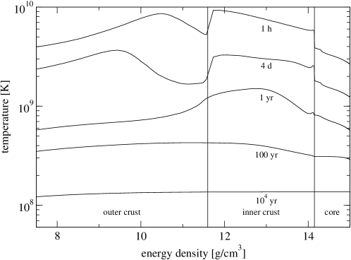
Figure 1: The thermal evolution of our neutron star model with $M=1.45\,M_{\odot}$. As is apparent from this graph, the neutron star is nearly isothermal after 100 years (without heat sources).

In order to provide a picture of what is involved, let us list the ingredients going into this calculation (for a detailed discussion we refer the reader to Ho et al. Ho et al. (2012)). The total heat capacity $C$ is the sum of the partial heat capacities. In the core, these are due to neutrons, protons, electrons and muons whereas in the crust there are contributions from free neutrons, ions and electrons van Riper (1991); Ho et al. (2012).

The neutrino emissivity $\epsilon_{\nu}$ has several contributors as well and must be treated differently in the core and in the crust. In the core, we account for two classes of neutrino emission processes. First, we have the so-called modified Urca processes; we consider both the neutron and the proton branch. The direct Urca process, however, does not contribute since it occurs only at densities higher than those reached by the stellar model we consider here, for which the central density is $\rho_{c}=1\times 10^{15}\,\mathrm{g}\,\mathrm{cm^{-3}}$. Second, we consider bremsstrahlung in which neutrino-antineutrino pairs are produced. In particular, we use emissivities due to neutron-neutron, neutron-proton and proton-proton scattering. The emissivities we use were calculated by Yakovlev et al. Yakovlev et al. (1999a) and Page et al. Page et al. (2004). In the crust, bremsstrahlung is still an important process and we consider electron-nucleon, neutron-neutron and neutron-nucleon scattering. Additionally, we consider the two processes of plasmon decay and electron-positron pair annihilation which could both in principle occur in the core but are much more efficient in low density regions like the crust. We take the emissivities for these processes from Yakovlev et al. Yakovlev et al. (1999b); Yakovlev et al. (2001). For the thermal conductivity of the core, we sum the contributions due to neutrons, electrons and muons Flowers and Itoh (1979, 1981). We take the results of Baiko et al. Baiko et al. (2001) for the neutron thermal conductivity and the results of Shternin & Yakovlev Shternin and Yakovlev (2007) for the electron and muon thermal conductivities. For the crust, we use conduct08 con , which implements the latest advances in calculating thermal conductivities Potekhin et al. (1999); Cassisi et al. (2007); Chugunov and Haensel (2007).

The outer layers — the envelope — of the crust serve as a heat blanket and can support large temperature gradients near the surface of the star Gudmundsson et al. (1982). The relationship between the temperature at the bottom of the envelope $T_{\text{env}}$ and the effective temperature of the photosphere $T_{s}$ depends on the composition of the envelope. We consider envelopes consisting of either iron or light elements and use relations between $T_{\text{env}}$ and $T_{s}$ given by Potekhin et al. Potekhin et al. (2003).

As is apparent from Figure 1, the core of the neutron star cools more quickly than the crust in the very early stages of its life. This is due to stronger neutrino emission in the core and hence the crust is generally hotter than the core. In these very early stages, thermal conductivity does not play a major role in the cooling evolution and the cooling of the core and the crust can be considered more or less decoupled; this leads to the rather big jumps in temperature at the crust-core transition, see Figure 1. The jump between the outer and inner crust is due to the neutron drip. After about one year or so, the star has cooled considerably, so that the cooling mechanisms become less efficient and conductivity will smooth the temperature profile throughout the star, finally bringing it into an isothermal state after about 100 years.

II.4 Crust Formation

As one of our aims is to study shear modes associated with the crust elasticity, we have to specify the region in which the crust may sustain shear stresses. That is, we need to quantify the solid region. The standard idealised model for the crust of a neutron star is a one-component plasma, in which ions of charge $Ze$, number density $n$ and temperature $T$ are free to move. The thermodynamics of such a plasma can be described by the dimensionless Coulomb coupling parameter

$$\Gamma=\frac{(Ze)^{2}}{akT},$$ (12)

where $a=(4\pi n/3)^{-1/3}$ denotes the inter-ion spacing and $k$ is the Boltzmann constant. Calculations by Farouki & Hamaguchi Farouki and Hamaguchi (1993) show that the crust crystallises as $\Gamma$ increases (due to cooling) above $\Gamma_{m}\approx 173$. The DH crust EoS (see Section II.2) we are using provides us with all parameters required to quantify the crust freezing. Given the temperature profiles from our thermal evolution we calculate $\Gamma$ and assume the crust to be elastic in the region in which $\Gamma\geq\Gamma_{m}$. The quantity $\Gamma_{m}$ is associated with uncertainties of a few percent; a slightly different value will affect the thickness of the crust and thereby the frequencies of the shear modes. Similar to the choice of the EoS, we do not further investigate these effects in this study and take the value of $\Gamma_{m}=173$ as given. It can easily be adjusted once more accurate data are available.

In Figure 2, we show how the crust region evolves as the star cools. The crust of the neutron star stays liquid for a bit more than a day; then the crust starts to crystallize at the core-crust interface. Within the first three years the crust gains quickly in width up to about 580m. After about hundred years without any significant further crystallisation, the temperature has dropped below the melting temperature also in the outer layers of the crust and the elastic crust eventually extends nearly to the surface of the star.

Figure 2: The formation of the solid crust over time. We show only the outer layer of our model star. The area where the crust is crystallised is shaded in grey; this region is calculated using a sharp threshold of $\Gamma>173$ (see text).

II.5 Perturbations

Our model accounts for several “restoring forces” expected to be present in a real neutron star, each of which results in a certain, more or less distinct class of modes in the stellar spectrum. The model considered here obviously has the standard $f$-mode (due to the presence of the star’s surface) and acoustic $p$-modes, restored by the pressure. In addition we have composition gradients (leading to composition $g$-modes), a finite temperature (thermal $g$-modes), an elastic crust ($s$-modes) and density discontinuities ($i$-modes). In this section we discuss how the relevant physics enters the perturbation equations.

Before we describe the additional physics, we briefly mention basic definitions. We define the Lagragian displacement vector $\xi^{a}$ to be

$$\xi^{t} =0,$$ (13)

$$\xi^{r} =r^{l}e^{-\lambda/2}\frac{W}{r}P_{l}e^{i\omega t},$$ (14)

$$\xi^{\theta} =-r^{l}\frac{V}{r^{2}}\frac{\mathop{}\!\mathrm{d}P_{l}}{\mathop{}\!\mathrm{d}\theta}e^{i\omega t},$$ (15)

$$\xi^{\phi} =0,$$ (16)

where $W$ and $V$ are functions of $r$ and $P_{l}$ are the Legendre polynomials which account for the angular dependence. The velocity perturbation is then given by

$$\delta u^{a}=q^{a}_{b}\left(u^{c}\nabla_{c}\xi^{b}-\xi^{c}\nabla_{c}u^{b}\right)+\frac{1}{2}u^{a}u^{b}u^{c}h_{bc},$$ (17)

with the projection tensor $q^{ab}=g^{ab}+u^{a}u^{b}$ and $h_{ab}$ the perturbed metric as given later (see Equation (30)).

II.5.1 Stratification

Let us first consider the effects of internal stratification on a given perturbed fluid element. As the fluid moves, weak interaction processes try to adjust the composition to the surrounding matter and restore $\beta$-equilibrium. However, as Reisenegger & Goldreich Reisenegger and Goldreich (1992) have argued, the timescale of the relevant weak interaction processes is much longer than the typical oscillation period and thus perturbed fluid elements are not able to equilibrate during one oscillation. In fact, it is usually appropriate to assume that the composition of a perturbed fluid element is frozen. This means that the adiabatic index $\gamma$ of the perturbed fluid is

$$\gamma=\frac{\rho+p}{p}\left(\frac{\partial p}{\partial\rho}\right)_{n,S},$$ (18)

where $S$ is the entropy per baryon. We will refer to this as the slow reaction limit.

In order to understand the different classes of $g$-modes, it is useful to introduce the Schwarzschild discriminant

$$A=\frac{dp}{dr}-\frac{\gamma p}{\rho+p}\frac{d\rho}{dr}=\left(1-\frac{\gamma}{\gamma_{0}}\right)\frac{dp}{dr},$$ (19)

which determines the stability of a pulsating star against convection Detweiler and Ipser (1973). Stability requires that $A\geq 0$ throughout the star. For our particular EoS this condition holds as we have $\gamma\geq\gamma_{0}$ everywhere. Note that we have used Equation (9) in order to achieve the last equality in Equation (19). Composition $g$-modes arise as the buoyancy associated with $A$ provides a restoring force for small fluid-element deviations from equilibrium.

It may, of course, be the case that the dynamics is much slower than the weak interactions. In the limit of fast reactions the interactions are sufficiently fast to fully adjust the perturbed fluid element’s composition such that it stays in $\beta$-equilibrium at all times. Such a star is called barotropic and the adiabatic indices, $\gamma$ and $\gamma_{0}$, then coincide. As a consequence, the Schwarzschild discriminant vanishes, $A=0$. In this case, perturbed fluid elements are not affected by buoyancy and the $g$-modes due to stratification are absent from the stellar spectrum.

II.5.2 Thermal Pressure

Acting in a fashion similar to that of composition gradients, the presence of a finite temperature leads to a thermal pressure that influences the fluid dynamics. This effect can be important in young neutron stars. Since our EoS models zero temperature physics, we will account for thermal effects by adding the thermal pressure of a Fermi liquid of the form Prakash et al. (1997)

$$p_{th}^{\text{x}}(n_{\text{x}},T)=\frac{\pi^{2}}{6}n_{\text{x}}kT\frac{kT}{E_{F}^{\text{x}}}$$ (20)

to the pressure at zero temperature. Here, $n_{\text{x}}$ is the number density of the relevant species, x=n, p, e and $\mu$ for neutrons, protons, electrons and muons, respectively, $k$ is the Boltzmann constant and $E_{F}^{\text{x}}$ is the Fermi energy of the given species. Note that, in our case $kT/E_{F}^{\text{x}}\ll 1$ throughout most of the star (as our thermal evolutions begin at $kT\approx 1$ MeV), whereas, e.g., Lattimer et al. (1985) consider the thermal pressure when $kT\gtrsim 1$ MeV. As the electrons are relativistic, their Fermi energy is much higher than that of protons or neutrons and as a result their contribution to the thermal pressure is much lower in comparison (the situation is different when the core is considered superfluid and the thermal pressure of protons and neutrons is suppressed—the electron thermal pressure will dominate then). Hence, we will only account for thermal pressure due to neutrons and protons. The non-relativistic nucleon Fermi energy is given by $E_{F}^{\text{x}}=p_{F\text{x}}^{2}/2m^{*}_{\text{x}}$ with $p_{F\text{x}}=\hbar k_{F}^{\text{x}}$ and $k_{F}^{\text{x}}=\left(3\pi^{2}n_{\text{x}}\right)^{1/3}$ and $m^{*}_{\text{x}}$ being the Landau effective mass of the corresponding species (for simplicity, taken to be constant in the following) Chamel and Haensel (2006). Since the EoS gives us information about the composition of the neutron star core, we have all the information we need to account for the thermal pressure due to neutrons and protons, and the total pressure $p$ becomes

$$p=p_{0}(\rho,x_{\text{p}})+\sum_{\text{x}=\text{n},\text{p}}p_{th}^{\text{x}}(n_{\text{x}},T),$$ (21)

where $p_{0}$ is the pressure of the zero temperature EoS described in Section II.2 and $x_{\text{p}}=n_{\text{p}}/n_{\text{b}}$ is the proton fraction ($n_{\text{b}}=n_{\text{n}}+n_{\text{p}}$ is the baryon number density). In order to see how the thermal pressure enters the perturbation equations, we have to calculate the perturbed pressure. Since we are assuming the composition to be frozen we have $\Delta x_{\text{p}}=0$, where $\Delta$ represents a Lagrangian perturbation. The perturbed pressure then is

$$\Delta p=\left(\frac{\partial p_{0}}{\partial\rho}\right)_{x_{\mathrm{p}}}\Delta\rho+\left(\frac{\partial p_{th}^{\text{n}}}{\partial n_{\mathrm{n}}}\right)_{T}\Delta n_{\mathrm{n}}+\left(\frac{\partial p_{th}^{\text{n}}}{\partial T}\right)_{n_{\text{n}}}\Delta T+\left(\frac{\partial p_{th}^{\text{p}}}{\partial n_{\mathrm{p}}}\right)_{T}\Delta n_{\mathrm{p}}+\left(\frac{\partial p_{th}^{\text{p}}}{\partial T}\right)_{n_{\text{p}}}\Delta T.\\$$ (22)

It is, of course, the case that the (cold) energy density $\rho$ is a function of the baryon density. Furthermore, keeping in mind that the composition is frozen and therefore protons and neutrons are conserved separately, it follows Andersson et al. (2002) that

$$\frac{\Delta n_{\mathrm{n}}}{n_{\mathrm{n}}}=\frac{\Delta n_{\mathrm{p}}}{n_{\mathrm{p}}}=\frac{\Delta n_{\text{b}}}{n_{\text{b}}}$$ (23)

since both species are comoving, too. We assume adiabatic oscillations, $\Delta S=0$, which allows us to replace the temperature perturbation, $\Delta T$. The total entropy per baryon, $S$, is given by $S=S_{\text{n}}+S_{\text{p}}$ with Prakash et al. (1987)

$$S_{\text{x}}=\frac{\pi^{2}}{2}\frac{T}{T_{F}^{\text{x}}},$$ (24)

where the Fermi temperature, $T_{F}^{\text{x}}=E_{F}^{\text{x}}/k$, is a function of the number density only, $T_{F}^{\text{x}}=T_{F}^{\text{x}}(n_{\text{x}})$. For simplicity, we assume that the effective mass of both neutrons and protons are identical, $m^{*}_{\text{n}}=m^{*}_{\text{p}}=m^{*}$. Adiabaticity then implies the simple relation

$$\frac{\Delta T}{T}=\frac{2}{3}\frac{\Delta n_{\text{x}}}{n_{\text{x}}}\quad\text{ for }\text{x}=\text{n},\text{p},\text{b}$$ (25)

where we have used Equation (23). From the thermal pressure given by Equation (20), it is easy to show that

$$\left(\frac{\partial p_{th}^{\text{x}}}{\partial T}\right)_{n_{\text{x}}}=\frac{6n_{\text{x}}}{T}\left(\frac{\partial p_{th}^{\text{x}}}{\partial n_{\text{x}}}\right)_{T}.$$ (26)

Using Equations (23), (25) and (26) we can eliminate $\Delta n_{\mathrm{n}}$, $\Delta n_{\mathrm{p}}$ and $\Delta T$ from the perturbed pressure given in Equation (22) in favour of $\Delta n_{\text{b}}$ and arrive at

$$\Delta p=\left[\gamma p_{0}+5n_{\mathrm{n}}\left(\frac{\partial p_{th}^{\text{n}}}{\partial n_{\mathrm{n}}}\right)_{T}+5n_{\mathrm{p}}\left(\frac{\partial p_{th}^{\text{p}}}{\partial n_{\mathrm{p}}}\right)_{T}\right]\frac{\Delta n_{\text{b}}}{n_{\text{b}}},$$ (27)

where we made use of the thermodynamic relation (for $\Delta T=0$)

$$\Delta\rho=\frac{\rho+p}{n_{\text{b}}}\Delta n_{\text{b}}$$ (28)

and the definition of $\gamma$ (see Equation (18)). This provides us with a straightforward way to incorporate the thermal pressure in the perturbation problem. In our simulations, we account for the individual thermal pressures of neutrons and protons in the core. In the crust, there are free neutrons as well as ions present. For simplicity, we assume all baryons contribute as a single Fermi liquid. This is a simplification which in essence implies a maximal thermal component of the pressure. This assumption will be relaxed in future work using the results of, e.g., Lattimer et al. (1985).

II.5.3 The Crust Elasticity

It is not quite as straightforward to account for the elasticity of the star’s crust, at least not in general. The approximation that the star is a perfect fluid has to be abandoned as soon as the solid crust forms, i.e. in the very early stages of a neutron star’s life. The elastic crust supports shear stresses which by definition do not exist in a perfect fluid. To account for such stresses, we have to introduce off-diagonal terms in the stress-energy tensor. However, as we are assuming the background to be in a relaxed, unstrained state, these alterations only appear in the perturbed stress-energy tensor.

Following Penner et al. (2011), the shear strain tensor is given by

$$\delta s_{a}^{b}=\frac{1}{2}\left(\perp^{c}_{a}\perp^{db}-\frac{1}{3}\perp_{a}^{b}\perp^{cd}\right)\Delta g_{cd}.$$ (29)

We will express the metric perturbations in the well-known Regge-Wheeler gauge Regge and Wheeler (1957). This means that the components of the Eulerian perturbations of metric take the form

$$\delta g_{ab}=h_{ab}=-\begin{pmatrix}e^{\nu}r^{l}H_{0}(r)&r^{l+1}\dot{H}_{1}(r)&0&0\\ r^{l+1}\dot{H}_{1}(r)&e^{\lambda}r^{l}H_{2}(r)&0&0\\ 0&0&r^{l+2}K(r)&0\\ 0&0&0&r^{l+2}\sin^{2}\theta K(r)\end{pmatrix}P_{l}(\cos\theta)e^{i\omega t},$$ (30)

where $P_{l}(\cos\theta)$ are the Legendre polynomials and dots denote time derivatives. In the case of a fluid source we have $H_{2}=H_{0}$. The shear associated with the perturbations enters the stress-energy tensor via the anisotropic stress tensor

$$\delta\pi_{a}^{b}=-2\check{\mu}\delta s_{a}^{b},$$ (31)

where $\check{\mu}$ is the shear modulus. We have assumed a Hooke-like relationship between the shear strain and stress. The total perturbed stress-energy tensor then takes the form

$$\delta T_{ab}^{\text{tot}}=\delta T_{ab}+\delta\pi_{ab},$$ (32)

which leads to significant alterations of the perturbation equations compared to the perfect fluid case. In order to deal with this, we define two new variables related to the traction. The radial traction, $T_{1}$, and the tangential traction, $T_{2}$, are defined by

$$T_{1}=\delta\pi_{r}^{r}\quad\text{and}\quad T_{2}=\delta\pi_{r}^{\theta}.$$ (33)

Both variables vanish in the perfect fluid case (as $\check{\mu}\to 0$). However, we will soon see that they are crucial in the implementation of the junction conditions at the crustal interfaces. The complete set of equations governing the perturbations in the elastic crust are lengthy and do not provide deeper insight into the dynamics. We therefore list them, together with their derivation, in Appendix A and mention only the key features here. The most notable difference between the two problems, key to including the extra elastic dynamical degrees of freedom, is the fact that the the metric perturbations $H_{0}$ and $H_{2}$ are no longer identical. Instead, we have

$$H_{2}=H_{0}+64\pi\check{\mu}V\ ,$$ (34)

where $V$ is related to the tangential displacement (see Equation (13)).

II.5.4 Phase-Transitions

Finally, let us consider possible phase-transitions in the star, which may come with a density discontinuity. Having derived the perturbation equations for the elastic crust, we need to connect the perturbations inside the crust to the perturbations for both the fluid core and the thin fluid ocean. This requires us to apply a set of interface conditions at each phase-transition. These conditions stem from the fact that the intrinsic curvature has to be continuous across the interfaces. This problem has already been analysed in detail Finn (1990); Penner et al. (2011). As our analysis is identical, we will simply state the relevant results here: At both crustal interfaces the continuity of the curvature imposes continuity of the perturbation variables $H_{0}$, $H_{1}$, $K$, $W$ and $T_{2}$. In addition to the rather evident interfaces between the crust and the fluid, we have to pay attention to other possible phase-transitions. As explained in Section II.2, the density profile inside a neutron star need not be continuous; phase-transitions at particular densities may cause density discontinuities. Such discontinuities cause the perturbation quantities to become discontinuous. However, it turns out that, as long as it is only the density that is discontinuous, we arrive at the same jump condition as for the crust-fluid interfaces (apart from the continuity of $T_{2}$ which is trivially given as $T_{2}=0$ in the fluid anyway). Furthermore, the Lagrangian pressure perturbation (the variable $X$, see Section III) is continuous across these interfaces.

III Numerical Strategy

The neutron star mode-problem requires the solution of a set of coupled first order differential equations, and the identification of solutions that represent purely outgoing gravitational waves at spatial infinity. The technical issues associated with this problem have been discussed in detail elsewhere, and the approach we take to solve it is relatively standard Thorne and Campolattaro (1967); Detweiler and Lindblom (1985); Finn (1986). Our numerical strategy is conceptually the same as in several previous studies of polar oscillations, the closest being Lin et al. Lin et al. (2008) where a three-layer star was considered. The essential difference is that the “middle” layer in their study was considered superfluid whereas in our case this layer forms the elastic crust. Nevertheless, we still have to deal with different sets of equations depending on whether a given layer is considered a perfect fluid or elastic and the junction conditions required to connect the layers.

We will outline the general idea for a specific case here and save a more technical description for Appendix C. We split the star into several layers, so that each layer requires one unique set of equations to be solved. Depending on the nature of each given layer, we have a certain number (in our case four or six) of independent variables. We start integrating the differential equations at one edge of the layer and continue to the other end; repeating this procedure with linearly independent initial vectors in order to provide us with a basis that can be used to express the general solution to the problem. After doing this for all different layers in the star, we match the solutions at the interfaces. This leads to the need to solve a linear system for the “amplitudes” of the different solutions. The boundary conditions at the centre and the surface of the star finally determine one (up to amplitude) unique solution in the interior of the star. At the surface, we match the solution to the Zerilli function which is solved for outside the star and then calculate the amplitude of the ingoing wave amplitude at infinity, $A_{\mathrm{in}}$. Whenever this amplitude is zero, we have found a quasinormal mode of the star.

The proposed approach has been used successfully in a number of previous studies Detweiler and Lindblom (1985); Kokkotas and Schutz (1992); Comer et al. (1999), but as soon as we consider low-frequency oscillations we run into numerical difficulties. Undesirable noise in the low frequency part of the spectrum (higher order $g$-modes or thermal $g$-modes of old neutron stars as well as some of the $i$-modes would lie in this regime) prevents us from determining any oscillation modes in this regime. The problem is of purely numerical origin and mainly stems from the algebraic equation used to calculate the perturbation variable $V$ (cf. Equation (A14) in Lindblom and Detweiler (1983)):

$$\omega^{2}\left(\rho+p\right)V=e^{\nu/2}X+\frac{1}{r}p^{\prime}e^{\nu-\lambda/2}W-\frac{1}{2}\left(\rho+p\right)e^{\nu}H_{0},$$ (35)

where

$$X=-\frac{1}{r^{l}}e^{\nu/2}\Delta p.$$ (36)

A Taylor expansion (see Detweiler and Lindblom (1985)) reveals that all perturbation variables appearing in this equation, $H_{0}$, $V$, $W$ and $X$, are of the same order of magnitude near the origin. The same is true for the coefficients on the right-hand side. As we are dealing with low frequencies, $\omega M\approx 0.001$ (say), the left-hand side of this algebraic relation forces the sum of the three terms on the right-hand side to be many orders of magnitude smaller than the sum’s constituents, inevitably leading to numerical cancellation and hence inaccurate results.

This problem has already been addressed by Finn Finn (1986), who proposed a different set of equations for the study of low-frequency modes. His formulation makes use of the Eulerian pressure perturbation rather than the Lagrangian one. Such an implementation improves the accuracy of our results as the effect of the cancellation is not as severe; however, it does not fully satisfy our demands. Instead, we derive a new set of equations where the independent variables are a subset of the ‘fundamental’ variables, namely $H_{1}$, $K$, $V$ and $W$. This formulation does not involve an algebraic equation like Equation (35) and thus the cancellation is avoided. The complete set of perturbation equations we use is given in Appendix B. The price we pay for eliminating the cancellation is the appearance of the derivative $\rho^{\prime}$ in the perturbation equations. Since this quantity is not known during the integration of the TOV equations, we have to calculate it numerically on an uneven grid; even worse, it may not be well-defined everywhere since $\rho(r)$ is not necessarily differentiable (density discontinuities may occur inside the star). We use the method proposed by Sundqvist & Veronis Sundqvist and Veronis (1970) to tackle the former problem. In order to overcome the latter, we only use this set of equations in a region near the origin up to a certain radius $R_{V}$, at which point the magnitude of the variables have changed sufficiently that Equation (35) can be applied without significant loss of accuracy and then switch back to the perfect fluid equations from Detweiler and Lindblom (1985). This encourages a rather large value for $R_{V}$. However, when choosing $R_{V}$, we also have to ensure that there are no discontinuities in $\rho$ inside the interval $[0,R_{V}]$ and furthermore, the calculation of $\rho^{\prime}$ suffers from (small but nevertheless present) numerical errors, which favours a small value for $R_{V}$. In the end, the ‘optimal’ value for $R_{V}$ requires trial and error. In our calculations we find that $R_{V}\approx 5\,\mathrm{km}$ is a good choice as it allows us to reliably extract mode frequencies down to $\approx 18\,\mathrm{Hz}$ (the actual lower limit slightly depends on the problem under consideration, see Section IV). For different values of $R_{V}$, the numerical issues become more severe and in the end the low frequency spectrum is contaminated by noise up to higher frequencies. Further work is needed on this problem.

IV Results

Since the spectrum of a relativistic star is rich, and could be difficult to untangle, we will build our understanding by taking the key bits of physics into account step by step. This will gradually enrich the spectrum with more and more classes of oscillation modes. The natural steps are: (i) taking only composition gradients into account, (ii) switching on temperature using the thermal evolution and (iii) accounting for the crystallisation of the elastic crust. The density jumps, leading to $i$-modes, are built-in to the EoS, so we cannot easily switch them on or off. Hence, these modes will always be present in the star’s spectrum.

Let us briefly comment on the actual implementation of the density discontinuities. By far the easiest way of “implementing” them is to simply have them present in the tabulated EoS; for each discontinuity there are two adjacent rows in the given EoS table with nearly (but not actually) identical values for the pressure but the density changes considerably. A TOV solver with adaptive mesh refinement will then lower the step size around these densities and the background model will have large gradients, $\rho^{\prime}$, at these densities. However, the phase-transitions do not appear as proper discontinuities here. It turns out that this is enough to find the interface modes in the spectrum. We also take a different approach to ensure that every phase-transition is reflected by an actual jump in density in our background model. For this, we modified the tabulated EoS by replacing the two pressure values for each phase-transition in the two adjacent rows by their average value. We also adjusted our TOV solver to ensure that two grid points are placed at each phase-transition; both with the same pressure but with the highest and lowest density of the discontinuitiy interval, respectively. When we compare these two implementations, we find that the frequencies of the interface modes with high frequencies are hardly changed while the interface modes with lower frequencies experience a serious shift.

In our calculations, we have to opt for one of these approaches. While the approach with actual discontinuities in density in the background model has the advantage of having a somewhat nicer numerical solution (there won’t be sharp spikes in the density gradient), it is certainly the case that a phase-transition in an actual neutron star occurs over a small but non-zero distance whereby the “simple implementation” is physically favoured. In our results, we opt for using the EoS with actual discontinuities but we point out that a switch to the other case can be done quickly. Jog & Smith Jog and Smith (1982) argued that a phase transition between two layers occurs over a very narrow pressure range $\Delta p$. Typically, this pressure range $\Delta p$ is about four orders of magnitude smaller than the pressure $p$ at which it occurs: $\Delta p\approx 10^{-4}p$. Hence, the approximation of implementing sharp density jumps is quite a good representation of the nuclear composition in the crust.

As in earlier work Detweiler and Lindblom (1985); Andersson et al. (1995), and since our focus is on oscillations that are slowly damped by gravitational-wave emission, we will not actually calculate the complex frequencies of the quasinormal modes; we ignore the damping of the mode. Instead, we construct the asymptotic amplitude $A_{\text{in}}$ for real-valued frequencies and locate the quasinormal modes by approximating the zeros of this function (essentially resonances in the problem). To visualise the spectrum, we plot the logarithm of the incoming amplitude, $\log|A_{\text{in}}|$, as a function of the frequency (as in Figures 3, 5, 7 and 8); the logarithm turns the zeros into much more visible spikes and an eigenfrequency can be found where this function tends to $-\infty$. The damping times can also be estimated using this procedure Andersson et al. (2002) but we will not do so here. In fact, the damping times of (most of) the modes under consideration are so long, i.e. the imaginary part of $\omega$ is many orders of magnitude smaller than its real part, that a reliable calculation of the damping times would be impossible due to the finite machine precision.

We also comment here on the stability of our numerical procedure. As explained earlier, the calculation of the ingoing wave amplitude is spoilt by noise in the low frequency regime and, in practice, the lower limit for reliably extracting frequencies lies at about $18\,\mathrm{Hz}$. In our simulations, we find that this lower limit gets shifted down to approximately $10\,\mathrm{Hz}$ when we include composition, i.e. when we use $\gamma$ instead of $\gamma_{0}$ in the equations (see next subsection). This gives us a further hint to the origin of the instability in the equations. However, this is not the only crucial point since the noisy behaviour is almost non-existent for polytropic equations of state (which we implemented as a test of the numerics).

IV.1 Composition Gradient

The first step beyond barotropic models involves including the composition gradient. Then we expect to find composition $g$-modes in the spectrum as well as $i$-modes due to the density discontinuities. The high frequency domain will be populated by $f$-modes and $p$-modes but we will not discuss this part of the spectrum much as it is well understood Cowling (1941); Detweiler and Lindblom (1985). Instead, we show the low frequency domain up to $200\,\mathrm{Hz}$ (as well as a zoom in at the lower end of the frequency window) for our neutron star model with zero temperature and without solid crust in Figure 3. This frequency range contains all low frequency modes in the model (above the noise cut-off). For comparison we show the spectrum for both the unstratified star (solid line) and the corresponding stratified star (dashed line). All low-frequency modes in an unstratified star are $i$-modes due to density discontinuities and there is precisely one interface mode associated with each density discontinuity. We order them by frequency and label them as $i_{n}$ ($n\geq 1$), where $i_{1}$ is the interface mode with the highest frequency.

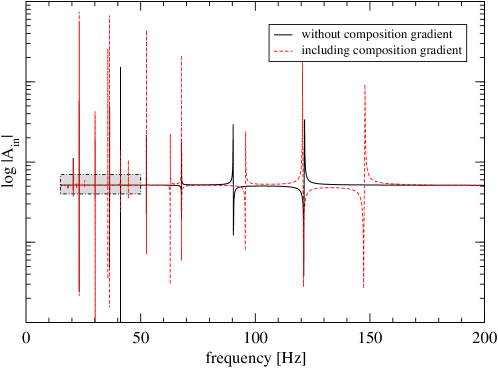
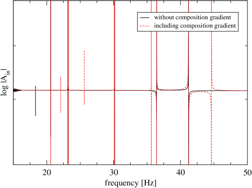
Figure 3: The low frequency spectrum of our neutron star at zero temperature and without a solid crust. The upper panel shows the spectrum up to $200\,\mathrm{Hz}$ whereas the lower panel shows a magnification of the grey shaded area. The solid line shows the spectrum of the pure perfect fluid star, while the dashed line includes composition gradients. All spikes in the solid spectrum are interface modes as there is no composition gradient present; for each of these modes, there is also a mode present in the spectrum of the stratified star (with the exception of the mode at $90.4\,\mathrm{Hz}$; see text). The “new” modes in the dashed spectrum are composition $g$-modes.

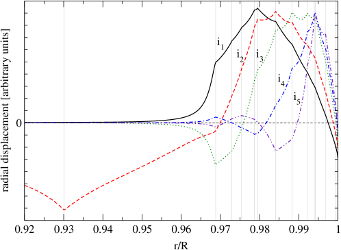
Figure 4: The radial displacement, $\xi^{r}$, for five $i$-modes of the unstratified star. The vertical, grey lines show the location of the different density discontinuities within the star; the interface at $r/R\approx 93\,\%$ is the crust-core interface. The amplitudes of the different modes are scaled so that they are of comparable size. The kinks at the phase-transitions are clearly visible and the displacement nearly vanishes in the core (with the exception of the $i_{2}$-mode which is associated with the crust-core transition). The eigenfunctions are largely unaffected if stratification is switched on (again with the exception of the $i_{2}$-mode which turns into a $g$-mode, see text).

It turns out that the association with interface modes and specific density discontinuities is not unambiguous. The general rule that the radial displacement of an interface mode has its peak amplitude exactly at the corresponding phase-transition does not hold in our case. The eigenfunctions do have their maximum at some phase-transition but we find that several interface modes would belong to the same phase-transition according to this procedure. Likewise, there are discontinuities at which none of the $i$-modes have a maximum. This is the result of the presence of several discontinuities in close vicinity which affect each other. We show the eigenfunctions of five interface modes in Figure 4, where the kinks at the phase-transitions are clearly visible. The modes $i_{4}$ and $i_{5}$ have their strongest peak at the same transition. However, the $i_{1}$ mode has its highest amplitude at a transition where no other interface mode (also the ones which are not shown) has its strongest peak. This suggests that this mode is associated with the transition ${}^{80}\text{Zn}\rightarrow{}^{78}\text{Ni}$. The $i_{2}$-mode apparently has its most prominent peak much deeper in the star and is associated with the artificial discontinuity at the crust-core interface due to the matching of the EoS.

Finn Finn (1987) provides a simple formula to give an estimate for the frequency of an $i$-mode; his calculations show that—in an idealised situation—the frequency of the interface mode is proportional to the relative jump in density, $\Delta\rho/\rho_{+}$, and the distance, $\Delta r$, of the associated phase-transition from the surface of the star. Even though our results qualitatively agree with this estimate, the formula is, unfortunately, not accurate enough to make the exact assocation. Exemplary for the qualitative agreement, we inspect the mode $i_{1}$, which has the highest frequency amongst the interfaces modes in the star. It is due to the transition, which, when compared to the other phase-transition, has the largest relative jump in density of $\Delta\rho/\rho_{+}\approx 4.3\,\%$ and is located rather deep in the star.

All interface modes (except for the one at $90.4\,\mathrm{Hz}$; see discussion below) are still present in the stratified star. However, we find a set of new modes appearing in the spectrum; these are the composition $g$-modes due to the stratification of the core (composition variations in the crust distinguish different layers and so only lead to interface modes associated with transitions from layer to layer). $g$-modes and $i$-modes are easy to distinguish if one examines their eigenfunctions. While the $g$-modes are mainly confined to the core and their radial displacement is a smooth function of the radius, the radial displacement of the $i$-modes nearly vanishes in the core and exhibit kinks at the phase-transitions (cf. Figure 4). In contrast to the $i$-modes, the set of $g$-modes is infinite and we label them as $g_{n}$, where $g_{0}$ is the $g$-mode with the highest frequency and $n$ will correspond to the number of nodes of the radial displacement in the core.

Table 1: Frequencies of the $i$-modes and composition $g$-modes in the stratified, cold star.

Frequency	Mode	Frequency	Mode
[Hz]		[Hz]
147.3	$g_{0}$	30.2	$g_{5}$
121.1	$i_{1}$	30.1	$i_{6}$
95.6	$g_{1}$	25.6	$g_{6}$
67.8	$i_{2}$	23.2	$i_{7}$
62.8	$g_{2}$	23.1	$i_{8}$
52.5	$i_{3}$	22.1	$g_{7}$
44.6	$g_{3}$	20.6	$i_{9}$
41.2	$i_{4}$	19.6	$g_{8}$
36.4	$i_{5}$	18.3	$i_{10}$
35.6	$g_{4}$

Starting from the surface of the star, the 13th jump in density, which is due to the manual matching of the EoS at the crust-core interface, deserves a few more comments since no associated interface mode can be found in the stratified star. When the star is barotropic (not stratified), we find an $i$-mode at $90.4\,\mathrm{Hz}$ associated with this density discontinuity. As this discontinuity lies within (or at least at the edge of) the region where we account for stratification and an interface mode can be understood as a special kind of composition $g$-mode (a sudden change in density indicates a phase-transition and as a result, a perturbed fluid element crossing this interface will experience buoyancy due to the different composition), this $i$-mode loses its character and turns into the lowest order $g$-mode when the star is stratified. To verify this, we ran a series of separate simulations in which we slowly increased the composition gradient via the adiabatic index $\gamma$ from “no stratification” up to “full stratification” (as given in the EoS). The interface mode accordingly increased in frequency and its eigenfunction changed, turning into the $g_{0}$ mode of the stratified star. This example illustrates the close relationship between these two classes of modes.

We list the low frequency modes of the stratified star in Table 1. The spectrum of the barotropic star can be easily extracted from this table by the following procedure: Remove all $g$-modes from this table and add one $i$-mode at $90.4\,\mathrm{Hz}$. The frequencies of the $i$-modes are barely affected by stratification (they vary only by a few tenths of a Hertz).

IV.2 Finite Temperature

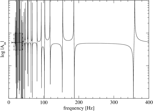
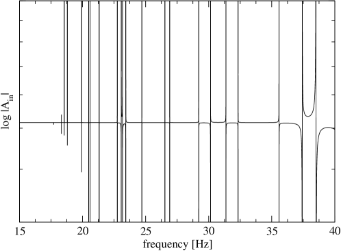
Figure 5: The low frequency spectrum when the star is 3 seconds old; including thermal pressure but without solid crust. The lower panel shows a magnification of the grey shaded area in the upper panel.

The next step is to move away from the assumption that the neutron star is cold. As we have already described, we account for the thermal pressure by adding it to the static pressure of the cold EoS used to determine the background. This leads to the results shown in Figure 5, which shows the low frequency spectrum of an isothermal neutron star with temperature $Te^{\nu}=10^{10}\,\mathrm{K}$ (our initial configuration). In comparison to the result at zero temperature (cf. Figure 3), we find a vastly enriched spectrum. A careful investigation reveals that all composition $g$-modes found in the cold, stratified star are still present in the hot star at only marginally altered frequencies (the difference is generally less than 0.1%, only the high freqency $g$-modes are shifted by up to 4%); likewise their eigenfunctions are unaltered. This is as expected since the composition $g$-modes in our model originate from the composition gradient in the core. The thermal pressure, however, is negligible in the core and hence does not affect the $g$-modes.

For the $i$-modes the situation is somewhat different. We find all interface modes in the hot star, too; however, while the low frequency interface modes maintain their frequency throughout the thermal evolution of the star, four interface modes with high frequencies ($i_{1}$, $i_{2}$, $i_{4}$ and $i_{5}$) have their oscillation period decreased. We are unable to provide a reason as to why this behaviour is observed for precisely these interface modes but not others.

In order to track the evolution of the spectrum as the star ages, we produced a time evolution of the low frequency modes in the following way: We start with the isothermal star at $Te^{\nu}=10^{10}\,\mathrm{K}$, for which the spectrum is that shown in Figure 5, and extract temperature profiles at 120 time steps uniformly distributed on a logarithmic timescale. After extracting the mode frequencies for each of these temperature profiles, we are able to trace the evolution of the oscillation modes over time. This leads to the results shown in Figure 6. All modes exhibit avoided crossings which are easily visible in the high frequency part of the graph; they are also present in the low frequency part, where a higher resolution is necessary to resolve the different modes.

We now find a set of new modes spread over the entire spectrum; these are the thermal $g$-modes. Their frequency decreases as the star cools and after about 100 years nearly all the thermal $g$-modes have frequencies of $18\,\mathrm{Hz}$ or less. This is when the temperature has decreased so far that the thermal pressure is almost negligible and does not affect the frequencies of the $g$- and $i$-modes anymore.

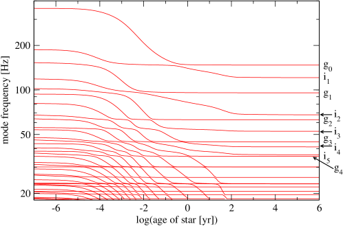
Figure 6: The low-frequency spectrum as the star cools. The thermal $g$-modes quickly decrease in frequency and fall below $18\,\mathrm{Hz}$ after about 100 years. Four of the high frequency interface modes are affected by the thermal pressure ($i_{1}$, $i_{2}$, $i_{4}$ and $i_{5}$). All modes clearly exhibit avoided crossings.

For completeness, we considered the impact of thermal pressure on the fundamental and pressure modes. As an illustration of the results, we show the star’s spectrum after 10 seconds, one month and 100 years in Figure 7. Since the $f$-mode is mainly due to the surface of the star and depends on the average density, it does not change (especially since we do not account for thermal pressure in the background model). The $p$-modes, however, should be affected since the thermal pressure contributes to the restoring force acting on sound waves. In our simulations we observe a slight increase in frequency by up to roughly 10 %, but only for $p$-modes of higher order and only in young, hot neutron stars. As is apparent from Figure 7, after just one month the frequencies of the $p$-modes are only slightly affected by the thermal pressure.

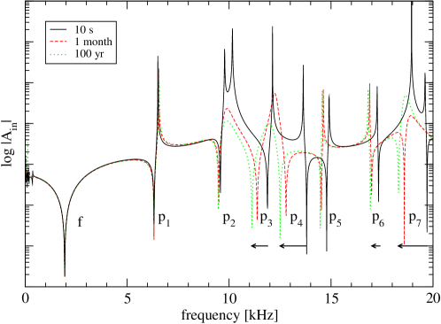
Figure 7: The stellar spectrum up to $20\,\mathrm{kHz}$ for three different temperature profiles. Clearly visible are the $f$-mode and first 7 $p$-modes. Where the frequency of a $p$-mode varies visibly over time, an arrow indicates this change.

IV.3 The Crust Elasticity

Finally, we add the elastic crust to the model. As explained in Section II.4, we define the region in which the crust is solid via the condition $\Gamma>173$ for the Coulomb coupling parameter. As in the previous Section, we start from an isothermal star with $Te^{\nu}=10^{10}\,\mathrm{K}$. At this point, the crust is above its melting temperature and hence liquid; after approximately 1.1 days, the crust starts to crystallise (cf. Figure 2). In Figure 8 we show the spectrum up to $8\,\mathrm{kHz}$ for the neutron star at an age of 100 years, including the thermal pressure and composition gradients. The lower panel in Figure 8 provides a zoom-in at low frequencies. The two most prominent oscillation modes at $1.938\,\mathrm{kHz}$ and $6.315\,\mathrm{kHz}$ are the $f$-mode and the first $p$-mode, respectively; see also Figure 7. As expected, they are unaffected by the presence of the solid crust.

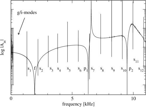
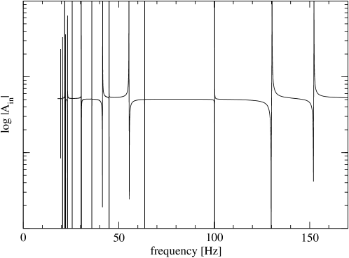
Figure 8: The spectrum of our model star including thermal pressure and an elastic crust, after hundred years of the star’s life. The upper panel shows the high frequency domain, while the lower panel zooms into the grey shaded area at low frequencies to resolve the $g$- and $i$-modes.

The low frequency domain again shows evidence for a large set of oscillation modes. However, only very few modes have maintained their frequency compared to the perfect fluid star. This is not surprising as we have changed the physics of the crust considerably and all the interface modes stem from phase-transitions within the crust. We show the evolution of the low frequency spectrum of the star with elastic crust in the lower panel of Figure 9; for comparison we include the evolution of the star without elastic crust (the dash-dotted lines). Since the crust crystallises only after about 1.1 days, both evolutions coincide in the very early stages of the star’s life. As soon as the crust exhibits elastic parts, the spectra start to diverge from each other. The modes at higher frequencies tend to slightly increase in frequency, whereas the modes at lower frequencies are shifted to lower frequencies.

The threshold between these to different characteristics is the mode at $86.2\,\mathrm{Hz}$ appearing after 1 day (at the time $\log(t/\,\mathrm{yr})=-2.56$ in Figure 9); as soon as the crust solidifies, this mode gets shifted up to $86.7\,\mathrm{Hz}$ and a new mode appears in close vincinity at $82.3\,\mathrm{Hz}$ which cannot be directly linked to any other oscillation mode present in the star that previously had no solid crust. Looking at the eigenfunctions, both modes bear resemblance to each other both in the core and the outer crust, whereas they differ within the inner crust. This is the only new mode appearing in the spectrum (which is accessible to us, i.e. down to $\approx 18\,\mathrm{Hz}$).

Another interesting feature is the disappearance of interface modes in the ageing star. As can be seen from Figure 9, the number of modes in the low frequency spectrum of the star with elastic crust is smaller than if the star was a perfect fluid. The eigenfunctions of the present modes reveal that the elasticity of the crust prevents the large radial displacement at the phase transitions which is characteristic for interface modes: of the few interface modes we can find, all have their maximum radial displacement in the thin fluid ocean, whereas their amplitude is considerably smaller within the elastic crust.

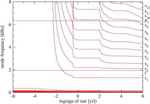
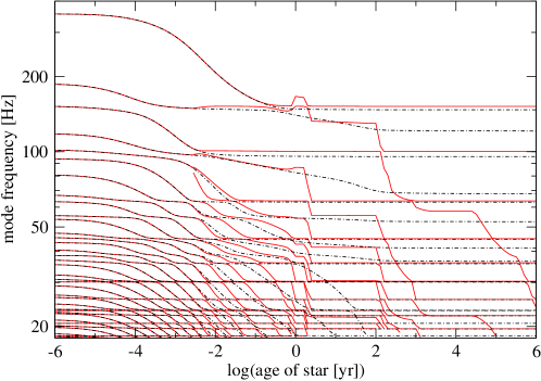
Figure 9: This figure shows how the mode frequencies of the star with elastic crust change as the star cools. Upper panel: Same as Figure 6 but this time for the high frequency part of the spectrum and the model star accounts for the elastic crust. The two modes at constant frequencies, $1.938\,\mathrm{kHz}$ and $6.315\,\mathrm{kHz}$, are the $f$-mode and first $p$-mode, respectively, whose frequencies remain unaffected. The shear modes appear at the top end of the spectrum after about 1.1 days when the crust starts to crystallise. At the bottom of the graph the low frequency $g$-modes and interface modes are visible; see lower panel. Lower panel: A zoom-in at low frequencies in order to resolve the numerous $g$-modes and interface modes. We include the evolution of the low frequency spectrum of the star without elastic crust (dash-dotted lines) for comparison. As the crust of our model star is fluid during its very early stages, the evolutions coincide for about 1.1 days until the crust starts to crystallise. Then the evolution of the low frequency modes is affected by the solid crust, leading to somewhat higher mode frequencies.

In order to investigate this behaviour of the interface modes further, we artificially extend the region in which the crust is elastic towards the surface of the star while keeping the temperature profile of the star fixed at the age of $10^{6}$ years. At first, we extend the crust so that only one phase transition lies within the fluid ocean; in the low frequency spectrum, which we investigate down to frequencies of about $13\,\mathrm{Hz}$, we are able to identify the first 13 $g$-modes and one $i$-mode at about $16.9\,\mathrm{Hz}$; the radial displacement of the $i$-mode is largely confined to the fluid ocean. Next, we gradually increase the thickness of the elastic crust; however, the spectrum does not change significantly as long as the phase transition stays within the fluid ocean. As soon as the elastic crust extends beyond this phase transition, the corresponding $i$-mode starts to decrease in frequency. A further extension of the elastic crust leads to a rapid decrease in frequency (in contrast to the stationary frequency while the phase transition belonged to the fluid ocean, an increase in thickness of the crust by only a few meters results in a decrease of the $i$-modes’s frequency of up to 10 %) and the interface mode soon vanishes from the accessible part of the spectrum. We conclude that the crust elasticity effectively suppresses interface modes. However, the numerical instabilities in the low frequency region prevent us from quantitatively investigating at what frequencies interface modes, which are caused by phase transitions within the elastic crust, can be found.

When we consider higher frequencies, we find several narrow spikes in the spectrum. These belong to the shear modes associated with the solid crust. We list the frequencies of the twelve lowest shear modes for a 100 years old star in Table 2. In Figure 10, we show the radial and transverse displacement of the second shear mode $s_{2}$ (for our neutron star at the age of four months); we denote shear modes by $s_{n}$ where $n$ corresponds to the order of the oscillation mode. Note that we have scaled the transverse displacement, represented by the variable $V$, by a factor of 0.02. That is, the displacement is predominantly transverse. Furthermore, the displacement is strongly confined to the crust (apart from a small, almost constant, radial displacement in the fluid ocean). Both displacement variables fit—to very good precision—one wavelength in radial direction into the elastic crust; however, they are out of phase by approximately $\pi/4$ which indicates an ellipsoidal motion (rather than circular due to the dominance of the transverse displacement) of the “fluid elements” in the crust. The eigenfunctions for the other shear modes show a similar behaviour; higher order shear modes fit more wavelenghts into the elastic crust, in particular, the number of wavelenghts increases by one half per order.

Table 2: Frequencies of the high frequency modes for the neutron star model at the age of hundred years (as shown in Figure 8).

Frequency	Mode
[kHz]
1.304	$s_{1}$
1.938	$f$
2.205	$s_{2}$
3.049	$s_{3}$
3.818	$s_{4}$
4.622	$s_{5}$
5.504	$s_{6}$
6.315	$p_{1}$
6.417	$s_{7}$
7.333	$s_{8}$
8.229	$s_{9}$
9.101	$s_{10}$
9.489	$p_{2}$
9.966	$s_{11}$
10.844	$s_{12}$

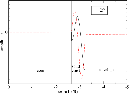
Figure 10: The displacement associated with the second shear mode, $s_{2}$. The star is four months old and its $s_{2}$-mode has a frequency of $2.588\,\,\mathrm{kHz}$.

The frequency of the shear waves deserves a further comment. For reasons that will become clearer later, we again consider our neutron star at the age of four months. It has a solid crust in the region from $R_{cc}=10.94\,\mathrm{km}$ (core-crust interface) to $R_{co}=11.30\,\mathrm{km}$ (crust-ocean interface). As is apparent from Figure 10, the $s_{2}$ mode essentially fits one oscillation into this region, suggesting a wavelength of $\lambda\approx 360\,\mathrm{m}$. This is the same behaviour as observed for axial shear modes Samuelsson and Andersson (2007). Together with the frequency of $2.588\,\mathrm{kHz}$ we infer a wave speed of $c=\lambda f\approx 0.93\times 10^{8}\,\mathrm{cm}/\mathrm{s}$. This is in good agreement with the shear velocity $c_{t}=\sqrt{\hat{\mu}/\rho}$, which varies between $0.98-1.4\times 10^{8}\,\mathrm{cm}/\mathrm{s}$ in the elastic region (as calculated from values provided by the DH EoS). The slight disagreement stems from the fact that the $s_{2}$-mode does not exactly exhibit a full oscillation period. A similar behaviour can of course also be observed in older stars, too. However, as the elastic crust spans a wider region in older stars, the shear speed begins to significantly vary with depth which distorts the neat sinusoidal shape of the eigenfunctions.

In the upper panel of Figure 9 we show how the high frequency part of the spectrum changes with time. We can identify the two frequencies, $1.938\,\mathrm{kHz}$ and $6.315\,\mathrm{kHz}$, which are eigenfrequencies of the star during its entire lifetime (apart from very short periods when a shear mode crosses over and the two modes in question exhibit an avoided crosssing); these are the $f$-mode and the first $p$-mode, respectively. Since the crust does not form until the star is about 1.1 days old, we do not expect to see other modes in the spectrum. As discussed above, we expect the frequency of the shear modes to be determined roughly by the shear speed and the thickness of the elastic crust; when the crust starts to crystallise, the shear modes will have very high frequencies to begin with. Since the crystallised region grows as the star cools, while the shear speed is subject to only small variations, we expect the shear mode frequencies to decrease with time. The described behaviour is clearly visible in the upper panel of Figure 9: The shear modes appear at the top end of the spectrum after about 1.1 days; their frequencies rapidly decrease until the crust reaches a “plateau” after about 1 year. For the next hundred years or so, the crust does not significantly increase in width (cf. Figure 2) and hence the shear modes remain largely unaffected. After this phase the crust gains in width quickly, causing the shear mode frequencies to drop almost discontinuously. After roughly 1000 years, the solid crust has almost reached its final thickness. Thus, the shear modes do not experience a significant change in frequency later.

Our findings for stratified stars with an elastic crust are in agreement with results from McDermott et al. McDermott et al. (1988) who considered a star with an elastic crust in Newtonian theory. Qualitatively, our numerical calculations confirm their spectra; we find the same sets of mode, that is $f$-, $p$-, $g$-, $i$- and $s$-modes. However, while McDermott et al. find two different sets of $g$-modes which they label surface $g$-modes and core $g$-modes, according to the region to which they are mainly confined, our simulations do not reproduce these findings as we do not have a detailed ocean model. Furthermore, the frequencies for the $g$-modes which McDermott et al. find are much lower (below $3\,\mathrm{Hz}$) than in our simulations. This is due to the rather low temperature ($10^{7}\,\mathrm{K}$) used in their calculations. At these temperatures we would expect similar frequencies in our simulations but the numerical procedure does not allow us to investigate the spectrum at such low values.

V Summary and Conclusions

The aim of this paper was to establish a formalism that allows us to study neutron star oscillations in full general relativity, accounting for as much realistic microphysics as possible. So far we extended the standard perfect fluid formalism to account for thermal pressure in the star’s core and derived a new set of equations which govern perturbations in the solid crust. We provided sample results for a particular realistic equation of state. However, our numerical code is generic in the sense that we can easily use a different equation of state straightaway.

We focus our attention on the low-frequency part of the oscillation spectrum (above 15 Hz or so due to computational limitations). In this regime we find a set of interface modes, firstly due to the (artificial) density discontinuity at the crust-core interface and secondly there are interface modes associated with the crust region, due to sharp changes in the low-density equation of state. The composition gradient shifts the frequency of the artificial interface mode to slightly higher frequencies, and we find a set of composition $g$-modes in the low frequency regime. The frequencies of these $g$-modes are slightly lower than literature values from pervious studies—this is because the composition gradient is rather small throughout nearly the entire core; only close to the crust-core transition is the composition gradient reasonably pronounced.

When we account for thermal pressure due to neutrons and protons in the core, we find that a number of thermal $g$-modes enter the low frequency part of the spectrum. Meanwhile, the high frequency interface modes are shifted to even higher frequencies whereas the composition $g$-modes stay unaffected. Tracking the thermal evolution of the neutron star for the first few hundred years, we investigate how the frequencies of the various modes evolve as the star matures through adolescence. After approximately 10 years, all thermal $g$-modes have dropped below $15\,\mathrm{Hz}$ and the thermal effect on the interface modes has almost vanished entirely. During the next 100 years, as the star continues to cool, the frequencies of the interface modes change slightly, finally leaving us with the spectrum of a cold star.

Finally, we considered the crystallization of the crust and investigated the associated changes in the spectrum. From our thermal evolution, we determined the solid region in the outer parts of the star. We quantified how the crust elasticity affects the interface modes associated with the outer layers of the star and we discovered that they are suppressed by shear stress. We discussed how the spectrum is enriched by shear modes. As expected, our results for the shear modes are in good agreement with results from previous work McDermott et al. (1988).

In summary, we have taken the first step towards a comprehensive computational technology to study quasinormal modes of realistic compact stars. We plan to extend the model to account for a multifluid core where the neutrons are superfluid and the protons are superconducting. In doing so we will consider recent equation of state data, in particular concerning the entrainment effect, both in the core and the crust. We will also update the cooling sequence to account for superfluid effects. We expect to report on results in these directions in the not too distant future.

VI Acknowledgements

We are grateful to Ian Hawke and Ian Jones for helpful discussions. CJK acknowledges the use of the IRIDIS High Performance Computing Facility, and associated support services at the University of Southampton, in the completion of this work. WCGH appreciates the use of the computer facilities at the Kavli Institute for Particle Astrophysics and Cosmology. CJK acknowledges financial support from the Engineering and Physical Sciences Research Council (EPSRC) and the School of Mathematics at the University of Southampton. NA and WCGH acknowledge support from the Science and Technology Facilities Council (STFC) in the United Kingdom.

Appendix A Polar Perturbation Equations for the Elastic Crust

The perturbations are governed by the linearised Einstein equations and the conservation laws for the matter:

$$\delta G_{ab}=8\pi\delta T_{ab}\quad\text{and}\quad\delta\left(\nabla_{a}T^{ab}\right)=0,$$ (37)

where $\delta T^{ab}$ denotes the total stress-energy tensor as given in Equation (32). In addition, we have definitions of the two traction variables, $T_{1}$ and $T_{2}$, which in their expanded form read

$$T_{1} =\frac{4}{3}\check{\mu}\left[e^{-\lambda/2}(2l-4)W+2re^{-\lambda/2}\frac{\partial W}{\partial r}+r^{2}(K-H_{2})-l(l+1)V\right],$$ (38)

$$T_{2} =-2\check{\mu}\left[e^{\lambda/2}W-(l-2)V-r\frac{\partial V}{\partial r}\right].$$ (39)

As in the perfect fluid case Lindblom and Detweiler (1983), we use the Lagragian variation of the pressure as an independent variable

$$X=-\frac{1}{r^{l}}e^{\nu/2}\Delta p=\frac{\gamma p}{r^{2}}e^{\nu/2}\left[e^{-\lambda/2}(l+1)W+re^{-\lambda/2}\frac{\partial W}{\partial r}-r^{2}(K+\frac{1}{2}H_{2})+l(l+1)V\right].$$ (40)

For brevity and clarity, we have suppressed the angular dependence in all these relations.

If we define

$$Q=\frac{1}{2}r^{2}e^{-\lambda}\nu^{\prime}\ ,$$ (41)

and

$$m=\frac{1}{2}(l+2)(l-1)\ ,$$ (42)

and make liberal use of Equations (5) - (8), the full set of perturbation equations for the elastic crust reads:

$$\frac{\partial H_{1}}{\partial r} =\left[\frac{1}{2}(\lambda^{\prime}-\nu^{\prime})-\frac{l+1}{r}\right]H_{1}+\frac{e^{\lambda}}{r}\left[H_{2}+K-16\pi(\rho+p)V\right]$$ (43)

$$\frac{\partial K}{\partial r} =\frac{1}{r}H_{2}+\frac{m+1}{r}H_{1}+\left(\frac{1}{2}\nu^{\prime}-\frac{l+1}{r}\right)K-\frac{8\pi(\rho+p)e^{\lambda/2}}{r}W,$$ (44)

$$\frac{\partial H_{0}}{\partial r} =+\frac{\partial K}{\partial r}-re^{-\nu}\omega^{2}H_{1}-\left(\frac{1}{2}\nu^{\prime}+\frac{l-1}{r}\right)H_{0}-\left(\frac{1}{2}\nu^{\prime}+\frac{1}{r}\right)H_{2}+\frac{l}{r}K-\frac{16\pi}{r}T_{2},$$ (45)

$$\frac{\partial W}{\partial r} =-\frac{l+1}{r}W+re^{\lambda/2}\left[\frac{e^{-\nu/2}}{\gamma p}X-\frac{l(l+1)}{r^{2}}V+\frac{1}{2}H_{2}+K\right],$$ (46)

$$\frac{\partial V}{\partial r} =\frac{1}{2\check{\mu}r}T_{2}+\frac{e^{\lambda/2}}{r}W+\frac{2-l}{r}V,$$ (47)

$$\frac{\partial T_{2}}{\partial r} =-\frac{1}{2}re^{\lambda}(\rho+p)H_{0}+re^{\lambda-\nu/2}\left(X-\frac{1}{2r^{2}}e^{\nu/2}T_{1}\right)+\left[\frac{1}{2}(\lambda^{\prime}-\nu^{\prime})-\frac{l+1}{r}\right]T_{2}$$

$$\quad+\left[\frac{4me^{\lambda}\check{\mu}}{r}-e^{\lambda-\nu}r\omega^{2}(\rho+p)\right]V+e^{\lambda/2}p^{\prime}W.$$ (48)

In addition to these six ordinary differential equations (ODEs), we have three algebraic relations:

$$H_{2} =H_{0}+64\pi\check{\mu}V,$$ (49)

$$\left(2M+Q+mr\right)H_{0} =8\pi r^{3}e^{-\nu/2}X-\left[(m+1)Q-\omega^{2}r^{3}e^{-(\lambda+\nu)}\right]H_{1}$$

$$\quad+\left[mr-\omega^{2}r^{3}e^{-\nu}-\frac{e^{\lambda}}{r}Q(2M+Q-r)\right]K$$ (50)

$$\quad+8\pi rT_{1}-16\pi re^{-\lambda}T_{2},$$

$$\frac{2}{3}e^{-\nu/2}\check{\mu}r^{2}X-\frac{1}{4}\gamma pT_{1} =\check{\mu}\gamma p\left[2e^{-\lambda/2}W-r^{2}K+l(l+1)V\right].$$ (51)

The origin of the equations are (for brevity, we denote the components of the Einstein equations with $[ab]$ as a shortcut for $G_{ab}=8\pi T_{ab}$): Equations (43), (44) and (45) are $[t\theta]$, $[tr]$ and $[r\theta]$, respectively; (46) and (47) are due to the definitions of $X$ and $T_{2}$, respectively; (48) is $\delta\left(\nabla_{a}T^{a}_{\theta}\right)=0$; (49) is the difference $[\theta\theta]-[\phi\phi]$; (50) is $[rr]$ and (51) is obtained by removing $\partial_{r}W$ from the definitions of $X$ and $T_{1}$.

Appendix B Low-Frequency Equations

In the low-frequency domain, we need to circumvent numerical difficulties arising from an algebraic equation in the ‘standard formulation’ of the perfect fluid problem. This led us to using $V$ instead of $X$ as an independent variable. The perturbation equations for this set of variables then take the form

$$\frac{\partial H_{1}}{\partial r} =\left[+\frac{1}{2}\left(\lambda^{\prime}-\nu^{\prime}\right)-\frac{l+1}{r}\right]H_{1}+\frac{e^{\lambda}}{r}\left[H_{0}+K-16\pi\left(\rho+p\right)V\right],$$ (52)

$$\frac{\partial K}{\partial r} =\frac{1}{r}H_{0}+\frac{m+1}{r}H_{1}+\left(\frac{1}{2}\nu^{\prime}-\frac{l+1}{r}\right)K-\frac{8\pi\,\left(\rho+p\right)}{r}e^{\lambda/2}W,$$ (53)

$$\frac{\partial W}{\partial r} =-\left(\frac{l+1}{r}+\frac{p^{\prime}}{F}\right)W+re^{\lambda/2}\left[\frac{\rho+p}{F}\left(e^{-\nu}\omega^{2}V+\frac{1}{2}H_{0}\right)-\frac{l(l+1)}{r^{2}}V+\frac{1}{2}H_{0}+K\right],$$ (54)

$$\frac{\partial V}{\partial r} =\left(\frac{p^{\prime}}{F}-\frac{\rho^{\prime}}{\rho+p}+\nu^{\prime}-\frac{l}{r}\right)V+\frac{1}{2\omega^{2}}e^{\nu}\left(\frac{p^{\prime}}{F}-\frac{\rho^{\prime}}{\rho+p}\right)\left(H_{0}+\frac{1}{r}e^{-\lambda/2}\nu^{\prime}W\right)$$

$$\quad+rH_{1}-\frac{1}{r}e^{\lambda/2}W,$$ (55)

where we have introduced the abbreviation

$$F=\gamma p+n_{\mathrm{n}}\frac{\partial p_{th}^{\text{n}}}{\partial n_{\mathrm{n}}}+n_{\mathrm{p}}\frac{\partial p_{th}^{\text{p}}}{\partial n_{\mathrm{p}}}.$$ (56)

The Einstein equations imply the following algebraic relation between the perturbation variables, which we use in order to calculate $H_{0}$:

$$\left[3M-4\pi r^{3}\rho+mr\right]H_{0} =-\left[(m+1)Q-\omega^{2}r^{3}e^{-(\lambda+\nu)}\right]H_{1}$$

$$\quad+\left[mr-\omega^{2}r^{3}e^{-\nu}-\frac{e^{\lambda}}{r}Q(2M+Q-r)\right]K$$ (57)

$$\quad+8\pi e^{\lambda/2}Q(\rho+p)W+8\pi r^{3}e^{-\nu}\omega^{2}\left(\rho+p\right)V,$$

The origin of the equations is basically the same as in previous work, but still deserves a few comments. In order to arrive at our set of equations, we start from the Detweiler & Lindblom set of equations Detweiler and Lindblom (1985). Since the algebraic relation (35) causes numerical problems, we solve it for $X$ and substitute into the other equations. After some algebraic manipulations and making use of the background equations as well as the other perturbation equations, we then arrive at our set of perturbation equations.

Equations (52), (53) and (57) follow from $[t\theta]$, $[tr]$ and $[rr]$ of the perturbed Einstein equations, respectively; (54) is due to the definition of (the no longer appearing) $X$; (55) is $\delta\left(\nabla_{a}T^{a}_{r}\right)=0$ and (35), which has been used as an auxiliary equation only, is $\delta\left(\nabla_{a}T^{a}_{\theta}\right)=0$.

Before we can solve Equation (57) for $H_{0}$, we have to assure that its coefficient is non-singular at any point. This is easy to see, as we have

$$3M=3\int_{0}^{r}4\pi r^{\prime 2}\rho(r^{\prime})dr^{\prime}\geq 3\int_{0}^{r}4\pi r^{\prime 2}\rho(r)dr^{\prime}=4\pi r^{3}\rho,$$ (58)

where we used Equation (5) for the first equality and monotonicity of the density, $\rho(r^{\prime})\geq\rho(r)$ for $r^{\prime}\leq r$, inside the star for the estimate. Thus, the coefficient will be singular only at the origin, $r=0$, where we use a Taylor expansion anyway.

B.1 Behaviour at the Origin

Since the perturbation equations (see Equations (52) - (57)) are singular at the origin due to the use of spherical coordinates, we expand all variables by Taylor series near the origin, $r=0$. For all our perturbation variables $H_{0}$, $H_{1}$, $K$, $V$ and $W$, we use an expansion of the form

$$Q(r)=Q_{0}+\frac{1}{2}r^{2}Q_{2}+\mathcal{O}\left(r^{4}\right).$$ (59)

The field equations imply that the first order corrections vanish. The zeroth order constraints imposed by the perturbation equations are

$$H_{10} =\frac{2lK_{0}+16\pi\left(\rho_{0}+p_{0}\right)W_{0}}{l(l+1)}, V_{0} =-\frac{1}{l}W_{0}, H_{00} =K_{0},$$ (60a)

which demonstrates that, once $K_{0}$ and $W_{0}$ are chosen, the remaining expansion coefficients, $H_{00}$, $H_{10}$ and $V_{0}$ are determined. Here and in the following, we need the expansion coefficients of the background quantities, $\nu$, $\lambda$, $p$ and $\rho$ as well. We expanded them in the same way as specified in Equation (59); their second order coefficients are given by

$$\lambda_{2} =\frac{16}{3}\pi\rho_{0},$$ (61)

$$\nu_{2} =\frac{8}{3}\pi\left(\rho_{0}+3p_{0}\right),$$ (62)

$$p_{2} =-\frac{1}{2}\nu_{2}\left(\rho_{0}+p_{0}\right),$$ (63)

$$\rho_{2} =\frac{p_{2}\left(\rho_{0}+p_{0}\right)}{\gamma p_{0}}.$$ (64)

The second order coefficients of the perturbation variables are then given by the following linear system:

$$-\frac{l+3}{2}H_{12}+\frac{1}{2}K_{2}-8\pi(\rho_{0}+p_{0})V_{2}+\frac{1}{2}H_{02}$$

$$\qquad\qquad\qquad\qquad=\frac{1}{2}(\nu_{2}-\lambda_{2})H_{10}-\lambda_{2}K_{0}+8\pi\left[\rho_{2}+p_{2}+\lambda_{2}(\rho_{0}+p_{0})\right]V_{0},$$ (65a)

$$\frac{m+1}{2}H_{12}-\frac{l+3}{2}K_{2}-4\pi(\rho_{0}+p_{0})W_{2}+\frac{1}{2}H_{02}$$

$$\qquad\qquad\qquad\qquad=-\frac{1}{2}\nu_{2}K_{0}+2\pi\left[2(\rho_{2}+p_{2})+\lambda_{2}(\rho_{0}+p_{0})\right]W_{0},$$ (65b)

$$-(m+1)F_{0}V_{2}-\frac{l+3}{2}F_{0}W_{2}$$

$$\qquad\qquad\qquad\qquad=-\frac{1}{2}\left(3F_{0}+p_{0}+\rho_{0}\right)K_{0}+\left[\frac{m+1}{2}\lambda_{2}F_{0}-lp_{2}-e^{-\nu_{0}}\omega^{2}(\rho_{0}+p_{0})\right]V_{0},$$ (65c)

$$(l+2)V_{2}+W_{2} \qquad\qquad\qquad\qquad=2H_{10}-\frac{e^{\nu_{0}}}{\omega^{2}}\left(\frac{\rho_{2}}{\rho_{0}+p_{0}}-\frac{p_{2}}{F_{0}}\right)K_{0}$$

$$\qquad\qquad\qquad\qquad+\left[\frac{l}{2}\lambda_{2}+2\nu_{2}+\left(2-\frac{le^{\nu_{0}}\nu_{2}}{\omega^{2}}\right)\left(\frac{p_{2}}{F_{0}}-\frac{\rho_{2}}{\rho_{0}+p_{0}}\right)\right]V_{0},$$ (65d)

$$\frac{m}{2}K_{2}-\frac{m}{2}H_{02} \qquad\qquad\qquad\qquad=\left(\frac{m+1}{2}\nu_{2}-\omega^{2}e^{-\nu_{0}}\right)H_{10}+\left(\omega^{2}e^{-\nu_{0}}-\frac{1}{2}\nu_{2}\right)K_{0}$$

$$\qquad\qquad\qquad\qquad-8\pi e^{-\nu_{0}}\omega^{2}(\rho_{0}+p_{0})V_{0}+8\pi p_{2}W_{0}.$$ (65e)

Appendix C Numerical Strategy - General Case

Here, we describe the details of the numerical procedure for the interior solution. In this work, we consider a star with three layers. However, as more physics are taken into account, we will have to slice the neutron star into more layers, each of which extends over a region in which the neutron star matter is homogeneous in the sense that it can be described by the same set of equations. Thus, in anticipation of extending our work to account for superfluidity, where we will certainly have more than three distinct regions within the star, we consider a star with $n$ layers. The same procedure with exactly the same underlying idea and very similar junction conditions has already been explained in great detail for a three-layer star by Lin et al. Lin et al. (2008). Hence, using this $n$-layer description and applying it to our 3-layer star together with the junction conditions from Section II.5 is straightforward.

As an example, consider a neutron star which consists of $n$ layers. The interfaces between the layers, including the center and the surface of the star, are at the radii $0=R_{0}<R_{1}<R_{2}<\cdots<R_{n-1}<R_{n}=R$, where $R$ is the star’s radius. Within each of the different layers, the dynamics and the perturbations, respectively, are governed by a certain set of equations which obviously depends on the nature of the matter within this region. It could be, for instance, a perfect fluid, the elastic crust or a superfluid. We write the equations for layer $i$ as

$$\frac{d{}^{(i)}\mathbf{Y}}{dr}={}^{(i)}\mathbf{Q}\cdot{}^{(i)}\mathbf{Y}\quad\text{for}\quad r\in[R_{i-1},R_{i}],$$ (66)

where ${}^{(i)}\mathbf{Y}=\left(y_{1},\ldots,y_{k_{i}}\right)$ is an abstract vector field with as many entries, say $k_{i}$, as there are independent variables in this layer (in most cases, we have four or six independent variables); ${}^{(i)}\mathbf{Q}={}^{(i)}\mathbf{Q}(r,l,\omega)$ is a $k_{i}\times k_{i}$ matrix (depending also on the background fields, which we have suppressed in this notation). The variables $y_{i}$ are placeholders for the corresponding perturbations variables, like $H_{1}$, $K$, $V$, etc.

Let us now find the general solution in layer $i$. Since we, a priori, do not have any boundary conditions for this layer, we choose some set of values for ${}^{(i)}\mathbf{Y}(R_{i-1})$ and integrate through this layer using Equation (66) until we reach $r=R_{i}$. In order to find the general solution, we repeat this procedure $k_{i}$ times; each time starting with a different set of values for ${}^{(i)}\mathbf{Y}(R_{i-1})$, where all these ‘start vectors’ ought to be linearly independent. This generates $k_{i}$ linearly independent solutions, ${}^{(i)}\mathbf{Y}_{j}(r)$ (with $j=1,\ldots,k_{i}$), and the general solution is a linear combination of these, i.e.

$${}^{(i)}\mathbf{Y}(r)=\sum_{j=1}^{k_{i}}c_{i,j}{}^{(i)}\mathbf{Y}_{j}(r)\quad\text{for}\quad r\in[R_{i-1},R_{i}],$$ (67)

where the coefficients $c_{i,j}$ with $i=1,\ldots,n$ (denoting the layer) and $j=1,\ldots,k_{i}$ (counting the different solutions inside a particular layer) are constants to be determined by interface and boundary conditions. Before we turn to these, we mention some peculiarities while integrating the different layers. Firstly, in some cases it is possible to reduce the computational effort. This happens if some interface condition essentially is a fixed boundary condition for this layer; for instance, a condition could require a variable to vanish at an interface and we will then, of course, apply this condition when choosing the ‘start vectors’, effectively reducing the number of linearly independent solutions. Secondly, the innermost layer (number 1 in our way of counting) needs special treatment as the differential equations, due to the use of spherical coordinates, are most likely singular at the origin, $r=0$. We will therefore expand the solutions at the origin into Taylor series, calculate the Taylor coefficients up to second order and use this expansion up to a small radius at which the ODEs can safely be integrated numerically. Thirdly, the outermost layer $n$ is traditionally integrated from the surface of the star inwards since in most of the cases the Lagrangian pressure perturbation, $X$, is used as a variable which has to vanish at the surface, $X(R)=0$.

Finally, we use the (remaining) interface conditions in order to determine the $\sum_{i}k_{i}$ coefficients $c_{i,j}$. An interface condition connects the solutions between layer $i-1$ and $i$. After fixing the overall normalisation by choosing the value of one of the coefficients $c_{i,j}$, we expect to have $\left(\sum_{i}k_{i}\right)-1$ interface and boundary conditions (less the conditions we used to reduce the computational effort) in order to uniquely determine the solution. The actual interface conditions can take a variety of forms and a general discussion would go well beyond the scope and necessity; therefore, we restrict ourselves to give two common examples only. First, some variables like the metric perturbations are usually continuous across interfaces, i.e. $[H_{1}]_{R_{i}}=0$, whereas other variables simply vanish, i.e. $T_{2}(R_{i}^{-})=0$. The superscript ‘$-$’ in $R_{i}^{-}$ is to denote that we consider the limit of $T_{2}$ at the inner edge of the interface at radius $R_{i}$. These exemplary interface conditions read, respectively

$$\left[H_{1}\right]_{R_{i}} =0\qquad\Leftrightarrow \sum_{j=1}^{k_{i}}c_{i,j}{}^{(i)}H_{1}(R_{i}) =\sum_{j=1}^{k_{i+1}}c_{i+1,j}{}^{(i+1)}H_{1}(R_{i}),$$ (68)

$$T_{2}(R_{i}^{-}) =0\qquad\Leftrightarrow \sum_{j=1}^{k_{i}}c_{i,j}{}^{(i)}T_{2}(R_{i}) =0.$$ (69)

C.1 The Boundary Conditions

The problem we are solving involves matching the solution across different interfaces. The simplest case involves the switch from the equations for low frequencies to the formulation of Detweiler & Lindblom Detweiler and Lindblom (1985). Obviously, all the variables ($H_{0}$, $H_{1}$, $K$, $V$, $W$ and $X$) have to be continuous at the matching point. Since only four of them are independent, we may freely choose four out of these six. It turns out (by inspection) that it is numerically advantageous to use the set of $H_{0}$, $K$, $V$ and $X$ for matching inside the core ($[H_{0}]_{R_{V}}=[K]_{R_{V}}=[V]_{R_{V}}=[X]_{R_{V}}=0$ in short notation). By choosing those four variables, we find that the condition number of the resulting matrix is some orders of magnitude lower than for other combinations. There are also a couple of other sets for which the matrix has a lower condition number but we are unable to reason this behaviour nor are we able to find a pattern. As a rule of thumb, the variables $H_{0}$ and $K$ should be amongst the four chosen ones.

The actual physical interfaces are those which confine the elastic crust. As explained in Section II.5, we have five continuous variables at both sides of the elastic crust, namely $H_{0}$, $H_{1}$, $K$, $W$ and $T_{2}$. We have to use all of them; however, at the core-crust interface, we use the continuity of $T_{2}$, and put it in the form $T_{2}=0$ in order to reduce the number of independent solutions in the crust by one, down to five. Formally, we use $[H_{0}]_{R_{cc}}=[H_{1}]_{R_{cc}}=[K]_{R_{cc}}=[W]_{R_{cc}}=[H_{0}]_{R_{co}}=[H_{1}]_{R_{co}}=[K]_{R_{co}}=[W]_{R_{co}}=0$ and $T_{2}(R_{co}^{-})=0$, where $R_{cc}$ and $R_{co}$ are the radii of the core-crust and the crust-ocean interfaces, respectively.

At the center of the star and at the surface, we impose the boundary conditions from Detweiler & Lindblom Detweiler and Lindblom (1985).

References

- Thorne and Campolattaro (1967) K. S. Thorne and A. Campolattaro, ApJ 149, 591 (1967).
- Lindblom and Detweiler (1983) L. Lindblom and S. L. Detweiler, ApJS 53, 73 (1983).
- Detweiler and Lindblom (1985) S. Detweiler and L. Lindblom, ApJ 292, 12 (1985).
- Kokkotas and Schutz (1992) K. D. Kokkotas and B. F. Schutz, MNRAS 255, 119 (1992).
- Finn (1986) L. S. Finn, MNRAS 222, 393 (1986).
- Finn (1987) L. S. Finn, MNRAS 227, 265 (1987).
- Strohmayer (1993) T. E. Strohmayer, ApJ 417, 273 (1993).
- Miniutti et al. (2003) G. Miniutti, J. A. Pons, E. Berti, L. Gualtieri, and V. Ferrari, MNRAS 338, 389 (2003).
- Schumaker and Thorne (1983) B. L. Schumaker and K. S. Thorne, MNRAS 203, 457 (1983).
- Comer et al. (1999) G. L. Comer, D. Langlois, and L. M. Lin, Phys. Rev. D 60, 104025 (1999).
- Andersson et al. (2002) N. Andersson, G. L. Comer, and D. Langlois, Phys. Rev. D 66, 104002 (2002).
- Lin et al. (2008) L.-M. Lin, N. Andersson, and G. L. Comer, Phys. Rev. D 78, 083008 (2008).
- Sotani et al. (2008) H. Sotani, K. D. Kokkotas, and N. Stergioulas, MNRAS 385, L5 (2008).
- Colaiuda et al. (2009) A. Colaiuda, H. Beyer, and K. D. Kokkotas, MNRAS 396, 1441 (2009).
- Gabler et al. (2012) M. Gabler, P. Cerdá-Durán, N. Stergioulas, J. A. Font, and E. Müller, MNRAS 421, 2054 (2012).
- Gabler et al. (2013) M. Gabler, P. Cerdá-Durán, N. Stergioulas, J. A. Font, and E. Müller, Physical Review Letters 111, 211102 (2013).
- Ferrari et al. (2003) V. Ferrari, G. Miniutti, and J. A. Pons, Classical and Quantum Gravity 20, 841 (2003).
- Andersson (1998) N. Andersson, ApJ 502, 708 (1998).
- Andersson and Kokkotas (2001) N. Andersson and K. D. Kokkotas, International Journal of Modern Physics D 10, 381 (2001).
- Lockitch et al. (2001) K. H. Lockitch, N. Andersson, and J. L. Friedman, Phys. Rev. D 63, 024019 (2001).
- Haskell et al. (2009) B. Haskell, N. Andersson, and A. Passamonti, MNRAS 397, 1464 (2009).
- Watts and Strohmayer (2006) A. L. Watts and T. E. Strohmayer, ApJ 637, L117 (2006).
- Samuelsson and Andersson (2007) L. Samuelsson and N. Andersson, MNRAS 374, 256 (2007).
- Colaiuda and Kokkotas (2011) A. Colaiuda and K. D. Kokkotas, MNRAS 414, 3014 (2011).
- Strohmayer and Mahmoodifar (2014) T. Strohmayer and S. Mahmoodifar, ApJ 784, 72 (2014).
- Andersson et al. (2014) N. Andersson, D. I. Jones, and W. C. G. Ho, MNRAS 442, 1786 (2014).
- Andersson et al. (1999) N. Andersson, K. D. Kokkotas, and N. Stergioulas, ApJ 516, 307 (1999).
- Bondarescu et al. (2007) R. Bondarescu, S. A. Teukolsky, and I. Wasserman, Phys. Rev. D 76, 064019 (2007).
- Abbott et al. (2007) B. Abbott, R. Abbott, R. Adhikari, J. Agresti, P. Ajith, B. Allen, R. Amin, S. B. Anderson, W. G. Anderson, M. Arain, et al., Phys. Rev. D 76, 062003 (2007).
- Abadie et al. (2010) J. Abadie, B. P. Abbott, R. Abbott, M. Abernathy, C. Adams, R. Adhikari, P. Ajith, B. Allen, G. Allen, E. Amador Ceron, et al., ApJ 722, 1504 (2010).
- Abadie et al. (2011a) J. Abadie, B. P. Abbott, R. Abbott, R. Adhikari, P. Ajith, B. Allen, G. Allen, E. Amador Ceron, R. S. Amin, S. B. Anderson, et al., Phys. Rev. D 83, 042001 (2011a).
- Abadie et al. (2011b) J. Abadie, B. P. Abbott, R. Abbott, M. Abernathy, T. Accadia, F. Acernese, C. Adams, R. Adhikari, C. Affeldt, B. Allen, et al., ApJ 734, L35 (2011b).
- Shternin et al. (2011) P. S. Shternin, D. G. Yakovlev, C. O. Heinke, W. C. G. Ho, and D. J. Patnaude, MNRAS 412, L108 (2011).
- Chamel (2008) N. Chamel, MNRAS 388, 737 (2008).
- Andersson et al. (2013) N. Andersson, C. Krüger, G. L. Comer, and L. Samuelsson, Classical and Quantum Gravity 30, 235025 (2013).
- Glampedakis et al. (2011) K. Glampedakis, N. Andersson, and L. Samuelsson, MNRAS 410, 805 (2011).
- Misner et al. (1973) C. W. Misner, K. S. Thorne, and J. A. Wheeler, Gravitation (1973).
- Andersson and Kokkotas (1998) N. Andersson and K. D. Kokkotas, MNRAS 299, 1059 (1998).
- Demorest et al. (2010) P. B. Demorest, T. Pennucci, S. M. Ransom, M. S. E. Roberts, and J. W. T. Hessels, Nature 467, 1081 (2010).
- Antoniadis et al. (2013) J. Antoniadis, P. C. C. Freire, N. Wex, T. M. Tauris, R. S. Lynch, M. H. van Kerkwijk, M. Kramer, C. Bassa, V. S. Dhillon, T. Driebe, et al., Science 340, 448 (2013).
- Steiner et al. (2010) A. W. Steiner, J. M. Lattimer, and E. F. Brown, ApJ 722, 33 (2010).
- Haensel and Potekhin (2004) P. Haensel and A. Y. Potekhin, A&A 428, 191 (2004).
- Ho et al. (2012) W. C. G. Ho, K. Glampedakis, and N. Andersson, MNRAS 422, 2632 (2012), [erratum: 425, 1600 (2012)].
- Burgio et al. (2011) G. F. Burgio, V. Ferrari, L. Gualtieri, and H.-J. Schulze, Phys. Rev. D 84, 044017 (2011).
- Douchin and Haensel (2001) F. Douchin and P. Haensel, A&A 380, 151 (2001).
- Haensel and Pichon (1994) P. Haensel and B. Pichon, A&A 283, 313 (1994), eprint nucl-th/9310003.
- Samuelsson, L. (2003) Samuelsson, L., Ph.D. thesis, Stockholm University (2003).
- van Riper (1991) K. A. van Riper, ApJS 75, 449 (1991).
- Yakovlev et al. (1999a) D. G. Yakovlev, K. P. Levenfish, and Y. A. Shibanov, Physics Uspekhi 42, 737 (1999a).
- Page et al. (2004) D. Page, J. M. Lattimer, M. Prakash, and A. W. Steiner, ApJS 155, 623 (2004).
- Yakovlev et al. (1999b) D. G. Yakovlev, A. D. Kaminker, and K. P. Levenfish, A&A 343, 650 (1999b).
- Yakovlev et al. (2001) D. G. Yakovlev, A. D. Kaminker, O. Y. Gnedin, and P. Haensel, Phys. Rep. 354, 1 (2001).
- Flowers and Itoh (1979) E. Flowers and N. Itoh, ApJ 230, 847 (1979).
- Flowers and Itoh (1981) E. Flowers and N. Itoh, ApJ 250, 750 (1981).
- Baiko et al. (2001) D. A. Baiko, P. Haensel, and D. G. Yakovlev, A&A 374, 151 (2001).
- Shternin and Yakovlev (2007) P. S. Shternin and D. G. Yakovlev, Phys. Rev. D 75, 103004 (2007).
- (57) URL http://www.ioffe.ru/astro/conduct/.
- Potekhin et al. (1999) A. Y. Potekhin, D. A. Baiko, P. Haensel, and D. G. Yakovlev, A&A 346, 345 (1999).
- Cassisi et al. (2007) S. Cassisi, A. Y. Potekhin, A. Pietrinferni, M. Catelan, and M. Salaris, ApJ 661, 1094 (2007).
- Chugunov and Haensel (2007) A. I. Chugunov and P. Haensel, MNRAS 381, 1143 (2007).
- Gudmundsson et al. (1982) E. H. Gudmundsson, C. J. Pethick, and R. I. Epstein, ApJ 259, L19 (1982).
- Potekhin et al. (2003) A. Y. Potekhin, D. G. Yakovlev, G. Chabrier, and O. Y. Gnedin, ApJ 594, 404 (2003).
- Farouki and Hamaguchi (1993) R. T. Farouki and S. Hamaguchi, Phys. Rev. E 47, 4330 (1993).
- Reisenegger and Goldreich (1992) A. Reisenegger and P. Goldreich, ApJ 395, 240 (1992).
- Detweiler and Ipser (1973) S. L. Detweiler and J. R. Ipser, ApJ 185, 685 (1973).
- Prakash et al. (1997) M. Prakash, I. Bombaci, M. Prakash, P. J. Ellis, J. M. Lattimer, and R. Knorren, Phys. Rep. 280, 1 (1997).
- Lattimer et al. (1985) J. M. Lattimer, C. J. Pethick, D. G. Ravenhall, and D. Q. Lamb, Nucl. Phys. A 432, 646 (1985).
- Chamel and Haensel (2006) N. Chamel and P. Haensel, Phys. Rev. C 73, 045802 (2006).
- Prakash et al. (1987) M. Prakash, T. L. Ainsworth, J. P. Blaizot, and H. Wolter, in Windsurfing the Fermi Sea (1987), pp. 357–381.
- Penner et al. (2011) A. J. Penner, N. Andersson, L. Samuelsson, I. Hawke, and D. I. Jones, Phys. Rev. D 84, 103006 (2011).
- Regge and Wheeler (1957) T. Regge and J. A. Wheeler, Physical Review 108, 1063 (1957).
- Finn (1990) L. S. Finn, MNRAS 245, 82 (1990).
- Sundqvist and Veronis (1970) H. Sundqvist and G. Veronis, Tellus 22, 26 (1970).
- Jog and Smith (1982) C. J. Jog and R. A. Smith, ApJ 253, 839 (1982).
- Andersson et al. (1995) N. Andersson, K. D. Kokkotas, and B. F. Schutz, MNRAS 274, 1039 (1995).
- Cowling (1941) T. G. Cowling, MNRAS 101, 367 (1941).
- McDermott et al. (1988) P. N. McDermott, H. M. van Horn, and C. J. Hansen, ApJ 325, 725 (1988).