Exact solution of the optical Bloch equation for the Demkov model

Abstract

An exact analytic solution is presented for coherent resonant excitation of a two-state quantum system driven by a time-dependent pulsed external field described by Demkov model in the presence of dephasing.

I Introduction

Coherent excitation influenced by dephasing processes represents an important topic in quantum mechanics B.Shore ,A-E . Applications of such models are numerious ranging from coherent atomic excitation and quantum information to chemical physics and solid-state physics. Although a significant effort have been devoted for studding the Bloch equations corresponding to specific two-state models, almost all results are related to some asymptotic regimes as weak dephasing, strong coupling or other limits Vitanov . There are very few exact solutions for the Bloch equation. The complexity of this problem is due to the difficulty of deriving an exact solution for third order linear differential equations. In the case of resonant coherent excitation of a two-state system in the presence of dephasing, solution can be found in Kyoseva .

The original Demkov have been introduced in the theory of atomic collisions Demkov .

II Demkov model in the presence of dephasing

Dephasing processes can be incorporated into the description of resonant excitation by including a phenomenological dephasing rate $\Gamma=1/T_{2}$, where $T_{2}$ is the transverse relaxation time, into the Bloch equation,

$$\frac{\text{d}}{\text{d}t}\left[\begin{array}[]{c}u(t)\\ v(t)\\ w(t)\end{array}\right]=\left[\begin{array}[]{ccc}-\Gamma&-\Delta&0\\ \Delta&-\Gamma&-\Omega(t)\\ 0&\Omega(t)&0\end{array}\right]\left[\begin{array}[]{c}u(t)\\ v(t)\\ w(t)\end{array}\right],$$ (1)

where the components of the Bloch vector $\left[u(t),v(t),w(t)\right]^{T}$ are expressed via density matrix elements $\rho_{mn}$ $\left(m,n=1,2\right)$, as follows

$$u(t) = 2\text{Re}\rho_{12}(t)$$ (2)

$$v(t) = 2\text{Im}\rho_{12}(t)$$

$$w(t) = \rho_{22}(t)-\rho_{11}(t)$$

Hereafter the language of laser-atom interactions will be used, although the results apply to any two-state system.The detuning $\Delta=\omega_{0}-\omega$ is the difference between the transition frequency $\omega_{0}$ and the carrier laser frequency $\omega$. The time-varying Rabi frequency $\Omega(t)=\left|dE(t)\right|/\hbar$ describes the laser-atom interaction, where $d$ is the electric dipole moment for the $\psi_{1}\leftrightarrow\psi_{2}$ transition and $E(t)$ is the laser electric field envelope. For the Demkov model we have

$$\Delta =$$ const, (3)

$$\Omega(t) = \Omega_{0}\exp(-\left|t\right|/T),$$

$$\Gamma=\text{const}$$

The constant dephasing rate $\Gamma$ is a positive constant, and $T$ is the characteristic pulse width. The peak Rabi frequency $\Omega_{0}$ will be assumed also positive without loss of generality. For $\Gamma=0$, the Bloch equation Eq.(1) is solved exactly and this solution represents the famous Demkov model Demkov introduced in the theory of atomic collisions.

We shall solve Eq.(1) with the initial conditions corresponding to a system initially in state $\left|1\right\rangle$ i.e. $\rho_{11}(-\infty)=1$ and $\rho_{22}(-\infty)=0.$ This corresponds to

$$u(-\infty)=v(-\infty)=0,\text{ \ \ }w(-\infty)=-1.$$ (4)

Our objective is to find the Bloch vector $\left[u(t),v(t),w(t)\right]^{T}$ and particulary, the population inversion $w(+\infty)$

III Analytic solution of the Demkov model

Due to the specific form of the Demkov model, it is necessary to consider the following two cases: $t\in I_{1}(-\infty;0]$ and $t\in I_{2}[0;+\infty).$ Let us begin with the first of them. Using Eq.(3) from the Bloch system, Eq.(1) we obtain third order differential equation for the population inversion $w,$ which reads.

$$\dddot{w}_{1}-2(T^{-1}-\Gamma)\ddot{w}_{1}+\left[(T^{-1}-\Gamma)^{2}+\Delta^{2}+\Omega_{0}^{2}e^{2t/T}\right]\dot{w}_{1}+$$ (5)

$$\Omega_{0}^{2}(T^{-1}+\Gamma)e^{2t/T}w_{1}=0$$

A subscript ”$1$” in the notation for the population inversion $w_{1}$ indicates that the Eq.(5) above and all formulas hereafter concerns the time interval $t\in I_{1}(-\infty;0].$ The solution of Eq.(5) can be expressed in terms of the generalized hypergeometric function ${}_{1}F_{2}(a_{1};b_{1},b_{2};x).$ Using the transformation

$$x=-\frac{1}{4}(T\ \Omega_{0})^{2}e^{2t/T}$$ (6)

Eq. (5) is transformed to the following form

$$x^{2}w_{1}^{{}^{\prime\prime\prime}}+x(2+T\ \Gamma)w_{1}^{{}^{\prime\prime}}+$$ (7)

$$\left[T\ \Gamma+\frac{(1-T\ \Gamma)^{2}+\Delta^{2}}{4}-x\right]w_{1}^{{}^{\prime}}-\frac{(1+T\ \Gamma)}{2}w_{1}=0$$

Generalized hypergeometric function (GHF) ${}_{1}F_{2}(a_{1};b_{1},b_{2};x)$ satisfies the equation Rainville

$$x^{2}F^{{}^{\prime\prime\prime}}+(b_{1}+b_{2}+1)xF^{{}^{\prime\prime}}+(b_{1}b_{2}-x)F^{{}^{\prime}}-a_{1}F=0,$$ (8)

where $F$ is shortened notation for ${}_{1}F_{2}(a_{1};b_{1},b_{2};x)$. More details regarding basic definitions and formulas for GHF are placed in sec. Appendix. By comparing Eq.(7) and Eq.(8), it is trivial algebra to determine parameters $a_{1};b_{1},b_{2}$ of the GHF

$$b_{1}=\frac{1}{2}+\frac{T\ \Gamma}{2}+i\frac{T\ \Delta}{2},\ b_{2}=(b_{1})^{\ast},\ a_{1}=\text{Re}(b_{1}),$$ (9)

where as usual the notation ”$\ast$” stands for complex conjugation. By reason to simplify the writing of the formulas, hereafter we use

$$\gamma=\frac{T\ \Gamma}{2};\ \delta=\frac{T\ \Delta}{2};\ \omega=\frac{T\ \Omega_{0}}{2}.$$ (10)

Using Eq.(VI) and Eq.(9 ) we obtain the fundamental set of solutions for the problem

$$w_{1}(t)=A_{{}_{-}1}F_{2}\left(\frac{1}{2}+\gamma;\frac{1}{2}+\gamma+i\delta,\frac{1}{2}+\gamma-i\delta;-\omega^{2}e^{2t/T}\right)+B_{-}(-\omega^{2}e^{2t/T})^{\frac{1}{2}-\gamma-i\delta}\!_{1}F_{2}\left(1-i\delta;\frac{3}{2}-\gamma-i\delta,1-2i\delta;-\omega^{2}e^{2t/T}\right)+$$

$$C_{-}(-\omega^{2}e^{2t/T})^{\frac{1}{2}-\gamma+i\delta}\!_{1}F_{2}\left(1+i\delta;1+2i\delta,\frac{3}{2}-\gamma+i\delta;-\omega^{2}e^{2t/T}\right).$$

In Eq.(III) $A_{-},$ $B_{-}$ and $C_{-}$ are integration constants. Next step toward full solution is to determine the integration constants from the initial conditions given by Eq.(4). Using Eq.(1) it is straightforward to rewrite the initial conditions given by Eq.(4) into

$$w_{1}(-\infty)=-1,\ \dot{w}_{1}(-\infty)=0,\ \ddot{w}_{1}(-\infty)=0$$ (11)

From the transformation Eq.(6) we observe that $x(-\infty)=0$ and keep in mind Eq.(44) we will determine the integration constants $A_{-},$ $B_{-}$ and $C_{-}.$ One should note that the exponential factors $(-\omega^{2}e^{2t/T})^{\frac{1}{2}-\gamma-i\delta}$ and $(-\omega^{2}e^{2t/T})^{\frac{1}{2}-\gamma+i\delta}$ oscillate and when $1/2<\gamma$ diverge in the limit $t\rightarrow-\infty$ . In reason to have finite value $w_{1}(-\infty)=-1$ we obtain

$$A_{1}=-1,~{}B_{1}=C_{1}=0.$$ (12)

Finally in the interval $t\in I_{1}(-\infty;0]$ the solution reads

$$w_{1}(t)=-\!_{1}F_{2}\left(\frac{1}{2}+\gamma;\frac{1}{2}+\gamma+i\delta,\frac{1}{2}+\gamma-i\delta;-\omega^{2}e^{2t/T}\right).$$ (13)

Demkov model has a cusp for $\Omega(t)$ at $t=0$. This requires to derive a solution for the interval $t\in I_{2}[0;+\infty)$, where the new initial conditions at $t=0$ are obtained using Eq.(13) and Eq.(45). We should stress that the initial condition given by Eq.(III) has not been derived by taking the second derivative of Eq.(13) at $t=0$. Because of the specific properties of the Demkov model, i.e. cusp of the Rabi frequency $\Omega(t)$ at $t=0,$ one should take the correct derivative of $\Omega(t)$ at $t\rightarrow 0_{+}$ and than using the Bloch equations given by Eq.(1), rigorously to obtain the initial condition Eq.(III).

$$w_{1}(0) = -\!_{1}F_{2}\left(\frac{1}{2}+\gamma;\frac{1}{2}+\gamma+i\delta,\frac{1}{2}+\gamma-i\delta;-\omega^{2}\right)\newline$$

$$\dot{w}_{1}(0) = \frac{2\left(\frac{1}{2}+\gamma\right)\omega^{2}}{T\left[\left(\frac{1}{2}+\gamma\right)^{2}+\delta^{2}\right]}\!_{1}F_{2}\left(\frac{3}{2}+\gamma;\frac{3}{2}+\gamma+i\delta,\frac{3}{2}+\gamma-i\delta;-\omega^{2}\right)$$

$$\ddot{w}_{1}(0) = \frac{4\omega^{2}\left(\frac{1}{2}+\gamma\right)(1-T^{2})}{T^{2}\left[\left(\frac{1}{2}+\gamma\right)^{2}+\delta^{2}\right]}\left[{}_{1}F_{2}\left(\frac{3}{2}+\gamma;\frac{3}{2}+\gamma+i\delta,\frac{3}{2}+\gamma-i\delta;-\omega^{2}\right)\right.+$$

$$\left.\frac{4\omega^{2}\left(\frac{1}{2}+\gamma\right)\left(\frac{3}{2}+\gamma\right)}{T^{2}\left[\left(\frac{1}{2}+\gamma\right)^{2}+\delta^{2}\right]\left[\left(\frac{3}{2}+\gamma\right)^{2}+\delta^{2}\right]}\!_{1}F_{2}\left(\frac{5}{2}+\gamma;\frac{5}{2}+\gamma+i\delta,\frac{5}{2}+\gamma-i\delta;-\omega^{2}\right)\right]$$

By analogy with Eq.(5) for the time interval $t\in I_{2}[0;+\infty)$ we have the following equation for the population inversion

$$\dddot{w}_{2}+2(T^{-1}+\Gamma)\ddot{w}_{2}+\left[(T^{-1}+\Gamma)^{2}+\Delta^{2}+\Omega_{0}^{2}e^{-2t/T}\right]\dot{w}_{2}+$$ (14)

$$\Omega_{0}^{2}(-T^{-1}+\Gamma)e^{-2t/T}w_{2}=0.$$

The solution can again be expressed in term of GHF, after the transformation

$$x=-\frac{1}{4}(T\ \Omega_{0})^{2}e^{-2t/T}.$$

The solution of the equation for the population inversion $w_{2}$ within the time interval $t\in I_{2}[0;+\infty),$ reads

$$w_{2}(t)=A_{+}f_{1}+B_{+}f_{2}+C_{+}f_{3}.$$ (15)

In this equation by reason to simplify some cumbersome formulas, we will denote the three linearly independent solutions of Eq.(15) with $f_{1},$ $f_{2}$ and $f_{3}.$ Adopting the notations introduced by Eq.(10) $f_{1},$ $f_{2}$ and $f_{3}$ are given by

$$f_{1}(t) = \!{}_{1}F_{2}\left(\frac{1}{2}-\gamma;\frac{1}{2}-\gamma-i\delta,\frac{1}{2}-\gamma+i\delta;-\omega^{2}e^{-2t/T}\right)$$ (16a)

$$f_{2}(t) = \!(-\omega^{2}e^{-2t/T})^{\frac{1}{2}+\gamma+i\delta}\!_{1}F_{2}\left(1+i\delta;\frac{3}{2}+\gamma+i\delta,1+2i\delta;-\omega^{2}e^{-2t/T}\right)$$ (16b)

$$f_{3}(t) = (-\omega^{2}e^{-2t/T})^{\frac{1}{2}+\gamma-i\delta}\!_{1}F_{2}\left(1-i\delta;1-2i\delta,\frac{3}{2}+\gamma-i\delta;-\omega^{2}e^{-2t/T}\right)$$ (16c)

We have determined the integration constants $A_{-},$ $B_{-}$ and $C_{-}$ by using the asymptotic behaviours of the exponential factors $(-\omega^{2}e^{2t/T})^{\frac{1}{2}-\gamma-i\delta}$ and $(-\omega^{2}e^{2t/T})^{\frac{1}{2}-\gamma+i\delta}.$ This simple argumentation cannot be used for Eq.(15) and respectively for $A_{+},$ $B_{+}$ and $C_{+}.$ We will determine the integration constants $A_{+},$ $B_{+}$ and $C_{+}$ using the initial conditions at $t=0$, given by Eq.(III). The textbook method requires to write a linear system of equations for the unknown variables $A_{+},$ $B_{+}$ and $C_{+}$. This is done using Eq.(15) by taking $w_{2}(0)$ and the derivatives $\dot{w}_{2}(0)$ and $\ddot{w}_{2}(0).$ After straightforward albeit tedious algebra, using Eq.(LABEL:w1(0)-all) and Eq.(16) we obtain the solution for the integration constants

$$A_{+} = \frac{\left[\begin{array}[]{ccc}w_{1}(0)&f_{2}(0)&f_{3}(0)\\ \dot{w}_{1}(0)&\dot{f}_{2}(0)&\dot{f}_{3}(0)\\ \ddot{w}_{1}(0)&\ddot{f}_{2}(0)&\ddot{f}_{3}(0)\end{array}\right]}{W[f_{1}(0),f_{2}(0),f_{3}(0)]},$$ (17d)

$$B_{+} = \frac{\left[\begin{array}[]{ccc}f_{1}(0)&w_{1}(0)&f_{3}(0)\\ \dot{f}_{1}(0)&\dot{w}_{1}(0)&\dot{f}_{3}(0)\\ \ddot{f}_{1}(0)&\ddot{w}_{1}(0)&\ddot{f}_{3}(0)\end{array}\right]}{W[f_{1}(0),f_{2}(0),f_{3}(0)]},$$ (17h)

$$C_{+} = \frac{\left[\begin{array}[]{ccc}f_{1}(0)&f_{2}(0)&w_{1}(0)\\ \dot{f}_{1}(0)&\dot{f}_{2}(0)&\dot{w}_{1}(0)\\ \ddot{f}_{1}(0)&\ddot{f}_{2}(0)&\ddot{w}_{1}(0)\end{array}\right]}{W[f_{1}(0),f_{2}(0),f_{3}(0)]}.$$ (17l)

The denominator of the expressions for $$A_{+}, B_{+} C_{+} f_{1}, f_{2} f_{3}$$ and is the Wronskian for the three linearly independent solutions and .

Finally, we can write the solution for the Demkov model, bringing together the results from Eqs.(LABEL:w(t)-sol), (12), (15), (16) and (III)

$$w(t)=w_{1}(t)\theta(-t)+w_{2}(t)\theta(t),$$ (18)

where $\theta(t)$ is the Heaviside ”unit step” function. In the very some manner the reader could derive solutions for the coherence components of the Bloch vector $u(t)$ and $v(t).$ Hereafter our main concern will be to investigate the solution for the population inversion $w(t).$

For variate of applications using exact soluble models, the final transition probability expressed via $w(+\infty)$ is more important than time dependent behaviour of the $w(t)$ itself. Having in mind the Demkov model and its solution given by Eq.(18), it is easy to be seen that only the expression for $w_{2}(t)$ is important, when the final transition probability is considered. A closed look to the three linearly independent solutions $f_{1},$ $f_{2}$ and $f_{3}$ reveal that only $f_{1}$ term will survive under the limit $t\rightarrow+\infty$. This is due to the exponential factors $\!(-\omega^{2}e^{-2t/T})^{\frac{1}{2}+\gamma+i\delta}$ and $(-\omega^{2}e^{-2t/T})^{\frac{1}{2}+\gamma-i\delta}$, which tend to zero at $t\rightarrow+\infty$. Using Eq.(44) we arrive at the following expression

$$w(+\infty)=A_{+}.$$ (19)

Although we have closed analytic result for the time dependent $w(t)$ as well as $w(+\infty)$, their complexity impose the use of asymptotic expressions for various limits.

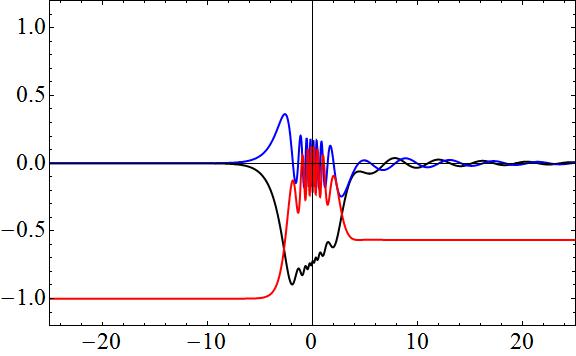
Figure 1: Components of the Block vector. $u(t)$ is plotted with black curve; $v(t)$ is plotted with blue curve; $w(t)$ is plotted with red curve; Model parameters are the following $\delta=1.5$, $\omega_{0}=25$, $\gamma=0.1$

Figure 1 displays the time evolution of the components of the Block vector for a specific values of the parameters.

IV Resonant coherent excitation

Coherent resonant excitation represents an important notion in coherent quantum processes. Besides from the requirement that the frequency of the external field must be equal to the Bohr transition frequency i.e the resonance condition, crucial condition for such processes is also the coherence. Having derived the analytic solutions for the Demkov model in the general case it is instructive to investigate the resonant regime. In this simplified case the Bloch equations take the following form

$$\frac{\text{d}}{\text{d}t}u^{r}(t) = -\Gamma u^{r}(t),$$ (20)

$$\frac{\text{d}}{\text{d}t}\left[\begin{array}[]{c}v^{r}(t)\\ w^{r}(t)\end{array}\right] = \left[\begin{array}[]{cc}-\Gamma&-\Omega(t)\\ \Omega(t)&0\end{array}\right]\left[\begin{array}[]{c}v^{r}(t)\\ w^{r}(t)\end{array}\right].$$ (27)

In the last formula index ”$r$” stands for resonant solution of the Bloch vector. For the resonant case the Bloch equations factorize to a single equation for the coherence $u^{r}(t)$ and a system of two equations for the remaining components of the Bloch vector $\left[v^{r}(t),w^{r}(t)\right]^{T}$. Although the solution of the full Demkov problem requires three linearly independent solutions written in Eqs.(16), the solution for the population inversion $w^{r}(t)$ in the resonant case, is derived from Eq.(27). This system is reducible to a linear differential equation of second order, that posses two linearly independent solutions $f_{1}^{r}(t)$ and $f_{2}^{r}(t)$. Having in mind the symmetry of the GHF and Eqs.(16) it is seen that for the interval $t\in I_{2}[0;+\infty)$, the solutions for the resonant case $\Delta=0,$ are given by

$$f_{1}^{r}(t)=f_{1}(t)|_{\Delta=0};~{}f_{2}^{r}(t)=f_{3}^{r}(t)=f_{2}(t)|_{\Delta=0}=f_{3}(t)|_{\Delta=0}$$

Furthermore the condition $\Delta=0,$ lead to significant simplification of the GHF, which is given by the relation between the GHF and the Bessel function

$$\!{}_{1}F_{2}\left(a;a,b;z\right)=\text{ }_{0}F_{1}\left(\text{ };b;z\right)=\Gamma(b)\left(-z\right)^{\frac{1-b}{2}}J_{b-1}(2\sqrt{-z}).$$ (28)

Using Eq.(LABEL:w(t)-sol) and Eq.(28) we obtain the solution for the resonant Demkov model within the interval $t\in I_{1}(-\infty;0]$

$$w_{1}^{r}(t)=-\ \Gamma\left(\frac{1}{2}+\gamma\right)\left(\omega\!\ e^{t/T}\right)^{\frac{1}{2}+\gamma}J_{-\frac{1}{2}+\gamma}(2\omega\!\ e^{t/T}).$$ (29)

By analogy with the initial conditions Eq.(LABEL:w1(0)-all) for the resonant case we obtain

$$w_{1}^{r}(0) = -\ \Gamma\left(\frac{1}{2}+\gamma\right)\omega\!^{\frac{1}{2}-\gamma}J_{-\frac{1}{2}+\gamma}(2\omega\!\ ),$$ (30)

$$\dot{w}_{1}^{r}(0) = \frac{2}{T\left(\frac{1}{2}+\gamma\right)}\!\Gamma\left(\frac{3}{2}+\gamma\right)\omega\!^{\frac{3}{2}-\gamma}J_{\frac{1}{2}+\gamma}(2\omega\!\ ).$$ (31)

Having in mind the symmetry of the GHF, it is seen that for the interval $t\in I_{2}[0;+\infty)$, the solutions for the resonant case are given by Eqs.(16), where $f_{2}(t)=f_{3}(t),$ under the constrain $\Delta=0.$ For the time interval $t\in I_{2}[0;+\infty)$ we have the following solution of the equation for the population inversion

$$w_{2}^{r}(t)=A_{+}^{r}f_{1}^{r}+B_{+}^{r}f_{2}^{r}.$$ (32)

In Eq.(32) the following notation were used

$$f_{1}^{r}(t) = \ \Gamma\left(\frac{1}{2}-\gamma\right)\left(\omega\!\ e^{-t/T}\right)^{\frac{1}{2}+\gamma}J_{-\frac{1}{2}-\gamma}(2\omega\!\ e^{-t/T}),$$ (33)

$$f_{2}^{r}(t) = \!(-1)^{\frac{1}{2}+\gamma}\!\left(\omega\!\ e^{-t/T}\right)^{\frac{3}{2}+3\gamma}\Gamma\left(\frac{1}{2}-\gamma\right)J_{-\frac{1}{2}-\gamma}(2\omega\!\ e^{-t/T}).$$ (34)

Integration constants $A_{+}^{r}$ and $B_{+}^{r}$ are given by

$$A_{+}^{r} = \frac{\left[\begin{tabular}[]{ll}$w_{1}^{r}(0)$&$f_{2}^{r}(0)$\\ $\dot{w}_{1}^{r}(0)$&$\dot{f}_{2}^{r}(0)$\end{tabular}\right]}{W[f_{1}^{r}(0),f_{2}^{r}(0)]},$$ (37)

$$B_{+}^{r} = \frac{\left[\begin{tabular}[]{ll}$f_{1}^{r}(0)$&$w_{1}^{r}(0)$\\ $\dot{f}_{1}^{r}(0)$&$\dot{w}_{1}^{r}(0)$\end{tabular}\right]}{W[f_{1}^{r}(0),f_{2}^{r}(0)]}.$$ (40)

V Conclusions

VI APPENDIX

For the sake of readers convenience we summarize here some relevant properties of the GHF. Further details can be found in Rainville . Generalized hypergeometric function ${}_{1}F_{2}(a_{1};b_{1},b_{2};x)$ can be introdused as a power series

$${}_{1}F_{2}(a_{1};b_{1},b_{2};x)=\sum_{k=0}^{\infty}\frac{(a_{1})_{k}\ }{(b_{1})_{k}(b_{2})_{k}}\frac{x^{k}}{k!}.$$ (41)

Here it is assumed that none of the bottom parameters $b_{1}$ and $b_{2}$ is a nonpositive integer. As usual $(a_{1})_{k}$ , $(b_{1})_{k}$ and $(b_{2})_{k}$ are Pochhamer symbols i.e. $(\alpha)_{0}=1$ and $(\alpha)_{k}=\alpha(\alpha+1)...(\alpha+k-1)$. Series given by Eq.(41) converges for all finite values of $x$ and defines an entire function. Generalized hypergeometric function ${}_{1}F_{2}(a_{1};b_{1},b_{2};x)$ satisfies the differential equation Eq.(8). When neither $b_{1}$ and $b_{2\text{ }}$are integers, nor the difference $b_{1}-b_{2}$, a fundamental set of solutions of Eq.(8) is given by

$$w(x) = A_{1}F_{2}(a_{1};b_{1},b_{2};x)+$$

$$B\ x^{1-b_{1}}{}_{1}F_{2}(a_{1}+1-b_{1};2-b_{1},b_{2}+1-b_{1};x)+$$

$$C\ x^{1-b_{2}}{}_{1}F_{2}(a_{1}+1-b_{2};b_{1}+1-b_{2},2-b_{2};x)$$

We have, in the neighborhood of the origin three linearly independent solutions. It can be shown Rainville that the Wronskian of these solutions is given by

$$W\left[{}_{1}F_{2}(a_{1};b_{1},b_{2};x);x^{1-b_{1}}{}_{1}F_{2}(a_{1}+1-b_{1};2-b_{1},b_{2}+1-b_{1};x);x^{1-b_{2}}{}_{1}F_{2}(a_{1}+1-b_{2};b_{1}+1-b_{2},2-b_{2};x)\right]$$

$$= (b_{1}-1)(b_{2}-1)(b_{1}-b_{2})x^{-b_{1}-b_{2}-1}$$

Some usefull formulas could be derived from the deffinition Eq.(41). It follows that

$${}_{1}F_{2}(a_{1};b_{1},b_{2};0)=1$$ (44)

The derivatives for the GHF with respect of the independent variable $x$ are given by

$$\frac{d\!\!^{n}}{dx^{n}}\!_{1}F_{2}(a_{1};b_{1},b_{2};x)=\frac{(a_{1})_{n}\ }{(b_{1})_{n}(b_{2})_{n}}\!_{1}F_{2}(a_{1}+n;b_{1}+n,b_{2}+n;x)$$ (45)

Asymtotic expansion of the GHF is given by

$${}_{1}F_{2}(a_{1};b_{1},b_{2};z)\char 126\relax\frac{\Gamma(b_{1})\Gamma(b_{2})\ }{2\sqrt{\pi}\Gamma(a_{1})}(-z)^{\chi}\cos(\pi\chi+2\sqrt{-z})\left(1+O(1/\sqrt{-z})\right)+$$

$$\frac{\Gamma(b_{1})\Gamma(b_{2})\ }{\Gamma(b_{1}-a_{1})\Gamma(b_{2}-a_{1})}(-z)^{-a_{1}}\left(1+O(1/z)\right),\text{ \ }|z|\rightarrow\infty$$

where

$$\chi=\frac{1}{2}\left(a_{1}-b_{1}-b_{2}+\frac{1}{2}\right)$$

References

(1) B. W. Shore, The Theory of Coherent Atomic Excitation
(Wiley, New York, 1990).
(2) L. Allen and J. H. Eberly, Optical Resonance and Two-Level
Atoms (Dover, New York, 1987).
(3) X. Lacour, S. Guerin, L. P. Yatsenko, N. V. Vitanov and H.
R. Jauslin, Uniform analytic description of dephasing effects in two-state
transitions, Phys. Rev. A 75, 033417 (2007).
(4) E. S. Kyoseva and N. V. Vitanov, Resonant excitation
amidst dephasing: An exact analytic solution, Phys. Rev. A 71,
054102 (2005)
(6) E. D. Rainville, Special functions (Macmillan, 1960);
NIST Handbook of Mathematical Functions (CUP, 2010);
http://functions.wolfram.com/HypergeometricFunctions/Hypergeometric1F2/