Containment Control for a Social Network with State-Dependent Connectivity

Abstract

Social interactions influence our thoughts, opinions and actions. In this paper, social interactions are studied within a group of individuals composed of influential social leaders and followers. Each person is assumed to maintain a social state, which can be an emotional state or an opinion. Followers update their social states based on the states of local neighbors, while social leaders maintain a constant desired state. Social interactions are modeled as a general directed graph where each directed edge represents an influence from one person to another. Motivated by the non-local property of fractional-order systems, the social response of individuals in the network are modeled by fractional-order dynamics whose states depend on influences from local neighbors and past experiences. A decentralized influence method is then developed to maintain existing social influence between individuals (i.e., without isolating peers in the group) and to influence the social group to a common desired state (i.e., within a convex hull spanned by social leaders). Mittag-Leffler stability methods are used to prove asymptotic stability of the networked fractional-order system.

, , ,

1 Introduction

Social interactions influence our emotions, opinions, and behaviors. Technological advances in social media provide more rapid, convenient, and widespread communication among individuals, which leads to a more dynamic interaction and influence. For example, recent riots [1] and ultimately revolution [2], have been facilitated through social media technologies such as Facebook, Twitter, YouTube, and BlackBerry Messaging (BBM). Marketing agencies also have begun to take advantage of influence due to social media, especially through the internet. The company Razorfish, for example, works with online peer influencers to transform them into brand advocates through the execution of Social Influence Marketing (SIM) Strategy, which aims to influence marketing primarily through online, small groups, peer pressure, reciprocity or flattery [3].

Various dynamic models have been developed to study the individual’s social behavior, such as the efforts to model the emotional response of different individuals [4, 5, 6]. In [4], the time-variation of emotions between individuals involved in a romantic relationship is described by a dynamic model of love, and in [5] a set of differential equations are developed to model the individual’s happiness in response to exogenous influences. Fractional-order differential equations are a generalization of integer-order differential equations, and they exhibit a non-local integration property where the next state of a system not only depends upon its current state but also upon its historical states starting from the initial time [7]. Motivated by this property, many researchers have explored the use of fractional-order systems as a model for various phenomena in natural and engineered systems. For instance, the works in [4] and [5] were revisited in [8] and [9], where the models of love and happiness were generalized to fractional-order dynamics by taking into account the fact that a person’s emotional response is influenced by past experiences and memories. However, the models developed in [4, 5, 8, 9] only focus on an individual’s emotional response, without considering the interaction with social peers where rapid and widespread influences from social peers can prevail. Other results, such as [10, 11] and the reference therein, studied the interaction of social peers using an opinion dynamics model, and derived conditions under which consensus can be reached. However, agents in [10, 11] only update their opinions by averaging the neighboring agent opinions, without taking into account the influence of agents’ past experience and memory on their decision making.

When making a decision or forming an opinion, individuals tend to communicate with parents, friends, or colleagues and take advice from social peers. Social connections such as friendship, kinship, and other relationships can influence the decisions they make. Some individuals (e.g., parents, teachers, mentors, and celebrities) may exhibit more powerful influences in others’ decision making, and the underlying social network enables the influence to pass from influential individuals to receptive individuals. Containment control is a particular class of consensus problems (see [12, 13] for a comprehensive literature review for consensus problems), in which follower agents are under the influence of leaders through local information exchange in a leader-follower network. In results such as [14, 15, 16, 17], distributed containment control algorithms are developed for agents with integer-order dynamics where the group of followers is driven to a convex hull spanned by multiple leaders’ states under an undirected, directed or switching topology. This paper examines how such methods can be leveraged to manipulate a social network. This work specifically aims to investigate how peer pressure from social leaders affects consensus beliefs (e.g., opinions, emotional states, purchasing decisions, political affiliation, etc.) within a social network, and how an interaction algorithm can be developed such that the group social behavior can be driven to a desired end (i.e., a convex hull spanned by the leaders’ states).

By modeling human emotional response as a fractional-order system, the influence of a person’s emotions within a social network is studied, and emotion synchronization for a group of individuals is achieved in our recent preliminary work [18, 19]. However, the emotion synchronization behavior in [18] only considers an undirected network structure: the one-sided influence of social leaders is not considered. This work aims to investigate how the social beliefs (e.g., emotional response, opinions, etc.) of a group of individuals evolve under the influence of social leaders. Similar to [18], the social group is modeled as a networked fractional-order system, where the social response of each individual is described by fractional-order dynamics whose states depend on influences from social peers, as well as past experiences. Since social leaders are considered, the undirected network topology in [18] is extended to a directed graph, where the directed edges indicate the influence capability between two individuals (e.g., the leaders can influence the followers’ state, but not vice versa). The goal in this work is to develop a decentralized influence algorithm where individuals within a social group update their beliefs by considering beliefs from social peers and the social group achieves a desired common belief (i.e., the social state of the group converges to a convex hull spanned by social leaders). Since an individual generally only considers others’ beliefs as reasonable if their beliefs differ by less than a threshold, social difference is introduced to measure the closeness of the beliefs between individuals. In contrast to the constant weights considered in [14, 15, 16], the social difference is a time-varying weight which depends on individuals’ current states. Moreover, instead of assuming network connectivity (i.e., there always exists a path of influence between any two agents) such as in [14, 15, 16], one main challenge here is to influence the followers’ social states to a desired end by maintaining consistent interaction among social peers and influential leaders (i.e., individuals can always be influenced by social peers, instead of being isolated from the social group) within a time-varying graph. When modeled as a networked fractional-order system, the development of a containment algorithm can be more challenging compared to the integer-order dynamics in [14, 15, 16, 17], which can be considered as a particular case of generalized fractional-order dynamics. The first apparent result that investigated the coordination of networked fractional systems is [20]. However, only linear time-invariant systems are considered in [20], where the interaction between agents is modeled as a link with a constant weight. Due to the time-varying weights considered here, previous stability analysis tools such as examining the eigenvalues of linear time-invariant fractional-order systems (cf. [20, 21, 9]) are not applicable to the time-varying networked fractional-order system in this work. To address these challenges, a decentralized influence function is developed to achieve containment control for the networked fractional-order systems while preserving continued social interaction among individuals. Asymptotic convergence of the social states to the convex hull spanned by leaders’ states in the social network is then analyzed via LaSalles’s invariance theorem [22], convex properties [23] and a Mittag-Leffler stability [24] approach.

2 Preliminaries

Consider a Fractional Order System (FOS)

$${}_{t_{0}}\mathcal{D}_{t}^{\alpha}x\left(t\right)=f\left(t,x\right)$$ (1)

with initial condition $x\left(t_{0}\right)$, where ${}_{t_{0}}\mathcal{D}_{t}^{\alpha}$ denotes the fractional derivative operator with order $\alpha\in(0,1]$ on a time interval $[t_{0},t]$, and $f\left(t,x\right)$ is piecewise continuous in $t$ and locally Lipschitz in $x$. Similar to the exponential function used in solutions of integer-order differential equations, the Mittag-Leffler (M-L) function given by $E_{\alpha,\beta}\left(z\right)=\sum{}_{k=0}^{\infty}\frac{z^{k}}{\Gamma\left(k\alpha+\beta\right)}$, where $\alpha,$ $\beta>0$ and $z\in$ $\mathbb{C}$, is frequently used in solutions of fractional-order systems. Particularly, when $\alpha=\beta=1,$ $E_{1,1}\left(z\right)=e^{x}$ is an exponential function. Stability of the solutions to (1) are defined by the M-L function as follows [24].

Definition 1.

[24] (Mittag-Leffler Stability) The solution of (1) is said to be Mittag-Leffler stable if $\left\|x\left(t\right)\right\|\leq\left\{m\left[x\left(t_{0}\right)\right]E_{\alpha,1}\left(-\lambda\left(t-t_{0}\right)^{\alpha}\right)\right\}^{b},$ where $t_{0}$ is the initial time, $\alpha\in\left(0,1\right),$ $b>0,$ $\lambda>0,$ $m\left(0\right)=0,$ $m\left(x\right)\geq 0,$ $m\left(x\right)$ is locally Lipschitz, and $E_{\alpha,1}$ is defined in $E_{\alpha,\beta}$ with $\beta=1.$

Lyapunov’s direct method is extended to fractional-order systems in the following Lemma to determine Mittag-Leffler stability for the solutions of (1) in [24].

Lemma 2.

[24] Let $x=0$ be an equilibrium point for the fractional order system (1), and $\mathbb{D\subset R}^{n}$ be a domain containing the origin. Let $V\left(t,x\right):\left(0,\infty\right]\times\mathbb{D\rightarrow R}$ be a continuously differentiable function and locally Lipschitz with respect to $x$ such that

$$\sigma_{1}\left(\left\|x\right\|\right) \leq V\left(t,x\right)\leq\sigma_{2}\left(\left\|x\right\|\right),$$

$${}_{0}D_{t}^{\beta}V\left(t,x\right) \leq -\sigma_{3}\left(\left\|x\right\|\right),$$

where $x\in\mathbb{D}$, $\beta\in\left(0,1\right),$ and $\sigma_{i}$ ($i=1,2,3$) are class $\mathcal{K}$ functions. Then $x=0$ is Mittag-Leffler stable, which implies that the equilibrium point of (1) is asymptotically stable.

Definition 3.

[23] For a set of points $X\triangleq\left\{x_{1},\cdots,x_{n}\right\},$ the convex hull $Co\left(X\right)$ is defined as the minimal set containing all points in $X$, satisfying that $Co\left(X\right)\triangleq\left\{\sum\nolimits_{i=1}^{n}\alpha_{i}x_{i}\left|x_{i}\in X,\text{ }\alpha_{i}>0,\mbox{ }\sum\nolimits_{i=1}^{n}\alpha_{i}=1\right.\right\}$.

Graph theory (cf. [26] and [27]) is widely used to represent a networked system. Let $\mathcal{G}=(\mathcal{V},\mathcal{E})$ denote a directed graph, where $\mathcal{V=}\left\{v_{1},\cdots,v_{N}\right\}$ and $\mathcal{E}$ $\subset\mathcal{V\times V}$ denote the set of nodes and the set of edges, respectively. Each edge $\left(v_{i},v_{j}\right)\in\mathcal{E}$ represents the neighborhood of node $i$ and node $j$, which indicates that node $i$ is able to access states of node $j$, but not vice versa. The neighbor set of node $i$ is denoted as $\mathcal{N}_{i}=\left\{v_{j}\text{ }|\text{ }\left(v_{i},v_{j}\right)\in\mathcal{E}\right\}.$ A directed path from node $v_{1}$ to node $v_{k}$ is a sequence of edges $\left(v_{1},v_{2}\right),$ $\left(v_{2},v_{3}\right),\cdots,$ $\left(v_{i},v_{k}\right)$ in the directed graph $\mathcal{G}$. If graph $\mathcal{G}$ contains a directed tree, every node has exactly one parent node except for one node, called the root, and the root has directed paths to every other node in graph $\mathcal{G}$. The adjacency matrix is defined as $A\triangleq\left[a_{ij}\right]\in\mathbb{R}^{N\times N}$ with $a_{ij}>0$ if $\left(v_{i},v_{j}\right)\in\mathcal{E}$, and $a_{ij}=0$ otherwise, where $a_{ij}$ represents a weighting factor for the associated edge $\left(v_{i},v_{j}\right)$. A matrix with positive or zero off-diagonal elements is referred to as a Metzler matrix [28]. The Metzler matrix $L$ for the graph $\mathcal{G}$ is defined as $L\triangleq A-D\in\mathbb{R}^{N\times N}$, where $D\triangleq\left[d_{ij}\right]\in\mathbb{R}^{N\times N}$ is a diagonal matrix with $d_{ii}=\sum\nolimits_{j=1}^{N}a_{ij}.$ To facilitate the following development, a Lemma in [29] is introduced as follows.

Lemma 4.

[29] Consider a linear system $\dot{x}\left(t\right)=A\left(t\right)x\left(t\right),$ and a Lyapunov function $V\left(x\right)=\max\left\{\begin{array}[]{ccc}x_{1},&\cdots,&x_{n}\end{array}\right\}-\min\left\{\begin{array}[]{ccc}x_{1},&\cdots,&x_{n}\end{array}\right\},$ where $x\left(t\right)=\left[x_{1},\ldots,x_{n}\right]^{T}\in$$R^{n}$ is a $n$ dimensional state. If the time-varying matrix $A\left(t\right)\in R^{n\times n}$ is a piecewise continuous function of time with bounded elements, $A\left(t\right)$ is a Metzler matrix with zero row sums, and the time-varying graph corresponding to $A\left(t\right)$ has a spanning tree for all $t\geq 0$, then $\dot{V}\leq 0$ for all $t\geq 0$ and consensus is achieved, i.e., $x_{1}=\cdots=x_{n}$.

3 Problem Formulation

3.1 Individual Social Behavior

Consider a social network composed of $n$ individuals. Each individual $i$ maintains a state $q_{i}(t)\in\mathbb{R}^{d}$ in a social network, which can represent opinions on social events, or human emotional states such as happiness, love, anger or fear. It is assumed that the current state $q_{i}(t)$ of an individual $i$ can be detected from other social neighbors such as close friends or family in the social network. Generally, the opinions or emotional states formed by individuals about social events are not only influenced by the information gathered through communication with their social neighbors, but also depend on their personal experiences. To capture the evolution of individual social states by taking into account not only exogenous influence (e.g., information from friends or family) but also their own character (e.g., past experience, memory), inspired by the works of [8, 9, 10, 11], $q_{i}(t)$ is modeled as the solution to a fractional-order dynamics as

$${}_{0}D_{t}^{\alpha}q_{i}(t)=u_{i}(t),\text{ }i=1,\cdots,n,$$ (2)

where $u_{i}\in\mathbb{R}^{d}$ denotes an influence (i.e., control input) over the social state, and ${}_{0}D_{t}^{\alpha}q_{i}(t)$ is the $\alpha^{th}$ derivative of $q_{i}(t)$ with $\alpha\in(0,1]$.

Note that the model in (2) is a heuristic approximation to a social response, which indicates that a person’s social state has a direct relationship with external influence integrated over the history of a person’s emotional states. On-going efforts by the scientific community are focused on the development of clinically derived models; yet, to date, there is no widely accepted model to describe a person’s social response in a social network.

3.2 Social Interaction

Let $\mathcal{G}\left(t\right)=(\mathcal{V},\mathcal{E}\left(t\right))$ denote a directed graph, where the node set $\mathcal{V}=\left\{1,\cdots,n\right\}$ represents individuals and the edge set $\mathcal{E}\subset\mathcal{V\times V}$ represents the interactions between individuals in a social network. Suppose that there exist $m$ followers $i\in\mathcal{V}_{F}$, $i=1,\cdots,m$, and $n-m$ leaders $j\in\mathcal{V}_{L}$, $j=m+1,\cdots,n$, where $\mathcal{V}_{L}$ and $\mathcal{V}_{F}$ denote the leader and the follower set, respectively, satisfying $\mathcal{V}_{L}\cup\mathcal{V}_{F}=\mathcal{V}$. It is assumed that the leaders’ states $q_{i}\in\mathbb{R}^{d},$ $i\in\mathcal{V}_{L},$ are desired and immutable. For each follower, its state $q_{i}(t),$ $i\in\mathcal{V}_{F},$ evolves according to the dynamics (2) under the influence from both followers and leaders directly or indirectly by the underlying network.

A directed edge $\left(i,j\right)\in\mathcal{E}$ in $\mathcal{G}$ represents the neighborhood of node $i$ and $j$. Each edge $\left(i,j\right)$ is associated with a time-varying weighting factor called the social difference $S_{ij}\in\mathbb{R}^{+},$ which is defined as $S_{ij}=\left\|q_{i}-q_{j}\right\|^{2}.$ Since individuals are assumed that they fail to incorporate the information provided by neighbors whose states are far from their own, the designed social difference $S_{ij}$ aims to capture the closeness of the states between two neighboring nodes $i$ and $j.$ It is also assumed that there exists a threshold $\mathbb{\delta}\in\mathbb{R}^{+}$, and individuals $i$ and $j$ are able to influence each other only when their social difference $S_{ij}\leq\mathbb{\delta}$. In other words, an edge $\left(i,j\right)$ in graph $\mathcal{G}$ does not exist if the social difference $S_{ij}$ is greater than the threshold $\mathbb{\delta}$. The neighbors of individual $i$ in graph $\mathcal{G}$ are defined as $\mathcal{N}_{i}=\left\{j\text{ }|\text{ }S_{ij}\leq\mathbb{\delta}\right\}$, which determines a set of individuals who can influence the social states of individual $i.$ A directed path from node $v_{1}$ to node $v_{k}$ is a sequence of edges $\left(v_{1},v_{2}\right),$ $\left(v_{2},v_{3}\right),\cdots,$ $\left(v_{i},v_{k}\right)$ in the directed graph. If graph $\mathcal{G}$ contains a directed spanning tree, every node has exactly one parent node except for one node, called the root, and the root has directed paths to every other node in graph $\mathcal{G}$.

Assumption 1: For each follower $i\in\mathcal{V}_{F},$ there exists at least one leader that has a directed path to the follower $i$ in the initial graph $\mathcal{G}\left(0\right)$.

Assumption 1 implies that there exists a directed spanning tree for the initial graph $\mathcal{G}\left(0\right)$, where the set of leaders acting as the roots in the directed spanning tree has an influence directly or indirectly on all followers through a series of directed paths in the network. Note that a connected graph (i.e., a directed tree structure) is only assumed in the initial graph, and the controller developed in the subsequent section will preserve the network connectivity to ensure consistent influence between social neighbors.

3.3 Objectives

Let $\mathbf{q}\left(t\right),$ $\mathbf{q}^{F}\left(t\right)$, and $\mathbf{q}^{L}\left(t\right)$ denote the stacked vector of all states $q_{i}\left(t\right),$ $i\in\mathcal{V}$, the followers’ states $q_{i}\left(t\right),$ $i\in\mathcal{V}_{F},$ and the leaders’ states $q_{i}\left(t\right)$, $i\in\mathcal{V}_{L}$, respectively. The convex hull spanned by the states of leaders, and all states (i.e., both leaders and followers), are then represented as $Co\left(\mathbf{q}^{L}\left(t\right)\right)$ and $Co\left(\mathbf{q}\left(t\right)\right),$ respectively. Since the leaders’ states are static, the convex hull $Co\left(\mathbf{q}^{L}\left(t\right)\right)$ is constant, while the convex hull $Co\left(\mathbf{q}\left(t\right)\right)$ is time varying and depends on the states of the followers. After formulating the social network as a networked fractional-order system described by (2), the objective is to regulate the states of followers to a desired region, which is a convex hull spanned by all stationary leaders’ states (i.e., $q_{i}(t)\rightarrow Co\left(\mathcal{V}_{L}\right)$ $\forall i\in\mathcal{V}_{F}$). To ensure that each individual is able to be influenced by social leaders through a path of directed edges by communication with their local neighbors only, another goal is to preserve the network connectivity for the underlying social network (i.e., maintain the social difference $S_{ij}\leq\mathbb{\delta}$ so that peers remain peers) when given an initially connected graph $\mathcal{G}$. Since the systems in (2) along different dimensions are decoupled, for the simplicity of presentation, only a scalar system ($d=1$), that is $q_{i}(t)\in\mathbb{R}$, is considered in the following analysis. However, the results are valid for a $d$ dimensional case by the introduction of the Kronecker product.

4 Distributed Influence Design

The artificial potential field based approach is one of the most widely used methods in the control of multi-agent systems, which consists of an attractive potential encoding the control objective and a repulsive potential representing the motion constraints (cf. [30]). To apply the potential field based approach to a social network problem, inspired by the work of [31] and [32], a decentralized potential function $\varphi_{i}:\mathbb{R}^{d}\rightarrow[0,1]$ $\forall i\in\mathcal{V}_{F}$ is developed to influence the followers’ states to a desired end as

$$\varphi_{i}=\frac{\gamma_{i}}{\left(\gamma_{i}^{k}+\beta_{i}\right)^{1/k}},\text{ }i\in\mathcal{V}_{F}$$ (3)

where $k\in\mathbb{R}^{+}$ is a tuning parameter, $\gamma_{i}:\mathbb{R}^{d}\rightarrow\mathbb{R}^{+}$ is the goal function, and $\beta_{i}:\mathbb{R}^{d}\rightarrow\mathbb{R}^{+}$ is a constraint function. The goal function in (3) is designed as

$$\gamma_{i}=\sum\nolimits_{j\in\mathcal{N}_{i}}\frac{1}{2}\left\|q_{i}-q_{j}\right\|^{2},$$ (4)

which aims to achieve consensus for node $i$ with its neighbors $j\in\mathcal{N}_{i}$. To ensure consistent influence from neighbors (i.e., maintain the social difference $S_{ij}\leq\mathbb{\delta}$), the constraint function in (3) is designed as

$$\beta_{i}=\frac{1}{2}\prod\nolimits_{j\in\mathcal{N}_{i}}b_{ij},$$ (5)

where $b_{ij}=\mathbb{\delta}-S_{ij}\in\mathbb{R}^{+}$. For an existing interaction between individuals $i$ and $j,$ the potential function $\varphi_{i}$ in (3) will approach its maximum whenever the constraint function $\beta_{i}$ decreases to $0$ (i.e., the social difference $S_{ij}$ increases to the threshold of $\mathbb{\delta}$).

Based on the definition of the potential function in (3), the distributed influence algorithm for each follower is designed as

$$u_{i}=-K_{i}\nabla_{q_{i}}\varphi_{i},\text{ }i\in\mathcal{V}_{F}$$ (6)

where $K_{i}$ is a positive gain, and $\nabla_{q_{i}}\varphi_{i}$ denotes the gradient of $\varphi_{i}$ with respect to $q_{i}$. Applying (6) to (2), the closed-loop dynamics of social response for all individuals in a social network can be obtained as

$$\left\{\begin{array}[]{cc}{}_{0}D_{t}^{\alpha}q_{i}(t)=-K_{i}\nabla_{q_{i}}\varphi_{i}&\text{ }i\in\mathcal{V}_{F}\\ {}_{0}D_{t}^{\alpha}q_{i}(t)=0&\text{ }i\in\mathcal{V}_{L}.\end{array}\right.$$ (7)

Since leaders’ states are stationary, the input to leaders in (7) is zero, and $\nabla_{q_{i}}\varphi_{i}$ can be computed as

$$\nabla_{q_{i}}\varphi_{i}=\frac{k\beta_{i}\nabla_{q_{i}}\gamma_{i}-\gamma_{i}\nabla_{q_{i}}\beta_{i}}{k(\gamma_{i}^{k}+\beta_{i})^{\frac{1}{k}+1}}.$$ (8)

From (4) and (5), $\nabla_{q_{i}}\gamma_{i}=\sum\nolimits_{j\in\mathcal{N}_{i}}\left(q_{i}-q_{j}\right)$ and $\nabla_{q_{i}}\beta_{i}=-\sum\nolimits_{j\in\mathcal{N}_{i}}\bar{b}_{ij}\left(q_{i}-q_{j}\right)$ respectively, where $\bar{b}_{ij}\triangleq\prod\nolimits_{l\in\mathcal{N}_{i},l\neq j}b_{il}\in\mathbb{R}^{+}.$ Substituting $\nabla_{q_{i}}\gamma_{i}$ and $\nabla_{q_{i}}\beta_{i}$ into (8), $\nabla_{q_{i}}\varphi_{i}$ is rewritten as

$$\nabla_{q_{i}}\varphi_{i}=\sum\nolimits_{j\in\mathcal{N}_{i}}m_{ij}\left(q_{i}-q_{j}\right),$$ (9)

where

$$m_{ij}=\frac{k\beta_{i}+\bar{b}_{ij}\gamma_{i}}{k(\gamma_{i}^{k}+\beta_{i})^{\frac{1}{k}+1}}$$ (10)

is non-negative, based on the definition of $\gamma_{i}$, $\beta_{i}$, $k$, and $\bar{b}_{ij}$.

5 Convergence Analysis

To show that the followers in the fractional-order network converge to a convex hull spanned by the static leaders’ states, the following analysis is segregated into three proofs. The first proof shows that the existing interaction between individuals is maintained by the influence function designed in (6) (i.e., the social difference $S_{ij}\leq\mathbb{\delta}$ for all time, meaning influential peers remain influential), and thus the connectivity for the social network is preserved. The second proof yields the asymptotic stability for an integer-order representation of the dynamic system in (2), which is then used to establish the asymptotic convergence to the equilibrium set of consensus states for the fractional-order system by using a Mittag-Leffler stability analysis in the third proof.

5.1 Maintenance of Social Influence

If a directed graph $\mathcal{G}\left(t\right)$ does not have a directed spanning tree, there must exist a follower to which all leaders do not have a directed path to influence the follower’s states. Hence, the state of the follower is independent of the influence of leaders, and thus can not converge to the stationary convex hull spanned by leaders. To ensure the continued influence from leaders to all followers, a directed spanning tree structure must be maintained all the time. The following theorem shows that, given an initial graph containing a directed spanning tree assumed in Assumption 1, the tree structure will be preserved under the influence function in (6) (i.e., network connectivity is maintained and social peers do not become isolated from the social group).

Theorem 5.

The influence function in (6) guarantees a directed spanning tree structure in $\mathcal{G}$ for all time.

It is assumed that the initial graph $\mathcal{G}\left(0\right)$ has a directed spanning tree in Assumption 1. If every existing edge in $\mathcal{G}\left(0\right)$ is preserved, the tree structure will also be preserved. Since an individual only considers a local neighbor’s opinion as reasonable when their social difference $S_{ij}\leq\mathbb{\delta}$, peer influence is maintained when each edge $S_{ij}\leq\mathbb{\delta}$ all the time. Consider a state $q_{0}$ for individual $i$, where the interaction between individual $i$ and neighbor $j\in\mathcal{N}_{i}$ satisfies $b_{ij}\left(q_{0},q_{j}\right)=0,$ which indicates that their social difference is too large to influence each others’ opinion, and the associated edge is about to break. From (5), $\beta_{i}=0$ when $b_{ij}=0$, and the navigation function $\varphi_{i}$ achieves its maximum value from (3). Since $\varphi_{i}$ is maximized at $q_{0},$ no open set of initial conditions can be attracted to $q_{0}$ under the negative gradient control law designed in (6). Therefore, the social bond between individual $i$ and $j$ is maintained less than $\delta$ by (6), and the associated edge is also maintained. Repeating this argument for all pairs, every edge in $\mathcal{G}$ is maintained and the directed spanning tree structure is preserved. ∎

5.2 Convergence Analysis

To establish asymptotic convergence to the equilibrium points (i.e., the convex hull $Co\left(\mathbf{q}^{L}\left(t\right)\right)$ for the fractional-order dynamics in (2), an integer-order system $\dot{q}_{i}(t)=u_{i}(t)$ with $\alpha=1$ in (7) is considered first in the following theorem.

Theorem 6.

Consider a network composed of stationary leaders and dynamic followers described by (7). The followers $i\in V_{F}$ asymptotically converge to the equilibrium points (i.e., a convex hull $Co\left(\mathbf{q}^{L}\left(t\right)\right)$ spanned by the leaders states only), if there always exists at least one leader $j\in V_{L}$ that has a directed path to any follower $i$ (i.e., a directed spanning tree is maintained).

This theorem is proven by using LaSalle’s invariance principle and convex properties. Let $V\left(\mathbf{q}\left(t\right)\right)$ be the volume of the convex hull $Co\left(\mathbf{q}\left(t\right)\right)$ formed by all leaders’ and followers’ states. First, we show that there exists a compact set $\Omega$ such that if $q_{i}\left(0\right)\in\Omega$ for $\forall i\in\mathcal{V}$, then $q_{i}\left(t\right)\in\Omega$ for all $t\geq 0$, which implies that $\Omega$ is a positively invariant set. Second, let $E$ be the set of all points in $\Omega$ where $\dot{V}=0$ (i.e., the volume of $Co\left(\mathbf{q}\left(t\right)\right),$ $\mathbf{q}\left(t\right)\in E$, stays constant). It is then shown that $M$ is the largest invariant set, where $M$ is the set of points in the convex hull $Co\left(\mathbf{q}^{L}\left(t\right)\right)$ formed by stationary leaders only.

Substituting (9) into (7) with $\alpha=1$ yields the following closed-loop emotion dynamics

$$\left\{\begin{array}[]{cc}\dot{q}_{i}(t)=-\sum\limits_{j\in\mathcal{N}_{i}}K_{i}m_{ij}\left(q_{i}\left(t\right)-q_{j}\left(t\right)\right)&\text{ }i\in\mathcal{V}_{F}\\ \dot{q}_{j}(t)=0&\text{ }j\in\mathcal{V}_{L},\end{array}\right.$$ (11)

which can be rewritten in a compact form of a time-varying linear system as

$$\mathbf{\dot{q}}\left(t\right)=\left[\begin{array}[]{c}\mathbf{\dot{q}}^{F}\left(t\right)\\ \mathbf{\dot{q}}^{L}\left(t\right)\end{array}\right]=\left[\begin{array}[]{c}\pi\left(t\right)\\ \mathbf{0}_{(n-m)\times n}\end{array}\right]\mathbf{q}\left(t\right),$$ (12)

where $\mathbf{0}_{(n-m)\times n}$ denotes the $\left(n-m\right)\times n$ matrix with all zeros, and the elements of $\pi\left(t\right)\in\mathbb{R}^{m\times n}$ are defined as

$$\pi_{ik}\left(t\right)=\left\{\begin{array}[]{cc}-\sum\limits_{j\in\mathcal{N}_{i}}K_{i}m_{ij}&i=k\\ K_{i}m_{ik}&k\in\mathcal{N}_{i},i\neq k\\ 0,&k\notin\mathcal{N}_{i},i\neq k.\end{array}\right.$$ (13)

Each follower $i\in\mathcal{V}_{F}$ in (11) evolves according to the dynamics:

$$\dot{q}_{i}(t)=-\sum\limits_{j\in\mathcal{N}_{i}}\pi_{ij}\left(t\right)\left(q_{i}\left(t\right)-q_{j}\left(t\right)\right).$$ (14)

To facilitate the analysis, (14) can be written in discrete time as

$$q_{i}(t+1)=\left(1-T\sum\limits_{j\in\mathcal{N}_{i}}\pi_{ij}\right)q_{i}\left(t\right)+T\sum\limits_{j\in\mathcal{N}_{i}}\pi_{ij}q_{j}\left(t\right),$$ (15)

where $T$ is a sufficiently small sampling period. From (15), it is clear that $q_{i}(t+1)$ is a convex combination of its current state $q_{i}\left(t\right)$ and its neighbors’ states $q_{j}\left(t\right)$, $j\in\mathcal{N}_{i}$, which implies that the follower $i$ moves towards the convex hull spanned by itself and its neighborhood set $\mathcal{N}_{i}$. Since the leaders’ states are stationary and the followers’ states are evolving within the convex hull, $V\left(\mathbf{q}\left(t\right)\right)$ is uniformly non-increasing and thus $V\left(\mathbf{q}\left(0\right)\right)$ is the compact set $\Omega$.

The next step is to show that all followers’ states will asymptotically converge to their equilibrium points. To see that the equilibrium points are indeed the stationary convex hull $Co\left(\mathbf{q}^{L}\left(t\right)\right)$, let $q_{i,eq}$ be an equilibrium point for a follower $i\in\mathcal{V}_{F}$. For an equilibrium point, it must have $\dot{q}_{i,eq}=0,$ and (14) can be written as $-\sum_{j\in\mathcal{N}_{i}}\pi_{ij}\left(t\right)\left(q_{i,eq}\left(t\right)-q_{j,eq}\left(t\right)\right)=0$, which yields that

$$q_{i,eq}=\frac{1}{-\pi_{ii}\left(t\right)}\sum_{j\in\mathcal{N}_{i}}\pi_{ij}\left(t\right)q_{j,eq}\left(t\right)$$ (16)

by using (14). Due to the fact that $-\pi_{ii}\left(t\right)=\sum_{j\in\mathcal{N}_{i}}\pi_{ij}\left(t\right)\in\mathbb{R}^{+}$ from (13), (16) indicates that the equilibrium point $q_{i,eq}$ lies in a convex hull spanned by its neighbors’ states (i.e., leaders and/or followers). Since every follower ends up in a convex hull spanned by its neighbors’ states and the leaders’ states are static, every follower will end up in a convex hull spanned by the leaders states only (i.e., $Co\left(\mathbf{q}^{L}\left(t\right)\right)$). Using the fact that $m_{ij}$ is non-negative from (10) and $K_{i}$ is a positive constant gain in (6), $\left[\begin{array}[]{c}\pi\left(t\right)\\ \mathbf{0}_{(n-m)\times n}\end{array}\right]$ in (12) is a Metzler matrix with zero row sums. According to Lemma 4 and following a similar procedure as in [29], the convex hull $Co\left(\mathbf{q}\left(t\right)\right)$ is shrinking (i.e., $\dot{V}\left(\mathbf{q}\left(t\right)\right)<0$), since the difference of the extremes $\max\left\{\begin{array}[]{ccc}x_{1},&\cdots,&x_{n}\end{array}\right\}$ and $\min\left\{\begin{array}[]{ccc}x_{1},&\cdots,&x_{n}\end{array}\right\}$ is decreasing. If all followers states are initially within the convex hull $Co\left(\mathbf{q}^{L}\left(t\right)\right),$ the states will always stay within $Co\left(\mathbf{q}^{L}\left(t\right)\right)$ (i.e., $\dot{V}=0$).

A proof by contradiction can now be used to show that $M$ (i.e., $Co\left(\mathbf{q}^{L}\left(t\right)\right)$) is the largest invariant set. Let $M^{\prime}\supset M$ be a larger invariant set in $E$. Suppose that there is a follower whose state $q_{i}\left(0\right)\notin M$, and $q_{i}\left(0\right)$ is on the boundary of $M^{\prime}.$ Since $M^{\prime}\subset E,$ the volume of the set $M^{\prime}$ stays constant. The only way for the volume of $M^{\prime}$ to stay constant is that $q_{i}\left(0\right)=q_{i}\left(t\right)$ for all $t\geq 0.$ However, for this to happen, we must have $\pi_{ij}\left(t\right)=0$ for $\forall j\in\mathcal{N}_{i}$ from (14), which indicates that the follower $i$ is isolated from the group. This isolation is a contradiction with network connectivity. Hence, $M$ is the largest invariant set. The followers asymptotically converge to the largest invariant set $M$ (i.e., the equilibrium points $Co\left(\mathbf{q}^{L}\left(t\right)\right)$) by using LaSalle’s invariance principle in [22]. ∎ Since asymptotic stability for the integer-order system (11) is established in Theorem 6, a similar proof procedure in our recent work [18] can be followed to prove asymptotic stability for the fractional order system in (7) by using Mittag-Leffler stability analysis and a Converse Lyapunov Theorem.

Theorem 7.

The follower $i\in V_{F}$, with closed-loop fractional-order dynamics in (7) with $\alpha\in(0,1)$, asymptotically converges to the convex hull spanned by stationary leaders if at least one leader $j\in V_{L}$ has a directed path to the follower $i$.

Let $x_{i}\left(t\right)\triangleq q_{i}\left(t\right)-q_{i,eq},$ and $\mathbf{x}^{F}\left(t\right)\triangleq\mathbf{q}^{F}\left(t\right)-\mathbf{q}_{eq}^{F}$, where $\mathbf{q}_{eq}^{F}$ denotes the stacked vector of $q_{i,eq}$. Since the leaders’ states are constant, the closed-loop fractional-order dynamics in (7) can be written in a compact form as

$${}_{0}D_{t}^{\alpha}\mathbf{x}^{F}\left(t\right)=g(\mathbf{x}^{F}),$$ (17)

for all followers where $g(\mathbf{x}^{F})$ is a function of follower states. Since stability of a fractional-order system is defined by Definition 1, and Mittag-Leffler stability implies asymptotic convergence as discussed in [24], the following development aims to show that (17) is Mittag-Leffler stable.

Since asymptotic stability is established in Theorem 6 for the integer-order system of (15), a Converse Lyapunov Theorem, (i.e., Theorem 4.16 in [22]) is invoked to establish that there exists a function $V\left(t,\mathbf{x}^{F}\right):\left(0,\infty\right]\times\mathbb{R}^{m}\mathbb{\rightarrow R}$ and class $\mathcal{K}$ functions $\sigma_{i}$ ($i=1,2,3$) such that

$$\sigma_{1}\left(\left\|\mathbf{x}^{F}\right\|\right)\leq V\left(t,\mathbf{x}^{F}\right)\leq\sigma_{2}\left(\left\|\mathbf{x}^{F}\right\|\right),$$ (18)

$$\dot{V}\leq-\sigma_{3}\left(\left\|\mathbf{x}^{F}\right\|\right).$$ (19)

Let $\beta=1-\alpha\in(0,1)$. From Theorem 8 in [24] and (19), the fractional derivative of $V$ is computed as

$${}_{0}D_{t}^{\beta}V\left(t,\mathbf{x}^{F}\right) = \text{ }_{0}D_{t}^{1-\alpha}V\left(t,\mathbf{x}^{F}\right)=\text{ }_{0}D_{t}^{-\alpha}\dot{V}$$ (20)

$$\leq \text{ }-_{0}D_{t}^{-\alpha}\left(\sigma_{3}\left(\left\|\mathbf{x}^{F}\right\|\right)\right).$$ (21)

From the definition of the fractional integral ${}_{0}D_{t}^{-\alpha}f\left(t\right)=\frac{1}{\Gamma\left(\alpha\right)}\int_{0}^{t}\frac{f\left(\tau\right)}{\left(t-\tau\right)^{1-\alpha}}d\tau$, where $\Gamma\left(\cdot\right)$ denotes the Gamma function [7], it is known that ${}_{0}D_{t}^{-\alpha}\left(\cdot\right)$ is a class $\mathcal{K}$ function, since ${}_{0}D_{t}^{-\alpha}\left(0\right)=0$ and ${}_{0}D_{t}^{-\alpha}\left(\cdot\right)$ is strictly increasing on the domain $\left[0,\infty\right)$. Using the fact that $a_{1}\circ a_{2}$ also belongs to class $\mathcal{K}$, where $a_{1}$ and $a_{2}$ are class $\mathcal{K}$ functions, the term ${}_{0}D_{t}^{-\alpha}\left(\sigma_{3}\left(\left\|\mathbf{x}^{F}\right\|\right)\right)$ in (21) is a class $\mathcal{K}$ function, since both ${}_{0}D_{t}^{-\alpha}\left(\cdot\right)$ and $\sigma_{3}\left(\cdot\right)$ are class $\mathcal{K}$ functions. Thus, the inequality in (21) can be written as

$${}_{0}D_{t}^{\beta}V\left(t,\mathbf{x}^{F}\right)\leq-\sigma_{4}\left(\left\|\mathbf{x}^{F}\right\|\right),$$ (22)

where $\sigma_{4}\left(\left\|\mathbf{x}^{F}\right\|\right)\triangleq$ ${}_{0}D_{t}^{-\alpha}\left(\sigma_{3}\left(\left\|\mathbf{x}^{F}\right\|\right)\right)$ is a class $\mathcal{K}$ function. Applying Lemma 2 to (18) and (22), Mittag-Leffler stability of (17) with $\alpha\in(0,1)$ can be obtained, which implies that the equilibrium points $\mathbf{q}_{eq}^{F}$ for the followers in the closed-loop fractional-order system in (17) are asymptotically stable. ∎

6 Simulations

To illustrate the proposed control algorithms, simulations are performed on a karate club network described in [33]. The karate club network considered in this section consists of 3 social leaders and 7 followers, and is represented as a directed graph in Fig. 1. The solid arrow connecting two individuals in Fig. 1 indicates an established social bond (e.g., friendship) and the directed influence between individuals. Note that the leaders can not be influenced, while the followers can be influenced by social peers as well as social leaders. Based on the topology described in Fig. 1, each individual is randomly assigned a social state (e.g., an opinion on an event or an emotional state such as happiness, fear and anger). Without loss of generality, we assume that the social states of individuals are two dimensional (i.e., $q_{i}(t)\in\mathbb{R}^{2}$). The control law in (6) yields the simulation results shown in Fig. 2, which illustrates that the followers’ states converge to the convex hull formed by the social leaders.

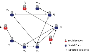
Figure 1: The Zachary’s karate club network is modeled by a directed graph.

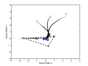
Figure 2: Evolution of social states. The followers’ states converge to the convex hull formed by social leaders, where the the leaders’ social states are denoted as squares, and the followers’ initial and final social states are denoted by circles and dots, respectively.

7 Conclusion

By modeling the group social response as a networked fractional-order system, a decentralized potential field-based influence algorithm is developed in this work to ensure that all individuals’ states achieve consensus asymptotically to a desired convex hull spanned by the stationary leaders’ states, while maintaining consistent influence between individuals (i.e., network connectivity). This work considers individuals whose social response is modeled by a FOS with $\alpha\in(0,1]$. Since some individuals may respond with a more complex dynamic (e.g., $\alpha\in(1,2]$), future efforts will focus on generalizing the development to include networks with heterogeneous members with higher order dynamic response. Future effort will also consider different influence capabilities between individuals. For instance, a person tends to have a larger tolerance for a difference of opinions for a certain social event in a close friend than a loose acquaintance, and thus, can be more easily influenced by the close friend.

References

- [1] P. Bright, “How the London riots showed us two sides of social networking,” Ars Technica, August 10 2011.
- [2] S. Gustin, “Social media sparked, accelerated Egypt’s revolutionary fire,” Wired, February 11 2011.
- [3] S. Singh, “Trends in social influence marketing,” in Going Social Now, March 2009.
- [4] J. Sprott, “Dynamical models of love,” Nonlinear Dyn. Psychol. Life Sci., vol. 8, no. 3, pp. 303–314, 2004.
- [5] ——, “Dynamical models of happiness,” Nonlinear Dyn. Psychol. Life Sci., vol. 9, no. 1, pp. 23–26, 2005.
- [6] K. Ghosh, “Fear: A mathematical model,” Math. Model. and Appl. Comput., vol. 1, no. 1, pp. 27–34, 2010.
- [7] C. Monje, Y. Chen, B. Vinagre, D. Xue, and V. Feliu, Fractional-order Systems and Controls: Fundamentals and Applications. Springer, 2010.
- [8] W. Ahmad and R. El-Khazali, “Fractional-order dynamical models of love,” Chaos, Solitons and Fractals, vol. 33, no. 4, pp. 1367–1375, 2007.
- [9] L. Song, S. Xu, and J. Yang, “Dynamical models of happiness with fractional order,” Commun. in Nonlinear Sci. and Numer. Simul., vol. 15, no. 3, pp. 616–628, 2010.
- [10] F. Cucker and S. Smale, “Emergent behavior in flocks,” IEEE Trans. Automat. Control,, vol. 52, no. 5, pp. 852–862, 2007.
- [11] V. D. Blondel, J. M. Hendrickx, and J. N. Tsitsiklis, “On krause’s multi-agent consensus model with state-dependent connectivity,” IEEE Trans. Automat. Control, vol. 54, no. 11, pp. 2586–2597, 2009.
- [12] W. Ren, R. W. Beard, and E. M. Atkins, “Information consensus in multivehicle cooperative control,” IEEE Contr. Syst. Mag., vol. 27, pp. 71–82, April 2007.
- [13] R. Olfati-Saber, J. A. Fax, and R. M. Murray, “Consensus and cooperation in networked multi-agent systems,” Proc. IEEE, vol. 95, no. 1, pp. 215 – 233, Jan. 2007.
- [14] G. Notarstefano, M. Egerstedt, and M. Haque, “Containment in leader-follower networks with switching communication topologies,” Automatica, vol. 47, no. 5, pp. 1035–1040, 2011.
- [15] Y. Cao and W. Ren, “Containment control with multiple stationary or dynamic leaders under a directed interaction graph,” in Proc. IEEE Conf. Decis. Control, 2009, pp. 3014–3019.
- [16] J. Mei, W. Ren, and G. Ma, “Distributed containment control for Lagrangian networks with parametric uncertainties under a directed graph,” Automatica, vol. 48, no. 4, pp. 653–659, 2012.
- [17] Y. Cao, W. Ren, and M. Egerstedt, “Distributed containment control with multiple stationary or dynamic leaders in fixed and switching directed networks,” Automatica, vol. 48, pp. 1586–1597, 2012.
- [18] Z. Kan, J. M. Shea, and W. E. Dixon, “Influencing emotional behavior in a social network,” in Proc. Am. Control Conf., Montréal, Canada, June 2012, pp. 4072–4077.
- [19] Z. Kan, J. Klotz, E. L. Pasiliao, and W. E. Dixon, “Containment control for a directed social network with state-dependent connectivity,” in Proc. Am. Control Conf., Washington DC, June 2013, pp. 1953–1958.
- [20] Y. Cao, Y. Li, W. Ren, and Y. Chen, “Distributed coordination of networked fractional-order systems,” IEEE Trans. Syst. Man Cybern., vol. 40, no. 2, pp. 362–370, 2010.
- [21] Y. Chen, H. Ahn, and I. Podlubny, “Robust stability check of fractional order linear time invariant systems with interval uncertainties,” Signal Processing, vol. 86, no. 10, pp. 2611–2618, 2006.
- [22] H. K. Khalil, Nonlinear Systems, 3rd ed. Prentice Hall, 2002.
- [23] S. Boyd and L. Vandenberghe, Convex Optimization. New York, NY, USA: Cambridge University Press, 2004.
- [24] Y. Li, Y. Chen, and I. Podlubny, “Mittag-Leffler stability of fractional order nonlinear dynamic systems,” Automatica, vol. 45, no. 8, pp. 1965–1969, 2009.
- [25] J. Trigeassou and N. Maamri, “Initial conditions and initialization of linear fractional differential equations,” Signal Processing, vol. 91, no. 3, pp. 427–436, 2011.
- [26] R. Merris, “Laplacian matrices of graphs: A survey,” Lin. Algebra. Appl., vol. 197-198, pp. 143–176, 1994.
- [27] M. Mesbahi and M. Egerstedt, Graph theoretic methods in multiagent networks. Princeton University Press, 2010.
- [28] D. Luenberger, Introduction to dynamic systems: theory, models, and applications. John Wiley & Sons, 1979.
- [29] L. Moreau, “Stability of continuous-time distributed consensus algorithms,” in Proc. IEEE Conf. Decis. Control, 2004, pp. 3998–4003.
- [30] D. E. Koditschek and E. Rimon, “Robot navigation functions on manifolds with boundary,” Adv. Appl. Math., vol. 11, pp. 412–442, Dec 1990.
- [31] D. Dimarogonas and K. Johansson, “Bounded control of network connectivity in multi-agent systems,” Control Theory Appl., vol. 4, no. 8, pp. 1330 –1338, Aug. 2010.
- [32] Z. Kan, A. Dani, J. M. Shea, and W. E. Dixon, “Network connectivity preserving formation stabilization and obstacle avoidance via a decentralized controller,” IEEE Trans. Automat. Control, vol. 57, no. 7, pp. 1827– 1832, 2012.
- [33] W. Zachary, “An information flow model for conflict and fission in small groups,” J. Anthropol. Res., pp. 452–473, 1977.
- [34] C. F. Lorenzo and T. T. Hartley, “Initialization of fractional-order operators and fractional differential equations,” Journal of computational and nonlinear dynamics, vol. 3, no. 2, pp. 0 202 011–0 202 019, 2008.
- [35] J. Sabatier, C. Farges, and J.-C. Trigeassou, “Fractional systems state space description: some wrong ideas and proposed solutions,” J. Vib. Control, 2013.