Medial/Skeletal Linking Structures for Multi-Region Configurations

Abstract.

We consider a generic configuration of regions, consisting of a collection of distinct compact regions $\{\Omega_{i}\}$ in ${\mathbb{R}}^{n+1}$ which may be either regions with smooth boundaries disjoint from the others or regions which meet on their piecewise smooth boundaries $\mathcal{B}_{i}$ in a generic way. We introduce a skeletal linking structure for the collection of regions which simultaneously captures the regions’  individual shapes and geometric properties as well as the “positional geometry”  of the collection. The linking structure extends in a minimal way the individual “skeletal structures”  on each of the regions. This allows us to significantly extend the mathematical methods introduced for single regions to the configuration of regions.

We prove for a generic configuration of regions the existence of a special type of Blum linking structure which builds upon the Blum medial axes of the individual regions. As part of this, we introduce the “spherical axis”, which is the analogue of the medial axis but for directions. These results require proving several transversality theorems for certain associated “multi-distance”  and “height-distance”  functions for such configurations. We show that by relaxing the conditions on the Blum linking structures we obtain the more general class of skeletal linking structures which still capture the geometric properties.

The skeletal linking structure is used to analyze the “positional geometry”  of the configuration. This involves using the “linking flow”  to identify neighborhoods of the configuration regions which capture their positional relations. As well as yielding geometric invariants which capture the shapes and geometry of individual regions, these structures are used to define invariants which measure positional properties of the configuration such as: measures of relative closeness of neighboring regions and relative significance of the individual regions for the configuration.

All of these invariants are computed by formulas involving “skeletal linking integrals”  on the internal skeletal structures of the regions. These invariants are then used to construct a “tiered linking graph”, which for given thresholds of closeness and/or significance, identifies subconfigurations and provides a hierarchical ordering in terms of order of significance.

1. Introduction

We consider a collection of distinct compact regions $\{\Omega_{i}\}$ in ${\mathbb{R}}^{n+1}$ with piecewise smooth generic boundaries $\mathcal{B}_{i}$, where we allow the boundaries of the regions to meet in generic ways (see Figure 2). For example, in 2D and 3D medical images, we encounter collections of objects which might be organs, glands, arteries, bones, etc. Researchers have already begun to recognize the importance of using the relative positions of objects in medical images to aid in analyzing physical features for diagnosis and treatment (see especially the work of Stephen Pizer and coworkers in MIDAG at UNC for both time series of a single patient and for populations of patients [CP], [LPJ], [GSJ], [JSM], [JPR], and [Jg]) and other approaches such as by e.g. Pohl et al [PFL].

These physical configurations in images can be modeled by such a configuration of regions (see Figure 1). Now, the geometric properties of the configuration are determined by both the shapes of the individual regions and the positions of the regions in the overall configuration. The “shapes”of the regions capture both the local and global geometry as well as the topology of the regions. The overall “positional geometry”of the configuration involves such information as: the measure of relative closeness of portions of regions, characterization of “neighboring regions”, and the “relative significance”of an individual region within the configuration. Such properties are not captured by single numerical values such as the Gromov-Hausdorff distance between such configurations nor by invariants that would be appropriate for a collection of points.

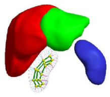
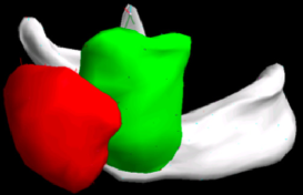
(a)                                         (b)

Figure 1. Examples of 3-dimensional medical images (obtained by MIDAG at UNC Chapel Hill) of a collection of physiological objects which can be modeled by a multi-region configuration. a) Prostate, bladder and rectum in pelvic region and b) mandible, masseter muscle, and parotid gland in throat region.

The goal of this paper is to introduce for such configurations “medial and skeletal linking structures”, which allow us to simultaneously capture shape properties of the individual objects and their “positional geometry”.

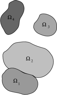
Figure 2. Multi-region configuration in ${\mathbb{R}}^{2}$.

Such structures build on earlier work in which the first author developed the notion of a “skeletal structure”for a single compact region $\Omega$ with smooth boundary $\mathcal{B}$ [D1]. It consists of a pair $(M,U)$, where the “skeletal set”$M$ is a Whitney stratified set in the region and $U$ is a multivalued “radial vector field”defined on $M$. Skeletal structures generalize the notion of the Blum medial axis of a region with smooth boundary [BN] (also called the “central set”, see [Y]), which is the locus of centers of spheres in $\Omega$ tangent to $\mathcal{B}$ at two or more points (or having a single degenerate tangency). The Blum medial axis is a special type of skeletal structure (with $U$ consisting of the vectors from points of $M$ to the points of tangency).

The Blum medial axis $M$ captures the shape of a region. It has several alternate descriptions as the shock set of the “grassfire/eikonal flow”from the boundary as in Kimia-Tannenbaum-Zucker [KTZ] and as the Maxwell set of the family of “distance to the boundary functions”, see Mather [M2]. These multiple descriptions have allowed for the classification of the local structure of $M$ for regions with generic boundaries $\mathcal{B}$ [Y], [M2], [Gb], [GK]. In addition, these have led to several different methods for computing the medial axis using properties of the grassfire/eikonal flow [BSTZ], [DDS] and Voronoi methods (see [PS] for a survey of these methods) and a recent method using B-spline representations to directly evolve the medial axis [MCD].

The skeletal structure relaxes several of the conditions in the Blum case, and allows more flexibility in applying skeletal structures to model objects including: using skeletal structures as deformable templates for modeling objects [P], overcoming the lack of $C^{1}$-stability of the Blum medial axis, allowing alternate models based on a region being swept out by a family of hyperplanes, [D7] and the related [GK2], and providing discrete models to which statistical analysis can be applied [P2], [PJG]. This has enhanced their usefulness for modeling and computer imaging questions for medicine and biology (see e.g. [PS] for a survey of results).

Furthermore, the structure enables both the local, relative, and global geometric properties of the region and its boundary to be computed from the “medial geometry”of the radial vector field on the skeletal structure [D2], [D3], [D4]. This includes conditions ensuring the nonsingularity of a “radial flow”from the skeletal set to the boundary. This allows the region to be fibered with the level sets of the flow and implies the smoothness of the boundary [D1, Thm 2.5]. As the Blum medial axis is a special type of skeletal structure these results also apply to it, and to the related “symmetry-set”[BGG].

In this paper, we introduce the “medial and skeletal linking structures”  which build upon individual skeletal structures of the regions in a minimal way, but still enable us to analyze the positional geometry of the configuration along with the shapes of the individual regions. The added structure consists of a multivalued “linking function”$\ell_{i}$ defined on the skeletal set $M_{i}$ for each region $\Omega_{i}$ and a refinement of the Whitney stratification of $M_{i}$ on which it is stratawise smooth. The linking functions $\ell_{i}$ together with the radial vector fields $U_{i}$ yield multivalued “linking vector fields”$L_{i}$, which satisfy certain linking conditions. Even though the structures are defined on the skeletal sets within the regions, the linking vector fields allow us to capture geometric properties of the external region as well. In addition, we identify the regions which are unlinked and classify their local generic structure by introducing the spherical axis which is the analog of the Blum medial axis but for the family of height functions on the region boundaries.

The paper is divided into four parts. In Part I, we define and give the basic properties of medial/skeletal linking structures and state two theorems assuring the existence of a skeletal linking structure for generic configurations. First, for a general generic multi-region configuration with singular shared boundaries, we establish the existence of a generic “full Blum linking structure”for the configuration (Theorem 4.18). In the special case where all of the regions are disjoint with smooth generic boundaries, this yields a “Blum medial linking structure”(Theorem 4.17). This special case for disjoint regions was obtained in the thesis of the second author [Ga]. Then, in the case of a generic configuration with singular boundaries, the Blum structure now contains the singular points of the boundaries in its closure and we give an “edge-corner normal form”near such singular points. This requires providing an addendum (Theorem 4.5) to the result of Mather [M2] for a single region, where we now allow a singular boundary. In Section 5 we explain how to modify the resulting Blum structure to obtain a skeletal linking structure.

In Part II, we use the linking structure to determine properties of the “positional geometry”of the configuration. We introduce and compute several invariants of the positional geometry, and deduce properties of these invariants. These use the linking flow (which extends the radial flow into the external region) and allows the determination of the linking neighborhoods between regions. The nonsingularity of the linking flow will follow from linking curvature conditions on the linking functions, having a form analogous to those given in [D1, Thm 2.5] for the radial flow.

This allows us to introduce invariants which include measures of relative closeness and positional significance of the individual regions for the configuration. These are given in terms of volumetric measurements on the regions themselves and on associated regions defined by the linking flow. The measure of significance allows us to identify the central regions as well as outliers from among the regions. We prove that using the linking structure, we can compute these volumetric invariants (which involve regions outside the configuration) as “skeletal linking integrals”on the internal skeletal sets. These invariants are then used to construct a “tiered linking graph”. When given thresholds of closeness and significance are applied to this graph, they yield subgraph(s) identifying subconfigurations and provide a hierarchical ordering of the regions. The skeletal linking structure also allows for the comparison and statistical analysis of collections of objects in ${\mathbb{R}}^{n+1}$, extending the analyses given in earlier work for single regions.

In Parts III and IV, we prove the existence and derive the generic properties of the (full) Blum linking structure. The properties of the Blum structure result from generic properties of several associated “multi-functions”which include “multi-distance functions”and “height-distance functions”. Because these latter functions are examples of divergent diagrams of functions, the usual theorems of singularity theory do not apply (see e.g. [DF]). Nonetheless, in Part III we prove a multi-transversality theorem (Theorem 13.2) which applies to the multi-functions relative to a “partial multijet space”. This yields the generic properties for the Blum linking structures for an open dense set of the space of embeddings of configurations of each given type. This transversality theorem extends earlier transversality theorems for families of functions due to Looijenga [L] and Wall [Wa] and is based on a “hybrid transversality theorem”(Theorem 16.5) using results from [D5].

In Part IV we construct the families of perturbations needed for applying the transversality theorems. We then carry out the necessary derivative computations needed to prove the applicability of the transversality theorems to the space of embeddings of a configuration. This allows us to deduce for an open dense set of mappings the existence of the Blum linking structures with their generic properties.

The authors would like to thank Stephen Pizer for sharing with us his early work with his coworkers on medical imaging involving multiple objects in medical images. This led us to seek a completely mathematical approach to these problems. We also are very grateful to the several referees for their careful reading and multiple suggestions for improving the exposition in the paper, and to the editor Alejandro Adem for his considerable help in moving the process forward. Hopefully the final version reflects all of this.

Overview of the Genericity and Transversality Results

To establish the results of this paper for the generic properties of the geometric structures, we will carry out extensions of earlier work of Mather [M2], Looijenga [L], and Wall [Wa]. We indicate exactly the form that these extensions will ultimately take.

First, in the Blum case, rather than consider the disjoint Blum medial axes for different regions, we consider the “generic linking properties”  for the distinct regions. This forces us to consider the interplay between the stratifications on the boundaries that arise from the individual Blum medial axes and the stratification resulting from the family of height functions. These interactions result from having two distance functions or a distance function and a height function at the same point. This problem already arises in the case of distinct regions with smooth boundaries as the linking occurs via the complementary region. To handle this situation we introduce transversality theorems for multi-functions, which will yield the generic interplay between the stratifications. These “hybrid transversality theorems”  allow us to prove transversality for the multijets of such multi-functions relative to partial jet spaces, which are subbundles of jet bundles. We apply these theorems in the context of continuous mappings from Baire spaces of embeddings of configurations to the spaces of parametrized families of functions. These theorems extend earlier relative and absolute transversality theorems in [D5].

Second, Mather’s results for the Blum medial axis concentrated on the local structure of the Blum medial axis by using a multi-germ versality theorem. This by itself does not imply anything about the corresponding properties of points on the boundaries corresponding to the medial axis points. Several partial results were obtained by Porteous [Po] and Bruce-Giblin-Tari [BGT] from the point of view of the geometry of the boundary as a surface. We address this by establishing a general result for the resulting stratifications of the boundary by the “generic linking type”  of the points. We also apply the transversality theorem of Wall for the family of height functions and our extension for “height-distance”  functions to give the generic properties of the “spherical axis”, the resulting properties of the stratification of the unlinked region, and its relation with the Blum stratifications on the boundaries.

Third, one of the principal extensions is to collections of regions allowing boundaries and corners where the regions may share portions of their boundaries allowing specific generic local forms. The methods we develop allow us to include these nonsmooth features in our analysis. For the global theory we prove special versions of the transversality theorem to overcome the problem on stratified sets in several ways. This depends upon replacing the Seeley extension theorem [Se] used by Mather with a more general extension theorem due to Bierstone [Bi]. This then extends traditional transversality theorems so they can apply to this situation. One consequence is to provide an addendum to Mather’s theorem on the local generic form of the Blum medial axis for a region with generic smooth boundary to the case where the region has a generic boundary with corners.

Fourth, genericity proved from the multi-transversality theorems only yields the results for a residual set of mappings of configurations. By contrast, Mather [M2] asserts that the generic set of embeddings for the Blum medial structure form an open set, although he does not prove it in his paper. We give a treatment in our general case to prove that the set of smooth embeddings of configurations which exhibit the generic linking properties forms an open set in the space of smooth embeddings (and hence smooth mappings). We do so by relating the versality of the distance and height functions with the infinitesimal stability of associated mappings, and then applying Mather’s general theorem “infinitesimal stability implies stability”[M5].

CONTENTS

• Medial/Skeletal Linking Structures

• Multi-Region Configurations in ${\mathbb{R}}^{n+1}$

  Local Models for Regions at Singular Points on Boundary

  The Space of Equivalent Configurations via Mappings of a Model

  Configurations allowing Containment of Regions

• Skeletal Linking Structures for Multi-Region Configurations in ${\mathbb{R}}^{n+1}$

  Skeletal Linking Structures for Multi-Region Configurations

  Linking between Regions and between Skeletal Sets

• Blum Medial Linking Structure for a Generic Multi-Region Configuration

  Blum Medial Axis for a Single Region with Smooth Generic

  Boundary

  Addendum to Generic Blum Structure for a Region with

  Boundaries and Corners

  Blum Medial Linking Structure

  Generic Linking Properties

  Existence of Blum Medial Linking Structure

  Addendum: Classification of Linking Types for Blum Medial

  Linking Structures in ${\mathbb{R}}^{3}$

• Retracting the Full Blum Medial Structure to a Skeletal Linking Structure

• Positional Geometry of Linking Structures

• Questions Involving Positional Geometry of a Multi-region Configuration

  Introduction

• Shape Operators and Radial Flow for a Skeletal Structure

  The Radial Flow

  Radial and Edge Shape Operators

  Curvature Conditions and Nonsingularity of the Radial Flow

  Evolution of the Shape Operators under the Radial Flow

• Linking Flow and Curvature Conditions

  Nonsingularity of the Linking Flow

  Special Möbius Transformations of Matrices and Operators

  Evolution of the Shape Operators under the Linking Flow

• Properties of Regions Defined Using the Linking Flow

  Medial/Skeletal Linking Structures in the Unbounded Case

  Medial/Skeletal Linking Structures for the Bounded Case

• Global Geometry via Medial and Skeletal Linking Integrals

  Defining Medial and Skeletal Linking Integrals

  Computing Boundary Integrals via Medial Linking Integrals

  Computing Integrals as Skeletal Integrals via the Linking Flow

  Skeletal Linking Integral Formulas for Global Invariants

• Positional Geometric Properties of Multi-Region Configurations

  Neighboring Regions and Measures of Closeness

  Measuring Significance of Objects Via Linking Structures

  Properties of Invariants for Closeness and Significance

  Tiered Linking Graph

  Higher Order Positional Geometric Relations via Indirect Linking

• Generic Properties of Linking Structures via Transversality Theorems

• Multi-Distance and Height-Distance Functions and Partial Multijet Spaces

  Multi-Distance and Height-Distance Functions

  Partial Jet Spaces for Multi-Distance and Height-Distance

  Functions

• Generic Blum Linking Properties via Transversality Theorems

  Transversality Theorem for Multi-Distance and Height-Distance

  Functions

  Strata for Generic Properties of Blum Linking Structure

• Generic Properties of Blum Linking Structures

  Properties of Transversality and Whitney Stratified Sets

  Consequences of Transversality for Multi-Distance Functions

  Consequences of Transversality for Height-Distance Functions

  Proof of Theorem 4.17 for a Residual Set of Embeddings

• Concluding Generic Properties of Blum Linking Structures

  Blum Medial Structure near Corner Points

  Openness of the Genericity Conditions

• Proofs and Calculations for the Transversality Theorems

• Reductions of the Proofs of the Transversality Theorems

  Hybrid Transversality Theorem

  Multi-Jet Properties Implying Stratification Properties

  on the Boundaries

• Families of Perturbations and their Infinitesimal Properties

  Construction of the Families of Perturbations

  Computation of Derivatives for Families of Perturbations

  Jet Properties of Parameter Deformations

• Completing the Proofs of the Transversality Theorems

  Perturbation Transversality Conditions via Fiber Jet Extension Maps

  Computing Derivatives of the Multi-functions at Critical Points

  Concluding the Proofs

• Appendix: List of Frequently Used Notation

2. Multi-Region Configurations in ${\mathbb{R}}^{n+1}$

Local Models for Regions at Singular Points on Boundary

We begin by defining what exactly we mean by a “multi-region configuration”. First, we consider compact connected $n+1$- dimensional regions $\Omega\subset{\mathbb{R}}^{n+1}$ which are smooth manifolds with boundaries and corners, with boundaries denoted by $\mathcal{B}$. We recall that $\Omega$ is a manifold with boundaries and corners if each point $x\in\mathcal{B}$ has a neighborhood $U\subset\Omega$ diffeomorphic, with $x\mapsto 0$, to an open subset of $C_{k}={\mathbb{R}}^{k}_{+}\times{\mathbb{R}}^{n+1-k}$, for some $0\leq k\leq n$. We refer to such $x$ as a $k$-edge-corner point. Here ${\mathbb{R}}^{k}_{+}=\{(x_{1},\dots,x_{k})\in{\mathbb{R}}:x_{i}\geq 0\}$. Then $\mathcal{B}$ is stratified by the strata consisting of $k$-edge-corner points $x\in\mathcal{B}$. Those strata of dimension $n$ will be referred to as the open (or regular) strata of the boundary.

Second, we require that the regions satisfy the boundary intersection condition: if two such regions intersect, they do so only on their boundaries; and their common intersection is a union of strata (defined above). Third, the regions satisfy the boundary edge condition: if a point $x$ is contained in more than one region then the union of the boundaries of the regions containing $x$ is locally diffeomorphic in a neighborhood of $x$ to one of the following regions $P_{k}$ or $Q_{k}$ in ${\mathbb{R}}^{n+1}$ for $k=1,\dots n+1$.

For $y=(y_{1},\dots,y_{k+1})\in{\mathbb{R}}^{k+1}$, we let $g_{k+1}(y)=\sum_{i=1}^{k+1}y_{i}$. Then, we may identify ${\mathbb{R}}^{n+1}$ with $L_{k}\times{\mathbb{R}}^{n+1-k}$ where $L_{k}=\{y\in{\mathbb{R}}^{k+1}:g_{k+1}(y)=0\}$. We then define

• $P_{k}=Y_{k}\times{\mathbb{R}}^{n+1-k}$, where

  $$Y_{k}=\{y\in L_{k}:\text{for some }i\neq j,\,y_{i}=y_{j}\leq y_{\ell}\text{ for }\ell\neq i,j\}$$

  and for $1\leq k\leq n$,

• $Q_{k}=Z_{n+1}\cup(H_{n+1}\cap P_{k})$,

where for $(y,x)\in L_{k}\times{\mathbb{R}}^{n+1-k}$ with $x=(x_{k+1},\dots,x_{n+1})\in{\mathbb{R}}^{n-k+1}$, $Z_{n+1}$ is the hyperplane defined by $x_{n+1}=0$, and $H_{n+1}$ is the half-space defined by $x_{n+1}\geq 0$.

The local forms for ${\mathbb{R}}^{3}$ consist of a smooth surface together with those shown in Figure 3.

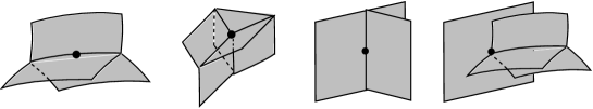
(a)                    (b)               (c)                    (d)

Figure 3. Generic local forms for intersecting regions in ${\mathbb{R}}^{3}$: a) $P_{2}$; b) $P_{3}$; c) $Q_{1}$; and d) $Q_{2}$.

We note that $P_{1}$ denotes a smooth boundary region of each of two regions, so a point of the common boundary region will be in the closure of the open strata unless it is a point where more than two regions (including the exterior) meet. For $k>1$, a $P_{k}$-point of a region $\Omega_{i}$ will be a singular point of the boundary, and hence lies in the singular set of $\mathcal{B}_{i}$.

By contrast, there are two possibilities for $Q_{k}$-points. First, a region may have for its boundary the hypersurface $Z_{n+1}$ in the local model at a $Q_{k}$-point. We refer to the point as a smooth $Q_{k}$-point. Second, the boundary in the local model at a $Q_{k}$-point may be formed from both part of $Z_{n+1}$ and a face from $P_{k}$ in the local model. The $Q_{k}$-point will be a singular point of its boundary, and we refer to it as a singular $Q_{k}$-point. For a region $\Omega_{i}$, the set of smooth $Q_{k}$-points for all $k$ defines a compact Whitney stratified set $\Sigma_{Q\,i}$. This locally consists of the intersection of $Z_{n+1}$ with the other faces. It is contained in the set of smooth points of the boundary $\mathcal{B}_{i}$. We let $\Sigma_{Q}=\cup_{i}\Sigma_{Q\,i}$.

Remark 2.1.

For the local configurations in a) and b) in Figure 3, one of the complementary regions may denote the external complement of the union of regions. For c) and d), only one of the regions to the right of the plane may be a complementary external region. Physically such local configurations of type a) or b) arise when regions with flexible boundaries have physical contact. This includes the singularities in soap bubbles. For c) and d), the region to the left of the plane would represent a rigid region with which one or more flexible regions have contact.

Definition 2.2.

A multi-region configuration consists of a collection of compact $(n+1)$-dimensional regions $\Omega_{i}\subset{\mathbb{R}}^{n+1}$, $i=1,\dots,m$, which have smooth boundaries with corners, with boundaries denoted by $\mathcal{B}_{i}$, and satisfying the boundary intersection condition and the boundary edge condition.

For a given configuration of regions $\boldsymbol{\Omega}=\{\Omega_{i}\}_{i=1}^{m}$, the union $\cup_{i=1}^{m}\Omega_{i}$ has a Whitney stratification consisting of the interiors of the $\Omega_{i}$ together with the strata of the boundaries of the $\Omega_{i}$ formed from the $k$-edge-corner points for each given $k$, and their complement consisting of smooth points of each boundary (for detailed treatments of Whitney stratifications and their properties see e.g. [Wh], [M1], [M3], or [GLDW]). Also, we let $\Omega_{0}$ denote the closure of the complement ${\mathbb{R}}^{n+1}\backslash\cup_{i=1}^{m}\Omega_{i}$.

The Space of Equivalent Configurations via Mappings of a Model

In order to consider generic configurations, we describe how we will deform such a configuration of regions preserving the form of the intersections via mappings of the configuration. Let $\boldsymbol{\Delta}$ be a configuration of multi-regions $\{\Delta_{i}\}$ (in ${\mathbb{R}}^{n+1}$) satisfying Definition 2.2.

Definition 2.3.

A multi-region configuration $\boldsymbol{\Omega}$ based on model configuration $\boldsymbol{\Delta}$ is given by a smooth embedding $\Phi:\boldsymbol{\Delta}\to{\mathbb{R}}^{n+1}$ which restricts to diffeomorphisms $\Delta_{i}\simeq\Omega_{i}$ for each $i$. Multi-region configurations with model configuration $\boldsymbol{\Delta}$ will be said to be configurations of the same type as $\boldsymbol{\Omega}$.

The space of configurations of type $\boldsymbol{\Delta}$ is given by the space of embeddings ${\rm Emb}\,(\boldsymbol{\Delta},{\mathbb{R}}^{n+1})$ with the $C^{\infty}$-topology.

For such a configuration, we let the boundary of $\Delta_{i}$ be denoted by $X_{i}$ and then $\mathcal{B}_{i}=\Phi(X_{i})$ is the boundary of $\Omega_{i}$. Even though the configuration varies with $\Phi$ we still use the notation $\boldsymbol{\Omega}$ for the resulting (varying) image configuration (with a specific $\Phi$ understood). We have the stratification of $\boldsymbol{\Delta}$ as described above and by applying $\Phi$ we obtain a corresponding stratification of $\boldsymbol{\Omega}$.

We note that the union of the regions can be viewed as a manifold with boundaries and corners except edges and corners are inward pointing. Nonetheless, we shall see that the basic properties that are used for mappings on manifolds with boundaries and corners will still be valid.

Figure 4. A multi-region configuration in ${\mathbb{R}}^{2}$. The stratification consists of the interiors of the regions, the open boundary curves, excluding branch points which are either of type $P_{2}$ or $Q_{1}$.

Definition 2.4.

The regions $\Delta_{i}$ and $\Delta_{j}$ are adjoining regions if $X_{i}\cap X_{j}\neq\emptyset$. If $X_{i}\backslash\cup_{j\neq i}X_{j}\neq\emptyset$, we say $\Delta_{i}$ adjoins the complement. These then have the corresponding meanings for the image regions $\Omega_{i}$, $\Omega_{j}$ and $\Omega_{0}$.

Remark 2.5.

In the special case of a configuration consisting of disjoint regions with smooth boundaries, each region is thus only adjoined to the complement. Then, we shall see that the geometric relations between the regions will be captured only via linking behavior in the external region.

As all of the $\Delta_{i}$ are compact, $\Phi(\boldsymbol{\Delta})$ is compact and hence bounded. However, we introduce a stronger notion of being bounded. If we are given an ambient region $\tilde{\Omega}$ so that $\Omega_{i}\subset{\rm int}\,(\tilde{\Omega})$ for each $i$, then we say that $\boldsymbol{\Omega}$ is a configuration bounded by $\tilde{\Omega}$. Then we may either consider bounded configurations given by an embedding $\tilde{\Phi}:\tilde{\Delta}\to{\mathbb{R}}^{n+1}$, with $\tilde{\Phi}(\tilde{\Delta})$ denoting $\tilde{\Omega}$, and $\Phi=\tilde{\Phi}|\boldsymbol{\Delta}$; or fix $\tilde{\Omega}$ and consider embeddings $\Phi:\boldsymbol{\Delta}\to{\rm int}\,(\tilde{\Omega})$. Such a $\tilde{\Omega}$ might be a bounding box or disk or an intrinsic region containing the configuration, for examples see §9.

Configurations allowing Containment of Regions

In our definition of a multi-region configuration, we have explicitly excluded one region being contained in another. However, given a configuration which allows this, we can easily identify such a configuration with the type we have already given. To do so, we require that the boundaries of two regions still intersect in a union of strata which form the closure of strata of dimension $n$. Then, if one region is contained in another $\Omega_{i}\subset\Omega_{j}$, then we may represent $\Omega_{j}$ as a union of two regions $\Omega_{i}$ and the closure of $\Omega_{j}\backslash({\rm int}\,(\Omega_{i})\cup(\mathcal{B}_{i}\cap\mathcal{B}_{j}))$, which we refer to as the region complement to $\Omega_{i}$ in $\Omega_{j}$. By repeating this process a number of times we arrive at a representation of the configuration as a multi-region configuration in the sense of Definition 2.2. See Figure 5.

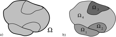
Figure 5. a) is a configuration of regions contained in a region $\Omega$. It is equivalent to a multi-region configuration b) which is without inclusion. Note that in this representation, the boundary of contained regions will meet in a transverse fashion, any boundary region of the containing region.

3. Skeletal Linking Structures for Multi-Region Configurations in ${\mathbb{R}}^{n+1}$

The skeletal linking structures for multi-region configurations will build upon the skeletal structures for individual regions. We begin by recalling their basic definitions and simplest properties.

Skeletal Structures for Single Regions

We begin by recalling [D1] that a “skeletal structure”$(M,U)$ in ${\mathbb{R}}^{n+1}$, [D1, Def. 1.13], consists of: a Whitney stratified set $M$ and a multivalued “radial vector field”  $U$ on $M$. We will not give every condition in detail, but instead point out the key features and just mention certain technical conditions that are needed so the structure has the correct global properties.

$M$ satisfies the conditions for being a “skeletal set”  [D1, Def. 1.2], which we briefly recall. The skeletal set $M$ consists of smooth strata of dimension $n$, denoted by $M_{reg}$, and the set of singular strata $M_{sing}$, with $\partial M$ denoting the singular strata where $M$ is locally a manifold with boundary (for which we must use special “boundary coordinates”, see [D1, Def. 1.3]). It satisfies the following properties.

• For each point $x_{0}\in M_{sing}$, and each connected component $M_{\alpha}$ of $M_{reg}$ in a sufficiently small neighborhood of $x_{0}$, there is a unique limiting tangent space $\lim T_{x_{i}}M_{\alpha}$ for any sequence $\{x_{i}\}\subset M_{\alpha}$ converging to $x_{0}$.

• Locally in a neighborhood of a singular point $x_{0}$, $M$ may be expressed as a union of (smooth) $n$–manifolds with boundaries and corners $M_{\alpha_{j}}$, where two such intersect only on boundary facets (faces, edges etc.). We will refer to this as a “paved neighborhood”  of $x_{0}$ (see Figure 6).

• If $x_{0}\in\overline{\partial M}$ then those $M_{\alpha_{j}}$ in (2) meeting $\partial M$ meet it in an $n-1$ dimensional facet.

Condition ii) is a simplified form of a local triangulation of a stratified set, see [Go], [V].

Second, the multivalued vector field $U$ has the following properties.

• For each smooth point $x_{0}\in M_{reg}$, there are two values of $U$ which point toward opposite sides of $T_{x_{0}}M$. Moreover, on a neighborhood of a point of $M_{reg}$, the values of $U$ corresponding to one side form a smooth vector field.

• For a singular point $x_{0}\notin\partial M$, with $M_{\alpha_{j}}$ a connected component containing $x_{0}$ in its closure, both smooth values of $U$ on $M_{\alpha}$ extend smoothly to values $U(x_{0})$ on the stratum of $x_{0}$. If $M_{\alpha_{j}}$ does not intersect $\partial M$ in a neighborhood of $x_{0}$, then $U(x_{0})\notin T_{x_{0}}M_{\alpha_{j}}$. In addition, for each local connected component $C_{i}$ of $B_{\varepsilon}(x_{0})\cap({\mathbb{R}}^{n+1}\backslash M)$ in a small ball $B_{\varepsilon}(x_{0})$, there is a unique value of $U$ pointing into $C_{i}$ and the values at points in a neighborhood $B_{\varepsilon}(x_{0})\cap M$ of $x_{0}$ which point into $C_{i}$ define a continuous vector field which is smooth on each stratum of $M$ (see a) in Figure 6 or Figure 9).

• At points $x_{0}\in\partial M$, there is a unique value for $U$ which is tangent to the stratum of $M_{reg}$ containing $x_{0}$ in the closure and points away from $M$.

When we refer to a smooth value of $U$ at $x_{0}$ we mean either a smoothly varying choice of $U$ on one side of $M$ if $x_{0}\in M_{reg}$ or one on $M_{\alpha_{j}}$ extending smoothly to $x_{0}$ if $x_{0}\in M_{sing}$. This allows various mathematical constructions on the smooth strata to be extended to the singular strata $M_{sing}$, see [D1, §2].

Using the multivalued radial vector field $U$, we can define a stratified set (with smooth strata) $\tilde{M}$, called the “double of $M$”. Points of $\tilde{M}$ consist of all pairs $\tilde{x}=(U,x)$ where $U$ is a value of the radial vector field at $x$, and neighborhood of points $\tilde{x}$ are defined in $\tilde{M}$ using continuous extensions of $U$ near $x$. For example, the neighborhood in a) of Figure 6 gives the neighborhoods in $\tilde{M}$ corresponding to b) and c). There is also defined a finite-to-one stratified mapping $\pi:\tilde{M}\to M$ defined by $\pi(U,x)=x$, see [D1, §3].

On $\tilde{M}$ is defined a “normal line bundle”$N$, such that over $\tilde{x}=(U,x)$, $N_{\tilde{x}}=\{a\cdot U:a\in{\mathbb{R}}\}$. It is a trivial line bundle, with a “half-line bundle”  $N_{+}=\{c\cdot U:c\geq 0\}$. We also define “one-sided neighborhoods”of the zero section $N_{a}=\{c\cdot U:0\leq c\leq a\}$.

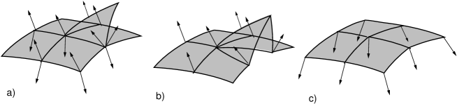
Figure 6. a) illustrates a “paved neighborhood”of a point in $M$ showing the paving by manifolds with boundaries and corners and the multivalued vector fields pointing to the local complementary components. b) and c) illustrate the two corresponding paved neighborhoods in $\tilde{M}$.

Then, using $\tilde{M}$, we can define the “radial flow”. In a neighborhood $W$ of a point $x_{0}\in M$ with a smooth single-valued choice for $U$, we define a local representation of the radial flow by $\psi_{t}(x)=x+t\cdot U(x)$. It yields a global radial flow as a mapping $\Psi:N_{+}\to{\mathbb{R}}^{n+1}$. Lastly, there are two technical conditions for a skeletal structure, the “local initial conditions”[D1, Def. 1.7] which ensure that the radial flow for small time remains one-to one (and stratawise nonsingular).

We also recall from [D1] that beginning with a skeletal structure $(M,U)$ in ${\mathbb{R}}^{n+1}$, we associate a “region”$\Omega=\Psi(N_{1})$ and its “boundary”$\mathcal{B}=\{x+U(x):x\in M\,\mbox{ all values of }U\}$. Then, provided certain curvature and compatibility conditions are satisfied, which we will recall in §7, it follows by [D1, Thm 2.5] that the radial flow defines a stratawise smooth diffeomorphism between $N_{1}\backslash\tilde{M}$ and $\Omega\backslash M$, with the boundary. From the radial flow we define the radial map $\psi_{1}(x)=x+U(x)$ from $\tilde{M}$ to $\mathcal{B}$. We may then relate the boundary and skeletal set via the radial flow and the radial map.

A standard example we consider will be the Blum medial axis $M$ of a region $\Omega$ with generic smooth boundary $\mathcal{B}$ and its associated (multivalued) radial vector field $U$. Then, the associated boundary $\mathcal{B}$ we consider here will be the initial boundary of the object.

Skeletal Linking Structures for Multi-Region Configurations

We are ready to introduce skeletal linking structures for multi-region configurations. These structures will accomplish multiple goals. The most significant are the following.

• Extend the skeletal structures for the individual regions in a minimal way to obtain a unified structure which also incorporates the positional information of the objects.

• For generic configurations of disjoint regions with smooth boundaries, provide a Blum medial linking structure which incorporates the Blum medial axes of the individual objects.

• For general multi-region configurations with common boundaries, provide for a modification of the resulting Blum structure to give a skeletal linking structure.

• Handle both unbounded and bounded multi-region configurations.

Later we shall also see that the skeletal linking structure has a second important function allowing us to answer various questions involving the “positional geometry”of the regions in the configuration.

We begin by giving versions of the definition for both the bounded and unbounded cases.

Definition 3.1.

A skeletal linking structure for a multi-region configuration $\{\Omega_{i}\}$ in ${\mathbb{R}}^{n+1}$ consists of a triple $(M_{i},U_{i},\ell_{i})$ for each region $\Omega_{i}$ with the following two sets of properties.

• $(M_{i},U_{i})$ is a skeletal structure for $\Omega_{i}$ for each $i$ with $U_{i}=r_{i}\cdot\mathbf{u}_{i}$ for $\mathbf{u}_{i}$ a (multivalued) unit vector field and $r_{i}$ the multivalued radial function on $M_{i}$.

• $\ell_{i}$ is a (multivalued) linking function defined on $M_{i}$ (excluding the strata $M_{i\,\infty}$, see L4 below), with one value for each value of $U_{i}$, for which the corresponding values satisfy $\ell_{i}\geq r_{i}$, and it yields a (multivalued) linking vector field $L_{i}=\ell_{i}\cdot\mathbf{u}_{i}$ .

• The canonical stratification of $\tilde{M}_{i}$ has a stratified refinement $\mathcal{S}_{i}$, which we refer to as the labeled refinement.

By $\mathcal{S}_{i}$ being a “labeled refinement”of the stratification $\tilde{M}_{i}$ we mean it is a refinement in the usual sense of stratifications in that each stratum of $\tilde{M}_{i}$ is a union of strata of $\mathcal{S}_{i}$; and they are labeled by the linking types which occur on the strata.

In addition, they satisfy the following four linking conditions.

Conditions for a skeletal linking structure

• $\ell_{i}$ and $L_{i}$ are continuous where defined on $M_{i}$ and are smooth on strata of $\mathcal{S}_{i}$.

• The “linking flow”(see (3.1) below) obtained by extending the radial flow is nonsingular and for the strata $S_{i\,j}$ of $\mathcal{S}_{i}$, the images of the linking flow are disjoint and each $W_{i\,j}=\{x+L_{i}(x):x\in S_{ij}\}$ is smooth.

• The strata $\{W_{i\,j}\}$ from the distinct regions either agree or are disjoint and together they form a stratified set $M_{0}$, which we shall refer to as the (external) linking axis.

• There are strata $M_{i\,\infty}\subset\tilde{M}_{i}$ on which there is no linking so the linking function $\ell_{i}$ is undefined. On the union of these strata $M_{\infty}=\cup_{i}M_{i\,\infty}$, the global radial flow restricted to $N_{+}|M_{\infty}$ is a diffeomorphism with image the complement of the image of the linking flow. In the bounded case, with $\tilde{\Omega}$ the enclosing region of the configuration, it is required that the boundary of $\tilde{\Omega}$ is transverse to the stratification of $M_{0}$ and where the linking vector field extends beyond $\tilde{\Omega}$, it is truncated at the boundary of $\tilde{\Omega}$ (this includes $M_{\infty}$).

We denote the region on the boundary corresponding to $M_{\infty}$ by $\mathcal{B}_{\infty}$ and that corresponding to $M_{i\,\infty}$ by $\mathcal{B}_{i\,\infty}$.

Remark 3.2.

By property L4), $\mathcal{B}_{i\,\infty}$ does not exhibit any linking with any other region. We will view it as either the unlinked region or alternately as being linked to $\infty$, where we may view the linking function as being $\infty$ on $M_{i\,\infty}$. In the bounded case with $\tilde{\Omega}$ the enclosing region of the configuration, we modify the linking vector field so it is truncated at the boundary of $\tilde{\Omega}$. We can also introduce a “linking vector field on $M_{\infty}$”  by extending the radial vector field until it meets the boundary of $\tilde{\Omega}$. Then, in the bounded case, we let $M_{b}$ denote the set of points in $\tilde{M}$ whose linking vector fields end at the boundary of $\tilde{\Omega}$. Then, $M_{\infty}\subseteq M_{b}\subset\tilde{M}$, and in the generic bounded case, $M_{b}$ has a natural stratification, and it provides the linking to the boundary of $\tilde{\Omega}$.

For this definition, we must define the “linking flow”  which is an extension of the radial flow. We define the linking flow from $M_{i}$ by

(3.1) $$\lambda_{i}(x,t)\,\, =\,\,x\,+\,\chi_{i}(x,t)\mathbf{u}_{i}(x)\qquad\text{where}$$

(3.4) $$\chi_{i}(x,t) =\left\{\begin{array}[]{lr}2tr_{i}(x)&\displaystyle 0\leq t\leq\frac{1}{2}\\ 2(1-t)r_{i}(x)+(2t-1)\ell_{i}(x)&\displaystyle\frac{1}{2}\leq t\leq 1\end{array}\right.\,.$$

As with the radial flow it is actually defined from $\tilde{M}_{i}$ (or $\tilde{M}_{i}\backslash M_{\infty}$). The combined linking flows $\lambda_{i}$ from all of the $M_{i}$ will be jointly referred to as the linking flow $\lambda$. For fixed $t$ we will frequently denote $\lambda(\cdot,t)$ by $\lambda_{t}$.

Convention: Because we will often view the collection of objects for the linking structure as together forming a single object, we will adopt notation for the entire collection. This includes $M$ for the union of the $M_{i}$ for $i>0$, and similarly for $\tilde{M}$. On $M$ (or $\tilde{M}$) we have the radial vector field $U$ and radial function $r$ formed from the individual $U_{i}$ and $r_{i}$, the linking function $\ell$ and linking vector field $L$ formed from the individual $\ell_{i}$ and $L_{i}$; as well as the linking flow $\lambda$ and $M_{\infty}$ already defined.

We see that for $0\leq t\leq\frac{1}{2}$ the flow is the radial flow at twice its speed; hence, the level sets of the linking flow, $\mathcal{B}_{i\,t}$, for time $0\leq t\leq\frac{1}{2}$ will be those of the radial flow. For $\frac{1}{2}\leq t\leq 1$ the linking flow is from the boundary $\mathcal{B}_{i}$ to the linking strata of the external medial linking axis.

By the linking flow being nonsingular we mean it is a piecewise smooth homeomorphism, which for each stratum $S_{i\,j}\subset\tilde{M}_{i}$, is smooth and nonsingular on $S_{i\,j}\times\left[0,\frac{1}{2}\right]$. Also, either: $S_{i\,j}\times\left[\frac{1}{2},1\right]$ is smooth and nonsingular if $S_{i\,j}$ is a stratum associated to strata in $\mathcal{B}_{i\,0}$; or $S_{i\,j}$ is not associated to strata in $\mathcal{B}_{i\,0}$, $\ell_{i}=r_{i}$ on $S_{i\,j}$, and so the linking flow on $S_{i\,j}\times\left[\frac{1}{2},1\right]$ is constant as a function of $t$. That the linking flow is nonsingular will follow from the analogue of the conditions given in [D1, §3] for the nonsingularity of the radial flow. These will be given later, when we use the linking flow to establish geometric properties of the configuration.

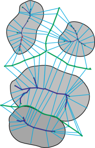
Figure 7. Skeletal linking structure for multi-region configuration in ${\mathbb{R}}^{2}$. Note that the linking axis includes the shared boundary curves of adjoined regions.

In Figure 7 we illustrate (a portion of) the skeletal linking structure for a configuration of four regions. Shown are the linking vector fields meeting on the (external) linking axis. The linking flow moves along the lines from the medial axes to meet at the linking axis.

Linking between Regions and between Skeletal Sets

A skeletal linking structure allows us to introduce the notion of linking of points in different (or the same) regions and of regions themselves being linked. We say that two points $x\in\tilde{M}_{i}$ and $x^{\prime}\in\tilde{M}_{j}$ are linked if the linking flows satisfy $\lambda_{i}(x,1)=\lambda_{j}(x^{\prime},1)$. This is equivalent to saying that for the values of the linking vector fields $L_{i}(x)$ and $L_{j}(x^{\prime})$, $x+L_{i}(x)=x^{\prime}+L_{j}(x^{\prime})$. Then, by linking property $L3)$, the set of points in $\tilde{M}_{i}$ and $\tilde{M}_{j}$ which are linked consist of a union of strata of the stratifications $\mathcal{S}_{i}$ and $\mathcal{S}_{j}$. Furthermore, if the linking flows on strata from $S_{i\,k}\subset\tilde{M}_{i}$ and $S_{j\,k^{\prime}}\subset\tilde{M}_{j}$ yield the same stratum $W\subset M_{0}$, then we refer to the strata as being linked via the linking stratum $W$. Then, $\mu_{i\,j}=\lambda_{j}(\cdot,1)^{-1}\circ\lambda_{i}(\cdot,1)$ defines a diffeomorphic linking correspondence between $S_{i\,k}$ and $S_{j\,k^{\prime}}$.

In Part II we will introduce a collection of regions which capture geometrically the linking relations between the different regions. For now we concentrate on understanding the types of linking that can occur. There are several possible different kinds of linking. More than two points may be linked at a given point in $M_{0}$. Of these more than one may be from the same region. If all of the points are from a single region, then we call the linking self-linking, which occurs at indentations of regions. If there is a mixture of self-linking and linking involving other regions then we refer to the linking as partial linking, see Figure 8.

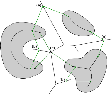
Figure 8. Types of linking for multi-region configuration in ${\mathbb{R}}^{2}$: a) linking between two objects; b) self-linking; and c) partial linking.

Remark 3.3.

If $\Omega_{i}$ and $\Omega_{j}$ share a common boundary region, then certain strata in $M_{i}$ and $M_{j}$ are linked via points in this boundary region, and for those $x\in M_{i}$, $\ell_{i}(x)=r_{i}(x)$; see Figure 7.

4. Blum Medial Linking Structure for a Generic Multi-Region Configuration

Blum Medial Axis for a Single Region with Smooth Generic Boundary

In the case of a single region $\Omega$ with smooth generic boundary $\mathcal{B}$, the Blum medial axis $M$ is a special example of a skeletal structure which has special properties for both the medial axis $M$ and the radial vector field $U$. The generic local structure of $M$ is given by normal forms defined in terms of properties of the family of distance-squared functions. This family is the restriction of the “distance-squared function”  $\sigma(x,u)=\|x-u\|^{2}$ on ${\mathbb{R}}^{n+1}\times{\mathbb{R}}^{n+1}$. We let $\rho=\sigma|(\mathcal{B}\times{\rm int}\,(\Omega))$. Then, the Blum medial axis $M$ is the Maxwell set of $\rho$, which is the set of $u\in{\rm int}\,(\Omega))$ at which the absolute minimum of $\rho(\cdot,u)$ occurs at multiple points or is a degenerate minimum.

To describe the generic structure of $M$, we begin by recalling a result of Mather. In [M2], Mather is concerned with determining the generic structure of the distance function $\delta(x)=\min_{y\in\mathcal{B}}\|x-y\|$ from points $x\in{\mathbb{R}}^{n+1}\backslash\mathcal{B}$ to $\mathcal{B}$. He gives such a classification theorem which for generic $\mathcal{B}$ with $n+1\leq 7$ gives the structure of $\delta$ off of a finite set of points. He excludes a finite set of points for two reasons, which he does not really explain in the paper. One is that his classification excludes the classification at critical points of $\delta$ on strata of $M$. The second is because for $n+1=7$ there can be isolated points where the structure theorem for generic germs in terms of versal unfoldings as explained below does not directly apply.

We begin our discussion of his results stated in a form where they yield the generic structure of $M$, but do not consider the structure of the global distance function $\delta$ to $\mathcal{B}$.

Structure of Maxwell Set Described by $\mathcal{R}^{+}$-Versal Unfoldings

At a point $u_{0}\in M$ of the Maxwell set, we let $S=\{x_{1},\dots,x_{k}\}\subset\mathcal{B}$ be the points with $r_{0}=\rho(x_{i})=\rho(x_{j})$ for all $1\leq i,j\leq k$, the minimum value for $\rho(\cdot,u_{0})$ and consider the multigerm $\rho:\mathcal{B}\times{\mathbb{R}}^{n+1},S\times\{u_{0}\}\to{\mathbb{R}},r_{0}$, We view the coordinates of $u$ as a set of parameters for $u\in{\rm int}\,(\Omega)\subset{\mathbb{R}}^{n+1}$. The mapping $\rho$ is an “unfolding”of the multigerm $\rho_{0}=\rho(\cdot,u_{0}):\mathcal{B},S\to{\mathbb{R}},r_{0}$ on the parameters $u$. Such multigerms and their unfoldings are studied using $\mathcal{R}^{+}$-equivalence of multigerms $\rho_{0}$ and $\rho_{1}$ via the action of the group of pairs $(\varphi,c)$ which consist of a multigerm of a diffeomorphism $\varphi:\mathcal{B},S\to\mathcal{B},S$ and constant $c\in{\mathbb{R}}$, so $\rho_{0}$ is $\mathcal{R}^{+}$-equivalent to $\rho_{1}=\rho_{0}\circ\varphi+c$ (or for unfoldings $\rho$, pairs $\Psi(x,u)=(\psi(x,u),\lambda(u)):\mathcal{B}\times{\mathbb{R}}^{n+1},S\times\{u_{0}\}\to\mathcal{B}\times{\mathbb{R}}^{n+1},S\times\{u_{0}\}$ and a smooth function germ $c(u)$ so that $\rho$ is $\mathcal{R}^{+}$-equivalent to $\rho\circ\Psi+c(u)$). Singularity theory applies to the classification of such multigerms and their unfoldings. Provided $\rho_{0}$ has “finite $\mathcal{R}^{+}$-codimension”in an appropriate sense, then there is an $\mathcal{R}^{+}$-versal unfolding which is a finite parameter unfolding which captures all possible unfoldings of $\rho_{0}$ up to $\mathcal{R}^{+}$-equivalence (this extends to multigerms Thom’s versal unfolding theorem for germs which he used in Catastrophe Theory [Th]). The minimum number of parameters needed for the versal unfolding is the $\mathcal{R}^{+}_{e}$-codimension of $\rho_{0}$. These results are discussed by Mather in [M2], and some details relating versality and transversality that were left out are treated in a more general context in e.g. [D6].

These are applied by Mather to classify the local structure of the Blum medial axis. We view $\Omega$ as the region enclosed by the boundary $\mathcal{B}=\varphi(X)$, for $\varphi:X\to{\mathbb{R}}^{n+1}$ a smooth embedding and $X$ a smooth compact $n$-manifold. Then, there is the following theorem of Mather [M2] which describes the generic properties of the Blum medial axis of $\Omega$. The notion of “genericity”will be explained in more detail in §13.

Theorem 4.1 (Generic Properties of the Blum Medial Axis).

If $n+1\leq 6$, there is an open dense set of embeddings $\varphi\in{\rm Emb}\,(X,{\mathbb{R}}^{n+1})$ such that for any finite subset $S\subset\mathcal{B}=\varphi(X)$ and $u\in M$, for which $x,x^{\prime}\in S$ satisfy $\rho(x,u)=\rho(x^{\prime},u)(=r)$, then the multigerm $\rho:\mathcal{B}\times{\rm int}\,(\Omega),S\times\{u\}\to{\mathbb{R}},r$ is a versal unfolding for $\mathcal{R}^{+}$-equivalence of multigerms.

If $n+1=7$, then there is a finite set of points $E_{M}\subset M$ which form strata of dimension $0$ such that for $u\in M\backslash E_{M}$ the same conclusions hold for multigerms of $\rho$; while for each point $u\in E_{M}$, there is a unique point $S=\{x\}$ in $\mathcal{B}$ and the unfolding $\rho$ at $(x,u)$ defines a transverse section to the $\tilde{E}_{7}$-stratum (see below).

Remark 4.2.

In the case $n+1=7$, there may be isolated points $u\in M$ with each having a unique corresponding point $x\in\mathcal{B}$ such that the germ of $\rho(\cdot,u)|\mathcal{B}$ at $x$ is $\mathcal{R}^{+}$–equivalent in local coordinates $(y_{1},\dots,y_{6})$ to an $\tilde{E}_{7}$ singularity $y_{1}^{4}+y_{2}^{4}+ay_{1}^{2}y_{2}^{2}+y_{3}^{2}+\cdots+y_{6}^{2}$, where $|a|<2$. However the corresponding unfolding is not $\mathcal{R}^{+}$–versal as $a$ is a modulus and the entire stratum in jet space formed by the $\mathcal{R}^{+}$–orbits allowing $a$ to vary has $\mathcal{R}^{+}$–codimension $7$, while the individual orbits have codimension $8$. Generically a germ in the stratum may occur at an isolated point; and the resulting unfolding cannot be versal but it does define a transverse section to the $\tilde{E}_{7}$-stratum.

Now such unfoldings of $\tilde{E}_{7}$ germs are understood by a result of Looijenga [L2], from which it follows that the topological classification of $M$ near such $\tilde{E}_{7}$ points is independent of $a$ for $|a|<2$. Moreover, it follows that the associated mappings used in Lemma 15.3 are topologically stable by Looijenga’s theorem using the argument in [D8, Thm. 4]. Thus, the arguments in §15 still can be applied when appropriately modified in neighborhoods of the $\tilde{E}_{7}$ points using topological stability. We refer to such points as generic $\tilde{E}_{7}$ points.

For $n+1\leq 7$, Mather’s theorem then gives the list of possible multigerms and hence the corresponding local structure of $M$ resulting from the normal forms for the versal unfolding, except at the finite set of points in $E_{M}$ when $n+1=7$.

Excluding the case of $E_{M}$ when $n+1=7$, since each germ represents a local minimum for points on the Blum medial axis, the only germs which occur are the $A_{k}$ singularities, which are $\mathcal{R}^{+}$-equivalent in local coordinates $(y_{1},\dots,y_{n})$ to $y_{1}^{k+1}+\sum_{j=2}^{n}y_{j}^{2}$ for $k$ odd. If $\rho(\cdot,u)$ is a germ of type $A_{\alpha_{j}}$ at the point $x_{j}$, then the multigerm is said to be of generic type $A_{\boldsymbol{\alpha}}$ where $\boldsymbol{\alpha}=(\alpha_{1},\dots,\alpha_{k})$, and is denoted $A_{\alpha_{1}}A_{\alpha_{2}}\cdots A_{\alpha_{k}}$ (where it is customary to denote $A_{\alpha_{i}}$ repeated $r$ times using exponent notation $A_{\alpha_{i}}^{r}$).

In the generic case, the set of points $u\in M$ of type $A_{\boldsymbol{\alpha}}$ forms a submanifold $\Sigma_{M}^{(\boldsymbol{\alpha})}$ whose codimension in ${\mathbb{R}}^{n+1}$ equals the $\mathcal{R}^{+}_{e}$ codimension of a multigerm of type $A_{\boldsymbol{\alpha}}$, which equals $|\boldsymbol{\alpha}|-1$, with $|\boldsymbol{\alpha}|=\sum_{i=1}^{k}\alpha_{j}$. In addition, the $\{\Sigma_{M}^{(\boldsymbol{\alpha})}:|\boldsymbol{\alpha}|\leq n+2\}$ form a Whitney stratification of $M$ (because by the versality theorem, the structure of $M$ is analytically trivial along the strata, while for different simple types the topological structure of the stratification differs). The smooth points of $M$ are the points $u$ where $\rho(\cdot,u)$ has an $A_{1}^{2}$ singularity. The singular strata are of two types. The stratum consisting of points $u$ with $\rho(\cdot,u)$ having a single $A_{3}$ singularity forms the edge of $M$, denoted $\partial M$. This is part of the boundary of the regular stratum viewed as an $n$-manifold. The closure $\overline{\partial M}$ consists of strata $\Sigma_{M}^{(\boldsymbol{\alpha})}$ with some $\alpha_{i}\geq 3$ (and in the case $n+1=7$ the $\tilde{E}_{7}$ germs). The second type of singular strata are the $A_{1}^{k}$ strata with $k>2$ which are interior strata. For ${\mathbb{R}}^{3}$ see Figure 9 and the accompanying Example 4.3.

Stratification of the Boundary $\mathcal{B}$

Mather does not explicitly refer to the stratification of the boundary. However, it plays an important role when we consider configurations of regions. Corresponding to each stratum $\Sigma_{M}^{(\boldsymbol{\alpha})}$ are strata of $\mathcal{B}$ consisting of the individual $x_{i}$ which belong to the subset $S$ defining points in $\Sigma_{M}^{(\boldsymbol{\alpha})}$, see Figures 9 and 10. We denote the corresponding strata of $\mathcal{B}$ by $\Sigma_{\mathcal{B}}^{(\boldsymbol{\alpha})}$. These strata are the images under projection onto $\mathcal{B}$ of strata in the space of the versal unfolding. In turn, those strata consist of subsets of points where the unfolding defines multigerms of a given type. However, the unfolding theorem does not assert that the strata in $\mathcal{B}$ need be smooth of the same dimension as corresponding strata in $M$. We shall later prove that generically the $\Sigma_{\mathcal{B}}^{(\boldsymbol{\alpha})}$ are indeed smooth submanifolds of the same dimension as $\Sigma_{M}^{(\boldsymbol{\alpha})}$. As $S$ and $\boldsymbol{\alpha}$ have no intrinsic ordering, when we refer to one of these strata in $\mathcal{B}$ which contains $x_{j}$ we shall place $\alpha_{j}$ first in the ordering. If $n+1=7$, there are unique generic $\tilde{E}_{7}$ points on $\mathcal{B}$ corresponding to each of (the finite number of) points of $E_{M}$; these form a set of $0$-dimensional strata $E_{\mathcal{B}}$.

Stratification of $\mathcal{B}$ by $\Sigma_{\mathcal{B}}^{(\boldsymbol{\alpha})}$:

The $\Sigma_{\mathcal{B}}^{(\boldsymbol{\alpha})}$ define a stratification of $\mathcal{B}$ which we may view as consisting of three parts:

1. The first part consists of edge closure points and has a Whitney stratification consisting of the strata $\Sigma_{\mathcal{B}}^{(\boldsymbol{\alpha})}$ containing the point $x_{1}$ with $\alpha_{1}\geq 3$. This is the subset of $\mathcal{B}$ where $\rho(\cdot,u)$ has a local minimum of Thom-Boardman type $\Sigma_{n,1}$ for some $u\in\Omega$; or if $n+1=7$, it also contains the $0$-dimensional strata $E_{\mathcal{B}}$.

2. The second part has a Whitney stratification consisting of the strata $\Sigma_{\mathcal{B}}^{(\boldsymbol{\alpha})}$ with all $\alpha_{i}=1$.

3. The third part consists of the $A_{1}$ points which belong to a tuple in $\Sigma_{\mathcal{B}}^{(\boldsymbol{\alpha})}$ with some $\alpha_{j}\geq 3$ for $j>1$ (thus, they are points associated via the medial axis to edge-closure points in the Blum medial axis).

Although we will only show that the first two of these subsets of strata each separately form Whitney stratifications, it should be possible with considerably more work to show that together they form a Whitney stratification of $\mathcal{B}$.

Example 4.3.

For a generic region in ${\mathbb{R}}^{2}$, the refinement of $\tilde{M}$ only involves adding a finite number of isolated points to smooth curve segments, so the stratification is Whitney. For a generic region in ${\mathbb{R}}^{3}$, the standard local Blum types are $A_{1}^{2}$, $A_{3}$, $A_{1}A_{3}$, $A_{1}^{3}$, and $A_{1}^{4}$ (the first consists of smooth points of $M$ and the others are shown in Figure 9). In Figure 10, we show the corresponding local stratification types for the boundary. The $A_{3}$ and $A_{3}A_{1}$ points correspond to the edge-closure points; the $A_{1}^{3}$ and $A_{1}^{4}$ points form the $A_{1}^{k}$-types, and the last $A_{1}$ point of type $A_{1}A_{3}$ is the third type. In this case, a direct calculation shows that the closure of the $A_{1}^{2}$ points at an $A_{3}A_{1}$ point in the boundary is a smooth curve, so that the $\Sigma_{\mathcal{B}}^{(\boldsymbol{\alpha})}$ form a Whitney stratification of $\mathcal{B}$.

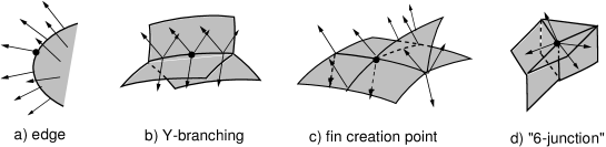
Figure 9. Generic local medial axis structures in ${\mathbb{R}}^{3}$: in a) the $A_{3}$ points form the edge curve and in b) the $A_{1}^{3}$ points form the “Y-branch curve”; for c) there is an isolated $A_{1}A_{3}$ point which is the fin point and for d), an isolated $A_{1}^{4}$ point which is the “$6$-junction”point.

Figure 10. Generic local stratification of the boundary $\mathcal{B}$ for a region in ${\mathbb{R}}^{3}$ in terms of the corresponding types on the medial axis listed in Figure 9 in terms of their $A_{\boldsymbol{\alpha}}$-type: $A_{3}$ and $A_{1}^{3}$ are the dimension $1$ strata in $\mathcal{B}$ corresponding to edge and $Y$-branching curves (with $3$ $A_{1}^{3}$ strata in the boundary for each $Y$-branching curve), while the other three are dimension $0$ strata of $\mathcal{B}$ corresponding to the $0$-dimensional strata of the medial axis in Figure 9; and the complement consists of open strata in $\mathcal{B}$ corresponding to the $2$-dimensional strata in the medial axis consisting of $A_{1}^{2}$ points. Note there are $4$ $A_{1}^{4}$ strata in the boundary for each $6$-junction point, and the last two figures represent strata on the two opposite boundary regions correponding to the “fin creation point”$A_{1}A_{3}$.

Addendum to Generic Blum Structure for a Region with Boundaries and Corners

There is an addendum to Mather’s theorem in the case of regions $\Omega$ which are manifolds with boundaries and corners. It concerns the local form of the Blum medial axis in a neighborhood of a $k$-edge-corner point for regions with boundaries and corners, which we introduced at the beginning of §2. This is described using the following normal form .

Definition 4.4.

The edge-corner normal form for the Blum medial axis of a $k$-edge-corner point $x$ consists of a smooth diffeomorphism $\psi$ from the neighborhood of $0$ in $C_{k}={\mathbb{R}}^{k}_{+}\times{\mathbb{R}}^{n+1-k}$, $k\geq 2$, to a neighborhood $W$ of $x$ with $0\mapsto x$ such that the medial axis in $W$ is the image $\psi(E)$, where

$$E_{k}=\{u=(u_{1},\dots,u_{n+1})\in C_{k}:\makebox{ there are $1\leq i,j\leq k$ such that $i\neq j$ and $u_{i}=u_{j}$}\}$$

with the canonical Whitney stratification of $E_{k}\cup\partial C_{k}$.

For example in ${\mathbb{R}}^{3}$, a) and b) of Figure 11 illustrate the edge-corner normal forms for the Blum medial axis at $P_{2}$ and $P_{3}$-edge-corner points.

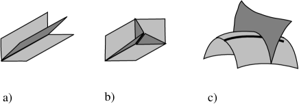
Figure 11. a) and b) edge corner normal forms for $P_{2}$ and $P_{3}$ points. The darker shaded regions are the Blum medial axis. c) Example at a $Q_{1}$ point of the transverse intersection of $\Sigma_{Q}$ with the $A_{3}$ curve in the boundary.

We use similar notation for Mather’s Theorem, where now $X$ is the boundary of the compact region $\Delta\subset{\mathbb{R}}^{n+1}$ which has boundaries and corners. In addition, for an embedding $\varphi:\Delta\to{\mathbb{R}}^{n+1}$, $\Omega=\varphi(\Delta)$ and $\mathcal{B}=\varphi(X)$. Then, the addendum is the following.

Theorem 4.5 (Addendum to Generic Properties of the Blum Medial Axis).

If $n+1\leq 7$, then there is an open dense set of embeddings $\varphi\in{\rm Emb}\,(\Delta,{\mathbb{R}}^{n+1})$, such that:

• the Blum medial axis has the same local properties in the interior of the region ${\rm int}\,(\Omega)$ as given in Theorem 4.1.

• if $n+1=7$, then at a point $u_{0}\in E_{M}$ with corresponding $x_{0}\in E_{\mathcal{B}}$, the unfolding germ $(x,u)\mapsto(\rho(x,u),u):\mathcal{B}\times{\rm int}\,(\Omega),(x_{0},u_{0})\to{\mathbb{R}}\times{\rm int}\,(\Omega)$ is a topologically stable unfolding of an $\tilde{E}_{7}$ germ;

• the set of closure points in the boundary $\mathcal{B}$ of the Blum medial axis consists of the edge-corner point strata of $\mathcal{B}$;

• at these edge-corner points, the Blum medial axis satisfies the edge-corner normal form.

For noncompact $\Omega$, the same result holds on a given compact region of ${\mathbb{R}}^{n+1}$ for an open dense set of embeddings.

If there is a compact Whitney stratified set $\mathcal{S}$ contained in the smooth strata of the boundary, then for an open dense set of embeddings, the strata of $\mathcal{S}$ are transverse to the strata $\Sigma_{\mathcal{B}}^{(\boldsymbol{\alpha})}$.

This addendum will be proved in the process of establishing the generic Blum structure for general multi-region configurations (Theorem 4.18) in §15. The specific information about $E_{M}$ follows using a result of Looijenga [L2] and is explained in §15.

Remark 4.6.

The Blum medial structure $M$ for a region with boundary and corners contains the singular points of the boundary in its closure, and at such points the radial vector field $U=0$. Hence, $(M,U)$ does not define a skeletal structure in the strict sense. However, it can still be used in exactly the same way to compute the local, relative, and global geometry and topology of both the region and its boundary, just as for skeletal structures. Hence, we can view it as a “relaxed skeletal structure”, where “relaxed”means that $M$ includes the singular boundary points and $U=0$ on these points.

Spherical Axis of a Configuration

Along with the medial axis, we will also find use for its analog for the family of height functions. This family is the restriction of the “height function”  $\nu:{\mathbb{R}}^{n+1}\times S^{n}\to{\mathbb{R}}$, defined by $\nu(x,v)=x\cdot v$, to $\tau:\mathcal{B}\times S^{n}\to{\mathbb{R}}$ ($S^{n}$ is the unit sphere in ${\mathbb{R}}^{n+1}$). Here $\mathcal{B}$ may denote the smooth generic boundary of a single region $\Omega$, or more generally the boundary for a configuration defined by $\Phi:\boldsymbol{\Delta}\to{\mathbb{R}}^{n+1}$. We define the spherical axis $\mathcal{Z}\subset S^{n}$ of $\Omega$ or the configuration $\boldsymbol{\Omega}$ defined by $\Phi$ to be the Maxwell set of $-\tau$, which is the set of $v\in S^{n}$ at which the absolute maximum of $\tau(\cdot,v)$ occurs at multiple points or is a degenerate maximum. This consists of directions $v\in S^{n}$ for which the supporting hyperplanes $x\cdot v=c$ for the convex hull of $\Omega$ or $\boldsymbol{\Omega}$ have more than two tangencies with $\mathcal{B}$ or a degenerate tangency, (and $v$ is normal to $\mathcal{B}$ at these points) see e.g. Figure 13. Recall that $x\cdot v=c$ defines a supporting hyperplane for $\boldsymbol{\Omega}$ if it meets the boundary $\mathcal{B}$ of $\boldsymbol{\Omega}$, which is contained in the half-space defined by $x\cdot v\leq c$.

Remark 4.7.

We note that while the height function depends on the choice of the origin, the spherical axis doesn’t. Choosing a different point for the origin only changes the height function by adding a constant. This will not change which points on $\mathcal{B}$ are critical points, nor which type of singularity occurs at these critical points. If there are multiple critical points at the same “height”, they will remain at the same height when we shift the point (but the height will change by the same amount for all).

Then, there is the following analog of the addendum to Mather’s Theorem.

Theorem 4.8 (Generic Properties of the Spherical Axis).

If $n+1\leq 7$, there is an open dense set of embeddings of configurations $\Phi\in{\rm Emb}\,(\boldsymbol{\Delta},{\mathbb{R}}^{n+1})$ such that for any finite subset $S\subset\mathcal{B}$ and $v\in M$, for which $x,x^{\prime}\in S$ satisfy $\tau(x,v)=\tau(x^{\prime},v)(=r)$, then the multigerm $\tau:\mathcal{B}\times S^{n},S\times\{v\}\to{\mathbb{R}},r$ is a versal unfolding for $\mathcal{R}^{+}$-equivalence of multigerms.

If $n+1=8$, then there is a finite set $E_{\mathcal{Z}}\subset\mathcal{Z}$ such that for any $v\in\mathcal{Z}\backslash E_{\mathcal{Z}}$, the same conclusions hold for the multigerms of $\tau$; while at points $v\in E_{\mathcal{Z}}$, $\tau$ has a generic $\tilde{E}_{7}$ singularity.

This result will follow from the transversality results in Proposition 14.8 as explained in §14.

Note: this holds for $n+1\leq 8$, because the dimension of the parameter space $S^{n}$ is one less than that of ${\mathbb{R}}^{n+1}$. This again gives the list of possible multigerms and hence the corresponding local structure of $M$ resulting from the normal forms for the versal unfolding. Again since each germ for points on the spherical axis represents a local minimum of $-\tau$ (or local maximum for $\tau$), the only germs which occur are the $A_{k}$ singularities, for $k$ odd, which are local minima (or local maxima for $\tau$).

In the generic case, it follows that the set of points $v\in\mathcal{Z}$ of type $A_{\boldsymbol{\alpha}}$ forms a submanifold $\Sigma_{\mathcal{Z}}^{(\boldsymbol{\alpha})}$ whose codimension in $S^{n}$ equals the $\mathcal{R}^{+}_{e}$ codimension of a multigerm of type $A_{\boldsymbol{\alpha}}$. In addition, the $\{\Sigma_{\mathcal{Z}}^{(\boldsymbol{\alpha})}:|\boldsymbol{\alpha}|\leq n+1\}$ form a Whitney stratification of $\mathcal{Z}$. This stratification has the same generic form as for the Blum medial axis except for one lower dimension.

Spherical Structure for a Configuration

Just as for the Blum medial axis, we may associate to the spherical axis $\mathcal{Z}$, both a height function $h$ and a multivalued vector field $V$. To do this we need to initialize the origin. Then, the height for a point $\mathbf{u}$ on the spherical axis, which is a unit vector, defined for a point $x\in\mathcal{B}$ is just the dot product $x\cdot\mathbf{u}$. Furthermore, there may be multiple points associated to $\mathbf{u}$, all of which lie in the supporting hyperplane $H$ defined by $x\cdot\mathbf{u}=h(\mathbf{u})$, for the maximum value $h=h(\mathbf{u})$ for $\mathcal{B}$. For each point $x_{i}\in H\cap\mathcal{B}$, there is a vector $V=x_{i}-h\mathbf{u}$ orthogonal to the line spanned by $\mathbf{u}$. This defines a multivalued vector field $V$.

Definition 4.9.

The full spherical structure for the spherical axis of the multi-region configuration is the triple $(\mathcal{Z},h,V)$, consisting of the spherical axis $\mathcal{Z}$, the height function $h$, and the multivalued vector field $V$. This depends upon the choice of an origin on which all height functions are $0$.

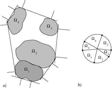
Figure 12. a) Configuration of four regions with the bitangent supporting lines, and b) the corresponding spherical axis, which consists of the points on $S^{1}$. The regions between points represent subregions of $\mathcal{B}$ in $\mathcal{B}_{\infty}$. If the same region $\Omega_{i}$ is indicated on both sides of a radial line, then in $\mathcal{B}_{i}$ is a region involving self-linking.

From the spherical structure, we can reconstruct the boundary of $\mathcal{B}_{\infty}$ by $x=V(\mathbf{u})+h(\mathbf{u})\mathbf{u}$ for $\mathbf{u}\in\mathcal{Z}$ and the multiple values of $V$ at $\mathbf{u}$. Here $x$ denotes a collection of points corresponding to the values of $V$.

Then, the regions in ${\rm int}\,(\mathcal{B}_{\infty})$ are the regions in the complement of the boundary of $\mathcal{B}_{\infty}$ which have supporting hyperplanes for at least one point in one of the corresponding complementary regions to the spherical axis. If we have in addition the height function for the configuration defined on all of $S^{n}$, then we can construct the supporting hyperplanes for all $\mathbf{u}\in S^{n}$, and the envelope of these hyperplanes yields $\mathcal{B}_{\infty}$.

Example 4.10.

For generic configurations in ${\mathbb{R}}^{2}$, the spherical axis consists of a finite number of points in $S^{1}$ representing bitangent supporting lines. This is illustrated in Figure 12.

In the case of generic configurations in ${\mathbb{R}}^{3}$, the spherical axis consists of curve segments which may either end or three may join at a “$Y$-branch point”. These curves divide the complement in $S^{2}$ into connected components which correspond to regions of the $\mathcal{B}_{i}$ which will not be linked in the Blum case to follow. In Figure 13 are illustrated the three configurations in ${\mathbb{R}}^{3}$ which exhibit the basic properties for the spherical axis: a) smooth curve segment, b) $Y$-branch point, and c) end point at an $A_{3}$ singularity.

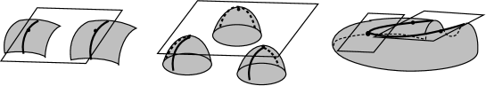
a)                        b)                                   c)

Figure 13. The generic multigerms for the height function. These determine the local structure for the boundary strata of $M_{\infty}$ for a multi-region configuration in ${\mathbb{R}}^{3}$ : a) of type $A_{1}^{2}$, b) of type $A_{1}^{3}$, and c) of type $A_{3}$. The tangent planes shown are to points of multiple tangencies (except for the single $A_{3}$ point on the left in c). The darker curves (including the darker dashed curves) denote the boundary strata bounding regions of $M_{\infty}$ (consisting of points whose outward pointing normals point away from the other regions).

Blum Medial Linking Structure

We now consider the analogous Blum medial linking structure for a generic multi-region configuration. First, we note that if the configuration has regions with boundaries and corners, then the Blum medial axes of the individual regions will not define skeletal structures. This is because the Blum medial axis will actually meet the boundary at the edges and corners. However, in the case of disjoint regions $\{\Omega_{i}\}$ in ${\mathbb{R}}^{n+1}$ with smooth generic boundaries (which do not intersect on their boundaries) there is a natural Blum version of a linking structure, which we introduce.

Definition 4.11.

Given a multi-region configuration of disjoint regions $\boldsymbol{\Omega}=\{\Omega_{i}\}$ in ${\mathbb{R}}^{n+1}$, for $i=1,\dots,m$, with smooth generic boundaries (which do not intersect on their boundaries), a Blum medial linking structure is a skeletal linking structure for which:

• the $M_{i}$ are the Blum medial axes of the regions $\Omega_{i}$ with $U_{i}$ the corresponding radial vector fields;

• the linking axis $M_{0}$ is the Blum medial axis of the exterior region $\Omega_{0}$; and

• $M_{i\,\infty}$, which consists of the points in $\tilde{M}_{i}$ which are unlinked to any other points, corresponds to the points in $\mathcal{B}_{i\,\infty}\subset\mathcal{B}_{i}$ for which a height function has an absolute maximum on $\mathcal{B}$ (or minimum for the height function for the opposite direction).

Because of B2), we will frequently in the Blum case refer to $M_{0}$ as the linking medial axis.

Remark 4.12.

It follows from B2) that if $x\in M_{i}$ and $x^{\prime}\in M_{j}$ are linked, the corresponding values of the radial and linking functions satisfy $\ell_{i}(x)-r_{i}(x)=\ell_{j}(x^{\prime})-r_{j}(x^{\prime})$.

Generic Linking Properties

Consider a configuration $\{\Omega_{i}\}$ with $\mathcal{B}_{i}$ the boundary of $\Omega_{i}$, and $M_{i}$ the Blum medial axis of $\Omega_{i}$. We let $\mathcal{B}=\cup\mathcal{B}_{i}$ and let $\sigma(x,u)=\|x-u\|^{2}$ denote the distance squared function on ${\mathbb{R}}^{n+1}\times{\mathbb{R}}^{n+1}$ as earlier. We consider a collection of smooth boundary points $S=\{x_{1},\dots,x_{r}\}$ with $x_{i}\in\mathcal{B}_{j_{i}}$.

Definition 4.13.

The set of points $S=\{x_{1},\dots,x_{r}\}$ exhibits generic Blum linking of type $(A_{\boldsymbol{\alpha}}:A_{\boldsymbol{\beta}_{1}},\dots,A_{\boldsymbol{\beta}_{r}})$ if:

• there is a $u_{0}\in\Omega_{0}$ so that $\sigma(\cdot,u_{0})|\mathcal{B}$ has a common minimum on $S$ with value $\sigma(x_{i},u_{0})=y_{0}$, and $\sigma:\mathcal{B}\times{\mathbb{R}}^{n+1},(S,w)\rightarrow{\mathbb{R}},y_{0}$ is of generic type $A_{\boldsymbol{\alpha}}$;

• for each $i$, there is a subset $S_{i}\subset\mathcal{B}_{j_{i}}$ and a point $u_{i}\in M_{i}$, so that $\sigma(\cdot,u_{i})|\mathcal{B}_{j_{i}}$ has a common minimum on $S_{i}$ with value $r_{i}$ and $\sigma:\mathcal{B}\times{\mathbb{R}}^{n+1},S_{i}\times\{u_{i}\}\to{\mathbb{R}},r_{i}$ is of generic type $A_{\boldsymbol{\beta}_{i}}$;

• the singular sets $\Sigma_{\mathcal{B}}^{(\boldsymbol{\alpha})}\subset\mathcal{B}$ and $\Sigma_{\mathcal{B}_{j_{i}}}^{(\boldsymbol{\beta}_{i})}\subset\mathcal{B}_{j_{i}}$ intersect transversely in $\mathcal{B}_{j_{i}}$; and

• the images of the strata $\Sigma_{\mathcal{B}}^{(\boldsymbol{\alpha})}\cap\Sigma_{\mathcal{B}_{j_{i}}}^{(\boldsymbol{\beta}_{i})}$ in $\Sigma_{M_{0}}^{(\boldsymbol{\alpha})}$ intersect in general position.

If $n+1=7$, then we may also have generic Blum linking involving generic $\tilde{E}_{7}$ points for either self-linking $(\tilde{E}_{7}:A^{2}_{1})$ or simple linking $(A^{2}_{1}:\tilde{E}_{7},A^{2}_{1})$.

We will often abbreviate the above notation with $\boldsymbol{\beta}=\{\boldsymbol{\beta}_{1},\dots,\boldsymbol{\beta}_{r}\}$, by $(A_{\boldsymbol{\alpha}}:A_{\boldsymbol{\beta}})$. For a given $(\boldsymbol{\alpha}:\boldsymbol{\beta})$, we let $\Sigma_{M_{0}}^{(\boldsymbol{\alpha}:\boldsymbol{\beta})}$ denote the set of points $u_{0}\in\Omega_{0}$ exhibiting the properties in i) - iv) in Definition 4.13. We shall prove that it is a smooth submanifold of the stratum $\Sigma_{M_{0}}^{(\boldsymbol{\alpha})}$ of the Blum medial axis $M_{0}$ of $\Omega_{0}$. Along with the stratum $\Sigma_{M_{0}}^{(\boldsymbol{\alpha}:\boldsymbol{\beta})}$, we also have the corresponding stratum $\Sigma_{\mathcal{B}_{j_{i}}}^{(\boldsymbol{\alpha}:\boldsymbol{\beta})}\subset\mathcal{B}_{j_{i}}$ consisting of those points $x_{j_{i}}\in\Sigma_{\mathcal{B}_{j}}^{(\boldsymbol{\beta}_{i})}$ which correspond to points in $\Sigma_{M_{0}}^{(\boldsymbol{\alpha}:\boldsymbol{\beta})}$. We shall prove for a generic configuration, that the $\{\Sigma_{\mathcal{B}_{j}}^{(\boldsymbol{\alpha}:\boldsymbol{\beta})}\}$ give a refinement of the stratification of $\mathcal{B}_{j}$ by the $\{\Sigma_{\mathcal{B}_{j}}^{(\boldsymbol{\beta}_{i})}\}$, and $\{\Sigma_{M_{0}}^{(\boldsymbol{\alpha}:\boldsymbol{\beta})}\}$ gives a refinement of the Whitney stratification of $M_{0}$.

For a given $\mathcal{B}_{j}$ we may divide the strata into groups based on whether for $x_{j\,1}\in\mathcal{B}_{j}$, $\alpha_{j}\geq 3$ or $\alpha_{i}=1$ for all $i$ and whether $\beta_{j\,1}\geq 3$ or $\beta_{j\,i}=1$ for all $i$. The intersection of the strata for each of the pairs of groups will satisfy the Whitney conditions. In the low dimensional cases of multi-region configurations in ${\mathbb{R}}^{2}$ or ${\mathbb{R}}^{3}$, the $\Sigma_{\mathcal{B}_{j}}^{(\boldsymbol{\alpha}:\boldsymbol{\beta})}$ give a Whitney stratification of $\mathcal{B}_{j}$.

For a configuration in ${\mathbb{R}}^{3}$ the stratifications of a boundary $\mathcal{B}_{j}$ given by either $\Sigma_{\mathcal{B}_{j}}^{(\boldsymbol{\alpha})}$ or $\Sigma_{\mathcal{B}_{j}}^{(\beta_{j})}$ locally have the forms in Figure 10. Their transverse intersection implies that $0$ dimensional strata of one will lie in a smooth strata of the other. Also, the $1$ dimensional strata will intersect transversally giving four possibilities. For a point in one of these intersections, any other point in another $\mathcal{B}_{i}$ associated to the corresponding point in $\Sigma_{M_{0}}^{(\boldsymbol{\alpha})}$ must be of type $A_{1}^{2}$ by property iv) of Definition 4.13. If instead the point in $\Sigma_{M_{0}}^{(\boldsymbol{\alpha})}$ is in a singular stratum of dimension $0$, then all associated points in some $\mathcal{B}_{i}$ are of type $A_{1}^{2}$. A third possibility for a smooth point of $M_{0}$, which is an $A_{1}^{2}$ point for say $\mathcal{B}_{i}$ and $\mathcal{B}_{j}$, is that the images of the corresponding $1$-dimensional strata $\Sigma_{\mathcal{B}_{i}}^{(\beta_{i})}$ and $\Sigma_{\mathcal{B}_{j}}^{(\beta_{j})}$ intersect transversally in a smooth point of $M_{0}$. This gives a corresponding analysis. Together these yield all of the generic linking types listed in Table LABEL:Table1 in the Addendum.

Examples of some linking types and the strata are illustrated in Figure 14.

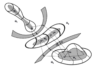
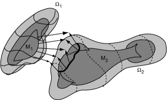
a)                                                         b)

Figure 14. Examples of linking types. In a) points (a) and (b) illustate linking of type $(A_{1}^{2}:A_{3},A_{3})$, and (c) of type $(A_{1}^{2}:A_{3}A_{1},A_{1}^{2})$. In b) is illustrated via the dark curve consisting of $1$-dimensional strata of type $(A_{1}^{2}:A_{3},A_{1}^{2})$ and isolated points of types $(A_{1}^{2}:A_{3},A_{1}^{3})$ and $(A_{1}^{2}:A_{3},A_{3})$ where the curve crosses the $Y$-branch curve of the medial axis $M_{2}$ of $\Omega_{2}$, resp. where it meets the edge of $M_{2}$.

Remark 4.14.

For a general multi-region configuration, we can substitute in place of $\Omega_{0}$ a region $\Omega_{i}$ which has multiple adjoining regions (including possibly the complement $\Omega_{0}$) and the definition of “generic linking”of the adjoining regions relative to $\Omega_{i}$ has the same form as in Definition 4.13. We shall see that generically they have the same properties as for $\Omega_{0}$.

If we consider the double $\tilde{M}_{i}$, only part of the stratification of $M_{i}$ coming from one side of $\Omega_{i}$ appears and this simplifies the resulting stratification of $\tilde{M}_{i}$. Only for the complement $\Omega_{0}$ and $M_{0}$ does the stratification of $M_{0}$ itself play an important role.

Generic Structure for $\mathcal{B}_{\infty}$ and $M_{\infty}$

We recall that $\mathcal{B}_{\infty}$ and $M_{\infty}$ denote the unions of the $\mathcal{B}_{i\,\infty}$, respectively $M_{i\,\infty}$. We will show in the generic case for $n+1\leq 7$ that the stratification of $\mathcal{B}_{\infty}$ has the following properties. The interior points of $\mathcal{B}_{i\,\infty}$ are those points where a height function has a unique absolute minimum on $\mathcal{B}$. In addition, the boundary of $\mathcal{B}_{i\,\infty}$ consists of strata $\Sigma^{(\boldsymbol{\alpha})}_{\infty}$ defined by the $\mathcal{R}^{+}$- versal unfolding of a multigerm of the height function of type $\mathbf{A}_{\boldsymbol{\alpha}}$ of $\mathcal{R}^{+}_{e}$–codimension $\leq n$. These strata lie in the smooth strata of the $\mathcal{B}_{i}$ and correspond to the strata $\Sigma^{(\boldsymbol{\alpha})}_{\mathcal{Z}}$ of the spherical axis $\mathcal{Z}$ and are of the same dimensions. The strata $\Sigma^{(\boldsymbol{\alpha})}_{\infty}$ again forms a collection of three stratifications with the same properties listed for the distance function for types 1) - 3). For ${\mathbb{R}}^{2}$ and ${\mathbb{R}}^{3}$, these together form Whitney stratifications for $\mathcal{B}_{\infty}$ for elementary reasons.

Furthermore, we will show that generically this stratification intersects tranversally the stratification $\Sigma^{(\boldsymbol{\beta})}_{\mathcal{B}_{i}}$ for the Blum medial axis of $\Omega_{i}$. Then, the strata of $M_{\infty}$ are the images in $\tilde{M}_{i}$ of the transverse intersections $\Sigma^{(\boldsymbol{\alpha})}_{\infty}\cap\Sigma^{(\boldsymbol{\beta})}_{\mathcal{B}_{i}}$.

Definition 4.15.

By $M_{\infty}$ and $\mathcal{B}_{\infty}$ having generic structure we mean that each $\mathcal{B}_{i\,\infty}$ has the above local structure with the resulting generic structure for each $M_{i\,\infty}$.

Remark 4.16.

In the Blum case for disjoint regions with smooth boundaries, if we remove the self-linking set from the external linking axis, then we obtain what is classically called the “conflict set”, see e.g. Siersma[Si], Sotomayor-Siersma-Garcia[SSG], and Van Manen [VaM].

Existence of a Blum Medial Linking Structure

We use the notation of §2 and consider a model configuration $\boldsymbol{\Delta}$ but with the $\Delta_{i}$ disjoint regions with smooth boundaries $X_{i}$. Then, we let $\boldsymbol{\Omega}$ be a configuration based on $\boldsymbol{\Delta}$ via the embedding $\varphi:\boldsymbol{\Delta}\to{\mathbb{R}}^{n+1}$ so that $\Omega_{i}=\varphi(\Delta_{i})$ for each $i$ (in this case each $\Gamma_{i}=\Omega_{i}$). As earlier, the space of configurations of type $\boldsymbol{\Delta}$ is given by the space of embeddings ${\rm Emb}\,(\boldsymbol{\Delta},{\mathbb{R}}^{n+1})$.

Then, the existence of Blum medial linking structures is guaranteed by the following, which in addition ensures generic linking (see also [Ga]).

Theorem 4.17 (Existence of Blum Medial Linking Structure).

For $n+1\leq 7$, we consider multi-region configurations $\boldsymbol{\Omega}$ modeled by $\boldsymbol{\Delta}=\{\Delta_{i}\}$, consisting of disjoint regions with smooth boundaries (which do not intersect on their boundaries). Then, for any compact region $\tilde{\Omega}\subset{\mathbb{R}}^{n+1}$ with nonempty interior, there is an open dense set of embeddings $\Phi\in{\rm Emb}\,(\boldsymbol{\Delta},{\rm int}\,(\tilde{\Omega}))$ such that :

1. the resulting configuration $\{\Omega_{i}=\Phi(\Delta_{i})\}$ has a Blum medial linking structure such that each $M_{i}$ (including $M_{0}$) has generic local properties given by Theorem 4.1;

2. the linking structure exhibits generic linking as in Definition 4.13; and

3. $M_{\infty}$ and $\mathcal{B}_{\infty}$ have generic structure as given in Definition 4.15.

4. In the case that $\tilde{\Omega}$ is convex, the properties for a linking structure in the bounded case hold.

We shall prove Theorem 4.17 as a special case of the following more general genericity result for the full Blum linking structure for a multi-region configuration.

Theorem 4.18 (Full Blum Linking Structures).

For $n+1\leq 7$, let $\boldsymbol{\Delta}=\{\Delta_{i}\}$ be a model multi-region configuration. For a compact region $\tilde{\Omega}\subset{\mathbb{R}}^{n+1}$ with nonempty interior, there is an open dense set of embeddings $\Phi\in{\rm Emb}\,(\boldsymbol{\Delta},{\rm int}\,(\tilde{\Omega}))$ such that the resulting configuration $\boldsymbol{\Omega}$ modeled by $\boldsymbol{\Delta}$, with $\{\Omega_{i}(=\varphi(\Delta_{i}))\}$, has the following properties:

• each $\Omega_{i}$ has a Blum medial axis $M_{i}$ exhibiting the generic local properties in ${\rm int}\,(\Omega_{i})$ given by Theorem 4.17;

• the complement $\Omega_{0}$ exhibits the generic local properties on $M_{0}$ in ${\rm int}\,(\Omega_{0})\cap\tilde{\Omega}$;

• the local structure of $M_{i}$ (including $i=0$) near a boundary point of type $P_{k}$ or singular $Q_{k}$ point has the local generic edge-corner normal form given by Definition 4.4;

• at a smooth $Q_{k}$ boundary point of a region $\Omega_{i}$, $\Sigma_{Q\,i}$ intersects the strata $\Sigma_{\mathcal{B}_{i}}^{(\boldsymbol{\alpha}:\boldsymbol{\beta})}$ transversally (and if $n+1=7$ it does not contain $\tilde{E}_{7}$ points);

• generic linking occurs between the smooth points of the regions and no linking occurs at edge-corner points, and this holds as well for generic linking between adjoining regions of a given region $\Omega_{i}$ relative to the region $\Omega_{i}$; and

• $\mathcal{B}_{i\,\infty}$ is contained in the smooth strata of the $\mathcal{B}_{i}$ (as a piecewise smooth manifold), and $\mathcal{B}_{i\,\infty}$ and the corresponding strata of $M_{i\,\infty}$ exhibit the generic properties given in Definition 4.15.

The last two parts of this paper will be devoted to developing the necessary transversality theorems, associated computations, and auxiliary results for proving this theorem.

Remark 4.19.

For a bounded region $\tilde{\Omega}$ whose boundary $\partial\tilde{\Omega}$ is transverse to the linking vectors of $M_{0}$ (i.e. the extension of the radial lines from $M_{\infty}$ are tranverse to the limiting tangent spaces at points of $\partial\tilde{\Omega}$), we can modify the linking vectors that extend beyond $\tilde{\Omega}$, or the extension of the radial vectors from $M_{\infty}$, by truncating them at $\partial\tilde{\Omega}$. They will be stratawise smooth when we add the strata corresponding to the intersection $M_{0}\cap\partial\tilde{\Omega}$. For example if $\tilde{\Omega}$ is convex, then, for almost all small translations of the configuration, the resulting $M_{0}$ is transverse to $\partial\tilde{\Omega}$.

An alternate approach for a more general region $\tilde{\Omega}$ is to let the exterior region be $\Omega_{0}\cap\tilde{\Omega}$ and allow linking from $\partial\tilde{\Omega}$ with the other internal regions. Then, including $\tilde{\Omega}$ as part of the configuration, we may apply the existence theorem to give the result.

As an example, c) of Figure 11 illustrates iv) of the Theorem. By property iii) we see that the intersection of the closure of $M_{i}$ with the boundary consists of the singular points on the boundary. This holds equally well for the complement with the closure of $M_{0}$ containing the singular strata of the $\Gamma_{i}$ in ${\rm int}\,(\Omega_{0})\cap\tilde{\Omega}$.

One consequence of the characterization of generic linking in terms of the versality of the distance functions from Theorem 4.1 and the transversality of the stratifications is the determination of the codimensions of the strata.

Corollary 4.20.

For a generic embedding $\Phi:\boldsymbol{\Delta}\to{\mathbb{R}}^{n+1}$ as in Theorems 4.17 or 4.18, for $(\boldsymbol{\alpha}:\boldsymbol{\beta}_{1},\dots,\boldsymbol{\beta}_{r})$, the codimensions of the strata $\Sigma_{\mathcal{B}_{i}}^{(\boldsymbol{\alpha}:\boldsymbol{\beta})}$ and $\Sigma_{M_{i}}^{(\boldsymbol{\alpha}:\boldsymbol{\beta})}$ satisfy

(4.1) $${\rm codim}\,_{\mathcal{B}_{i}}(\Sigma_{\mathcal{B}_{i}}^{(\boldsymbol{\alpha}:\boldsymbol{\beta})})\,\,=\,\,{\rm codim}\,_{{\mathbb{R}}^{n+1}}(\Sigma_{M_{i}}^{(\boldsymbol{\alpha}:\boldsymbol{\beta})})\,-\,1,$$

and

(4.2) $${\rm codim}\,_{{\mathbb{R}}^{n+1}}(\Sigma_{M_{i}}^{(\boldsymbol{\alpha}:\boldsymbol{\beta})})\,\,=\,\,\mathcal{R}_{e}^{+}\text{- }{\rm codim}\,(\mathbf{A}_{\boldsymbol{\alpha}})\,+\,\sum_{p=1}^{r}\mathcal{R}_{e}^{+}\text{-}{\rm codim}\,(\mathbf{A}_{\boldsymbol{\beta}_{j_{p}}})\,-\,r.$$

This will be derived in §14.

As a consequence of the corollary, we can immediately list the generic linking types which can occur for a given ${\mathbb{R}}^{n+1}$ as ${\rm codim}\,(\Sigma_{M_{i}}^{(\boldsymbol{\alpha}:\boldsymbol{\beta})})\leq n+1$.

Addendum: Classification of Linking Types for Blum Medial Linking Structures in ${\mathbb{R}}^{3}$

For a generic configuration $\boldsymbol{\Omega}$ in ${\mathbb{R}}^{3}$, the Blum medial linking structure exhibits generic linking properties given by the Table LABEL:Table1. We first briefly explain the features of the table. Dimension refers to the dimension in ${\mathbb{R}}^{3}$ of the strata where the given linking type occurs. There are three types of linking: 1) linking between points on distinct medial axes; “partial linking”  involving more than one point from one medial axis and point(s) from another; and 3) “self-linking”  where linking is between points from a single medial axis. “Pure linking type”  refers to cases only occurring for self linking. The $A_{1}^{2}$ and $A_{1}A_{3}$ linking can occur for either linking or self-linking; while $A_{1}^{3}$ and $A_{1}^{4}$ linking can occur for any of the three linking types.

Table 1. Classification of Linking Types for Blum Medial Linking Structures in ${\mathbb{R}}^{3}$

	Linking Type	Dimension	Description of Linking
	$A_{1}^{2}$ Linking
i)	$(A_{1}^{2}:A_{1}^{2},A_{1}^{2})$	2	between $2$ smooth points
ii)	$(A_{1}^{2}:A_{1}^{3},A_{1}^{2})$	1	between a smooth point
			and a Y-junction point
iii)	$(A_{1}^{2}:A_{3},A_{1}^{2})$	1	between a smooth point
			and an edge point
iv)	$(A_{1}^{2}:A_{3}A_{1},A_{1}^{2})$	0	between a fin point
			and a smooth point
v)	$(A_{1}^{2}:A_{1}A_{3},A_{1}^{2})$	0	between a smooth point
			associated to a fin point and
			another smooth point
vi)	$(A_{1}^{2}:A_{1}^{4},A_{1}^{2})$	0	between a smooth point
			and a $6$-junction point
vii)	$(A_{1}^{2}:A_{1}^{3},A_{1}^{3})$	0	between $2$ Y-junction points
viii)	$(A_{1}^{2}:A_{3},A_{3})$	0	between $2$ edge points
ix)	$(A_{1}^{2}:A_{1}^{3},A_{3})$	0	between a Y-junction point
			and an edge point
	$A_{1}^{3}$, $A_{1}^{4}$ and $A_{1}A_{3}$ Linking
x)	$(A_{1}^{3}:A_{1}^{2},A_{1}^{2},A_{1}^{2})$	1	between $3$ smooth points
xi)	$(A_{1}^{3}:A_{1}^{3},A_{1}^{2},A_{1}^{2})$	0	between $2$ smooth points
			and a Y-junction point
xii)	$(A_{1}^{3}:A_{3},A_{1}^{2},A_{1}^{2})$	0	between $2$ smooth points
			and an edge point
xiii)	$(A_{1}^{4}:A_{1}^{2},A_{1}^{2},A_{1}^{2},A_{1}^{2})$	0	between $4$ smooth points
xiv)	$(A_{1}A_{3}:A_{1}^{2},A_{1}^{2})$	0	$A_{1}A_{3}$ linking between $2$
			smooth points
	Pure Self-Linking
xv)	$(A_{3}:A_{1}^{2})$	1	edge-type self-linking with
			a smooth point
xvi)	$(A_{3}:A_{1}^{3})$	0	edge-type self-linking with
			a Y-junction point
xvii)	$(A_{3}:A_{3})$	0	edge-type self-linking with
			an edge point

5. Retracting the Full Blum Medial Structure to a Skeletal Linking Structure

We know by Theorem 4.18 that a generic multi-region configuration has a Blum medial structure. If the regions are disjoint with smooth boundaries, then the Blum linking structure is a skeletal linking structure. However, if the configuration contains regions which adjoin, then the Blum linking structure does not satisfy all of the conditions for being a skeletal linking structure. Specifically the individual Blum medial axes of both the regions and the complement will extend to the singular points of the boundaries.

There are two perspectives on this. On the one hand, as mentioned in 4.6, we may view this as a “relaxed form of a skeletal linking structure”. We shall see that from this structure we still obtain all of the local, relative, and global geometry of the individual regions and the positional geometry of the configuration. However, if we consider the stability and deformation properties, such a structure does not behave well.

There are two approaches to modifying the full Blum linking structure to a skeletal linking structure. One approach is when the configuration with adjoined regions can be viewed as a deformation of a configuration with disjoint regions. The second is to modify the full Blum linking structure by a process of “smoothing the corners”of the regions. We consider each of these.

Example of Evolving Skeletal Linking Structure for Simple Generic Transition

We will not attempt to handle the most general case but illustrate the method for an adjoining of two regions. We assume that initially we have a configuration of two disjoint compact regions $\Omega_{i}$ in ${\mathbb{R}}^{n+1}$ with smooth boundaries $\mathcal{B}_{i}$ defined by the model $\Phi:\boldsymbol{\Delta}\to{\mathbb{R}}^{n+1}$. We consider a simple generic transition in the configuration defined by a smooth map $\Psi:\boldsymbol{\Delta}\times[0,1]\to{\mathbb{R}}^{n+1}$, with $\Psi_{0}=\Phi$, where disjoint regions becoming adjoined causes a transition in the full Blum medial linking structure as in Figure  15.

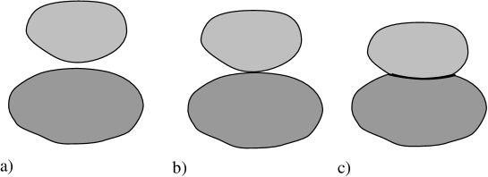
Figure 15. The stages for a simple generic transition of two evolving regions $\Omega^{\prime}_{i\,t}$ becoming adjoined: a) disjoint regions, b) simple tangency at $t=t_{0}$, and c) regions adjoined along $Z_{t}$ at $t>t_{0}$.

We denote $\Psi_{t}=\Psi(\cdot,t)$ and suppose the restriction $\Psi_{t}|X_{i}$, $i=1,2$, is an embedding for each $t$. Then, let $\Delta_{i\,t}=\Psi_{t}(\Delta_{i})$ be the individual regions bounded by $\mathcal{B}_{i\,t}=\Psi_{t}(X_{i})$. Suppose

• The individual $\Delta_{i\,t}$ have generic Blum medial axes for all $t$.

• There is a $0\leq t_{0}\leq 1$ such that $\Delta_{1\,t}$ and $\Delta_{2\,t}$ are disjoint for $t<t_{0}$, and at $t_{0}$ there is a generic transition of tangency occurring at a single point corresponding to smooth points on the medial axes, so that for $t>t_{0}$, $\mathcal{B}_{1\,t}$ and $\mathcal{B}_{2\,t}$ intersect transversally and each is transverse to the radial lines of the other.

• The external Blum medial axis of $\boldsymbol{\Delta}_{t}=\Delta_{1\,t}\cup\Delta_{2\,t}$ is generic for all $t>t_{0}$.

• For $t>t_{0}$, there is a smooth submanifold $Z_{t}\subset\Delta_{1\,t}\cap\Delta_{2\,t}$ so that $\partial Z_{t}=\mathcal{B}_{1\,t}\cap\mathcal{B}_{2\,t}$ and $Z_{t}$ is transverse to the radial lines from smooth points of the Blum medial axes for each $\Delta_{i\,t}$ (see Figure 15 and 16).

We then can form for $t>t_{0}$ new configurations consisting of $\Omega_{i\,t}^{\prime}$ bounded by $(\mathcal{B}_{i\,t}\backslash\Delta_{i^{\prime}\,t})\cup Z_{t}$ for $(i,i^{\prime})=(1,2),(2,1)$. The $\Omega_{i\,t}^{\prime}$ are adjoined along $Z_{t}$. The Blum medial structure for each $\Omega_{i\,t}^{\prime}$ would now extend to $\partial Z_{t}$. However, we can modify the Blum medial structure as shown in c) of Figure 16 by:

• retaining the Blum medial axes $M_{i\,t}$ of each $\Delta_{i\,t}$;

• shortening the radial vectors which extend into $\Delta_{1\,t}\cap\Delta_{2\,t}$ so they end at $Z_{t}$;

• refine the stratification of each $\tilde{M}_{i\,t}$ by adding as a stratum $S_{i\,t}\subset\tilde{M}_{i\,t}$ the submanifold of each $\tilde{M}_{i\,t}$ which extends radially to $\partial Z_{t}$;

• extend those radial vectors which still meet the original $\mathcal{B}_{i\,t}$ until they meet the external Blum medial axis. Those together with those shortened radial vectors give the linking vector field; and

• retain the evolving external Blum medial axis for $\boldsymbol{\Delta}_{t}$ as the linking medial axis.

These now define a family of skeletal linking structures for the varying configurations $\boldsymbol{\Omega}_{t}^{\prime}$, which evolve continuously (and stratawise differentiably on the added strata $S_{i\,t}$), see Figure 16.

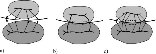
Figure 16. Comparison of generic bifurcation of the full Blum linking structure versus evolution of the retracted skeletal linking structure for two evolving regions $\Omega^{\prime}_{i\,t}$ becoming generically adjoined as in Figure 15. Full Blum linking structure bifurcates by adding branches from a) unjoined regions to b) after becoming adjoined. By contrast, the retracted skeletal linking structure evolves while retaining the structure of the skeletal sets, from a) unjoined regions to c) after being adjoined.

Retracting Full Blum Linking Structure via Smoothing

We consider a second situation where we modify the full Blum linking structure of a configuration with adjoining regions to a skeletal linking structure. We do this using a “smoothing of the corners of the regions”, in a small neighborhood of the singular set. To precisely describe this we suppose we have a multi-region configuration $\boldsymbol{\Omega}$, which includes regions which adjoin, modeled by $\Phi:\boldsymbol{\Delta}\to{\mathbb{R}}^{n+1}$, so that it exhibits a generic full Blum medial structure, with $(M_{i},U_{i},\ell_{i})$ the Blum medial structure for each $\Omega_{i}$, and $M_{0}$ the external medial linking axis. Given a neighborhood $W$ of the singular set of $\boldsymbol{\Omega}$, i.e. the union of the singular strata of the boundaries, the goal is to modify the regions $\Omega_{i}$ in the neighborhood $W$ so that the region boundaries are smooth and agree with the original boundaries outside of $W$, and such that the resulting Blum medial axes extend to a skeletal structure for $\boldsymbol{\Omega}$.

Definition 5.1.

A smoothing of the configuration $\boldsymbol{\Omega}$ defined by $\Phi$, with a neighborhood $W$ of the singular set of $\boldsymbol{\Omega}$, consists of a disjoint configuration $\boldsymbol{\Delta}^{\prime}$, with a region $\Delta^{\prime}_{i}$ for each $\Delta_{i}$, and an embedding $\Phi^{\prime}:\boldsymbol{\Delta}^{\prime}\to{\mathbb{R}}^{n+1}$ satisfying the following conditions. We let $\Omega_{i}^{\prime}=\Phi^{\prime}(\Delta^{\prime}_{i})$ and $\mathcal{B}_{i}^{\prime}=\Phi^{\prime}(X^{\prime}_{i})$. There is a neighborhood $W^{\prime}\subset W$ such that:

• Each $\Omega_{i}^{\prime}\subset\Omega_{i}$, and $\Omega_{i}^{\prime}$ has a generic Blum medial axis $M_{i}^{\prime}$ such that $\mathcal{B}_{i}^{\prime}\backslash W^{\prime}=\mathcal{B}_{i}\backslash W^{\prime}$. Moreover, the portion of the medial axis of $\Omega_{i}$ defined from $W^{\prime}\cap\mathcal{B}_{i}$ is contained in $W$ so that $M_{i}^{\prime}=M_{i}$ off $W$.

• The radial flow of $\Omega_{i}^{\prime}$ from $M_{i}^{\prime}\cap W$ is nonsingular and remains transverse to the radial lines out to and including its first intersection with $M_{0},$ and the radial lines intersect both $\mathcal{B}_{i}$ and $M_{0}$ transversally (including the limiting tangent spaces of it at singular points). This agrees with the radial flow for the full Blum structure off $W^{\prime}$.

• The pull-back of the singular set of $M_{0}$ by the radial flow in ii) refines the stratification of $\tilde{M}_{i}^{\prime}$ on $W^{\prime}$.

Remark 5.2.

The verification that the radial flow is nonsingular and transverse to the radial lines is done using the radial and edge curvature conditions in [D1, Thm. 2.5]

An example of such a smoothing is given in Figure 17.

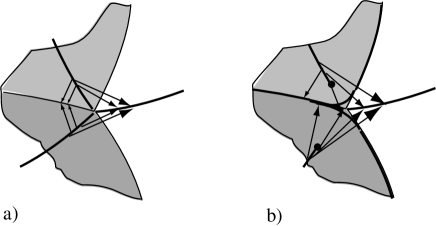
Figure 17. An example of a smoothing of a configuration with adjoining regions $\Omega_{1}$ and $\Omega_{2}$ in the neighborhood of a corner point with linking vector fields shown: a) Blum linking structure and b) Smoothing and resulting retracted skeletal linking structure.

The smoothing gives rise to a skeletal linking structure as follows.

Proposition 5.3.

For a configuration of regions with generic full Blum linking structure, a smoothing of the configuration allows the Blum linking structure to be replaced by a skeletal linking structure.

Proof.

To define the skeletal structure, given the smoothing, we begin by letting the skeletal set in each $\Omega_{i}$ be the Blum medial axis $M_{i}^{\prime}$ for $\Omega_{i}^{\prime}$. By ii) the radial lines from $M_{i}^{\prime}$ extend to the boundary $\mathcal{B}_{i}$ and the vectors from points $x\in M_{i}^{\prime}$ to the intersection points of the radial lines from $x$ with $\mathcal{B}_{i}$ are the radial vectors $U_{i}^{\prime}$ for the skeletal structure. The stratification of $\tilde{M}_{i}^{\prime}$ is given by the refinement $\tilde{M}_{i}^{\prime\prime}$ of $\tilde{M}_{i}^{\prime}$ given by condition iii). Since the singular set of each $\mathcal{B}_{i}$ is a portion of the singular set of $M_{0}$, condition iii) guarantees that the radial flow is nonsingular and smooth on the strata out to the boundary $\mathcal{B}_{i}$.

To extend the individual skeletal structures on the $\Omega_{i}$ to a skeletal linking structure, we use $M_{0}$ for the external linking medial axis. We use the extensions of the radial lines of $\Omega_{i}^{\prime}$ until they meet $M_{0}$. These extensions define the linking vector fields $L_{i}$, which agree with the Blum linking vector fields off $W^{\prime}$. The linking flow will agree with that for the Blum structure off $W^{\prime}$. On $M_{i}^{\prime}\cap W^{\prime}$ the linking flow will agree with the radial flow in $\mathcal{B}_{i}$. From $\mathcal{B}_{i}$ to $M_{0}$, the radial flow will be nonsingular and transverse to the radial lines. It follows by the radial, edge, and linking curvature conditions (see Propositions 7.4 and 8.1 in §§7 and 8), that the linking flow is also nonsingular and transverse to the radial lines. Lastly, since both the radial flow and linking flow have the radial lines as flow lines, the inverse image of the singular set of $M_{0}$ under the linking flow will be the same as for the extended radial flow. By the definition of the refinement of $\tilde{M}_{i}^{\prime}$ in iii), the $L_{i}^{\prime}$ (and hence $\ell_{i}^{\prime}=\|L_{i}^{\prime}\|$) will be smooth on the strata of the refinement.

Thus, the collection of $(M_{i}^{\prime},U_{i}^{\prime},\ell_{i}^{\prime})$ define the resulting skeletal linking structure. ∎

We indicate an approach to constructing a smoothing of the corners of a configuration. However, we will not give the details here to verify that the conditions are satisfied. First, we construct for each region $\Omega_{i}$ a smooth function $f_{i}$ defined on a neighborhood of $\Omega_{i}$ such that: $f_{i}\geq 0$ on $\Omega_{i}$, $f_{i}\equiv 0$ on $\mathcal{B}_{i}$, with ${\rm grad}\,(f_{i})$ non zero on the smooth points of $\mathcal{B}_{i}$; and second, in a neighborhood of a $k$-edge-corner point the normal lines to the level sets of $f_{i}$ meet the limiting tangent planes of both the boundary and the external medial axis transversally. Next, we use a bump function $\delta_{i}$ which does not vanish on ${\rm sing}\,(\mathcal{B}_{i})$ and has its support in a neighborhood $W$ of ${\rm sing}\,(\mathcal{B}_{i})$, and so that it and its first derivatives (in the corner coordinates) are bounded by $\varepsilon>0$. Then, the hypersurface defined by $f_{i}(x)=\delta_{i}(x)$ will satisfy the conditions for a sufficiently small $W$ and appropriate $\delta_{i}$. To construct $f_{i}$ we use the local model coordinates for a $k$-edge-corner point. We then use a partition of unity to piece together functions of the form $h=g\cdot\prod_{j=1}^{k}x_{j}$, with ${\rm grad}\,(g)$ pointing into $\Omega_{i}$ and $g$ nonvanishing on the boundary. This gives the desired smoothing.

6. Questions Involving Positional Geometry of a Multi-region Configuration

Introduction

Having introduced medial/skeletal linking structures for a multiregion configuration $\boldsymbol{\Omega}=\{\Omega_{i}\}$ in ${\mathbb{R}}^{n+1}$ in Part I, we now develop an approach to the “positional geometry”  of the configuration using mathematical tools defined in terms of the linking structure. We do so by building upon the methods already developed in the case of a single region with smooth boundary [D1], [D2]. Moreover, we will see that certain constructions and operators used for determining the geometry of single regions can be combined to give geometric properties of the configuration.

There are several possible aspects to this. One approach is to measure the differences between two configurations. More generally given a collection of configurations, we may ask what are the statistically meaningful shared geometric properties of the collection of configurations, and how do the geometric properties of a particular configuration differ from those for the collection. To provide quantitative measures for these properties, we will directly associate geometric invariants to a configuration. Such invariants may be globally defined depending on the entire configuration or locally defined invariants depending on local subconfigurations associated to each region.

For example, if we view the union of the regions as a topological space, then we can measure the Gromov-Hausdorff distance between two such configurations. We may also use the geodesic distance between the two configurations measured in a group of global diffeomorphisms mapping one configuration to another. Such invariants give a single numerical global measure of differences between two configurations. Instead, we will use skeletal linking structures associated to the configurations to directly associate both global and local geometric invariants which can be used to measure the differences between a number of different features of configurations.

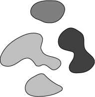
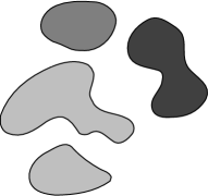
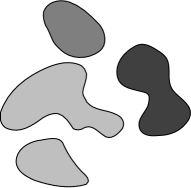
(a)                                   (b)                                   (c)

Figure 18. Images exhibiting configurations of four regions. A basic problem is to determine the differences between the configurations that are due to changes in shapes of the regions versus those due to changes in positions. Furthermore, one would want to find invariants which capture these differences.

In introducing these invariants, we will be guided by several key considerations. The first involves distinguishing between the differences in the shapes of individual regions versus their positional differences and how each of these contributes to the differences in the configurations. As illustrated in Figure 18, the three configurations differ; but it is not clear to what extent this is due to shape differences of the regions versus changes in position, nor how these different contributions should be measured.

In measuring the relative positions of the regions, more than just the minimum distance between region boundaries is required. As illustated in Figure 19, while region $\Omega_{3}$ touches $\Omega_{1}$, it does so only on a small portion of $\Omega_{3}$. By comparison, $\Omega_{2}$ does not touch $\Omega_{1}$, but it remains close over a larger region. A goal is to define a numerical measure of closeness of regions which takes into account both aspects. Related to this is the issue of which regions that do not touch should be considered neighbors and what should be the criterion?

Figure 19. Measuring closeness of regions in a configuration. Although $\Omega_{3}$ touches $\Omega_{1}$, only a small portion of $\Omega_{3}$ is close to $\Omega_{1}$. In contrast, $\Omega_{2}$ does not touch $\Omega_{1}$, but it remains close over a larger region.

A third issue for a configuration is viewing it as a hierarchy of the regions, indicating which regions are most central to the configuration and which are less geometrically significant. For example in Figure 20, the position of region $\Omega_{1}$ makes it more important for the overall configuration in b) than in a), where it is more of an “outlier”. For example, a small movement of $\Omega_{1}$ in a) would be less noticeable and have a smaller effect to the overall configuration than in b). By having a smaller effect we mean that the deformed configuration could be mapped to the original by a diffeomorphism which has smaller local distortions near the configuration in the case of a) versus b). We will also provide a numerical measure of geometric significance of a region for the configuration.

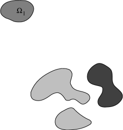
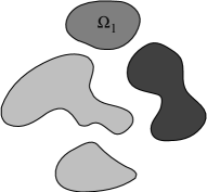
(a)                                   (b)

Figure 20. Images exhibiting configurations of four regions. In a), region $\Omega_{1}$ is a greater distance from the remaining regions, and hence is less significant when modeling the configuration. In b), the closeness of region $\Omega_{1}$ to the other regions makes it more significant for the configuration.

Along with issues of closeness, significance and hierarchy, there is also the question of when there are natural subconfigurations. An example of this is seen in Figure 21. In a) is shown a configuration with distinct subconfigurations. As these subconfigurations are moved together, a point is reached when they are no longer distinguished by geometric features. This raises the question of whether there are numerical invariants which can be used to determine when there are identifiable subconfigurations.

We will combine the invariants which measure these geometric features to provide a “tiered graph structure”, which is a graph with vertices representing the regions, edges between vertices of neighboring regions, and values of significance assigned to the vertices, and closeness assigned to the edges. Then, as thresholds for closeness and significance vary, the resulting subgraph satisfying the conditions will exhibit the central regions of the configuration, various subgroupings of regions and the hierarchy of relations between the regions.

Our goal in the subsequent sections is to first use the skeletal linking structure to identify neighboring regions and introduce linking neighborhoods between the regions. Second, we will introduce numerical “volumetric invariants”  for the indicated measures. In turn, we will use the skeletal linking structure to compute the volumetric invariants via “skeletal linking integrals”computed on the skeletal sets.

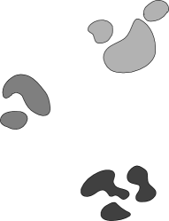
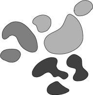
(a)                                   (b)

Figure 21. Subconfigurations of regions. In a) a configuration is formed from three groups of regions. In b), the groups of regions have been moved closer; based on geometric position, the groups are no longer clearly distinguished.

7. Shape Operators and Radial Flow for a Skeletal Structure

In preparation for obtaining the desired properties of the linking flow, we recall how for the skeletal structure $(M,U)$ for a single region $\Omega$ we may introduce radial and edge shape operators. Using them, we have sufficient conditions for the nonsingularity of the radial flow and smoothness of the associated boundary (see [D1]). Furthermore, these operators can be used to compute both the intrinsic differential geometry of the boundary and the global geometry of the region (using “skeletal integrals”  on $\tilde{M}$, see e.g. [D2] and [D4]). Our eventual goal is to show using the skeletal linking structure that these results can be extended to the entire multi-region configuration.

The Radial Flow

In §3, we briefly recalled how from a skeletal structure $(M,U)$ in ${\mathbb{R}}^{n+1}$, we can define the “associated boundary”

$$\mathcal{B}\,\,=\,\,\{x+U(x):x\in M,\,\mbox{ all values of }U\}\,.$$

However, conditions are required on the skeletal structure to ensure that the boundary is smooth. This is achieved using the radial flow and the radial map which is the time one map of the radial flow. This allows us to establish additional properties of the region $\Omega$ bounded by $\mathcal{B}$. The radial flow is defined as a map from the “normal line bundle”  $N$ on $\tilde{M}$, the “double of $M$”  which has a finite-to-one stratified mapping $\pi:\tilde{M}\to M$. In the neighborhood $W$ of a point $x_{0}\in M$ with a smooth single-valued choice for $U$, we define a local representation of the radial flow by $\psi_{t}(x)=x+t\cdot U(x)$, $1\leq t\leq 1$, and the radial map $\psi_{1}(x)=x+U(x)$. Together the local $\psi_{t}$ define a global map $\psi:N\to{\mathbb{R}}^{n+1}$. We will next recall the role of the radial and edge shape operators in guaranteeing the nonsingularity of the radial flow and the smoothness of the level sets $\mathcal{B}_{t}=\{x+t\cdot U(x):x\in M,\,\mbox{ all values of }U\}$.

Radial and Edge Shape Operators

We define “shape operators”for the skeletal structure $(M,U)$. At a smooth point $x_{0}$ of $M$ we choose a “smooth value”of $U$. We recall from §3 that in a neighborhood of any smooth point of $M$ (i.e. a point in $M_{reg}$), values of $U$ on one side form a smooth vector field. By a smooth value of $U$ we mean such a smooth choice of $U$ values. Then, $U=r\cdot\mathbf{u}$ for a unit radial vector field $\mathbf{u}$.

Radial Shape Operator: We define for $v\in T_{x_{0}}M$

$$S_{rad}(v)\quad=\quad-{\rm proj}_{U}(\dfrac{\partial\mathbf{u}}{\partial v})$$

where ${\rm proj}_{U}$ denotes projection onto $T_{x_{0}}M$ along $U$ (in general, this is not orthogonal projection, see a) in Figure 22). The principal radial curvatures $\kappa_{r\,i}$ are the eigenvalues of $S_{rad}$. For a basis $\mathbf{v}=\{v_{1},\dots,v_{n}\}$ for $T_{x_{0}}M$, we let $S_{\mathbf{v}}$ denote the matrix representation of $S_{rad}$ with respect to $\mathbf{v}$.

For a non–edge point $x_{0}\in M$, a value of $U$ extends to be smooth on some local neighborhood of $x_{0}$ on any regular stratum containing $x_{0}$ in its closure. For this smooth value of $U$, we may likewise define the radial shape operator at $x_{0}$. Thus, the radial shape operator is also multivalued in that at a non–edge point $x_{0}$ there will be a radial shape operator for each value of $U$ at $x_{0}$, which at smooth points of $M$ means a value for each side of $M$.

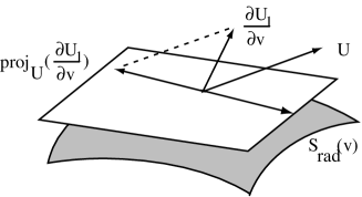
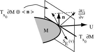
a)                                                         b)

Figure 22. Illustrated in a) is the radial shape operator and in (b) the edge shape operator.

Edge Shape Operator: For an edge (closure) point $x_{0}$, a smooth value of $U$ is a smoothly varying choice of values for $U$, defined on a neighborhood of $x_{0}$ one side of $M$ for edge coordinates. Then for a normal vector field $\mathbf{n}$ to $M$ on the same side of $M$ as $U$, we define

$$S_{E}(v)\quad=\quad-{\rm proj}^{\prime}(\dfrac{\partial\mathbf{u}}{\partial v})\,.$$

Here ${\rm proj}^{\prime}$ denotes projection onto $T_{x_{0}}\partial M\oplus<\mathbf{n}>$ along $U$ (again this is not orthogonal, see b) in Figure 22). Let $\mathbf{v}=\{v_{1},\dots,v_{n}\}$ be a basis of $T_{x_{0}}M$ so that $\{v_{1},\dots,v_{n-1}\}$ is a basis $T_{x_{0}}\partial M$, and $v_{n}$ maps under the edge parametrization map to $c\cdot U$ for $c\geq 0$. We refer to $\mathbf{v}$ as a special basis for $T_{x_{0}}M$. Then, $S_{E\,\mathbf{v}}$ is a matrix representation of $S_{E}$ with respect to the basis $\mathbf{v}$ in the source and $\{v_{1},\dots,v_{n-1},\mathbf{n}\}$ in the target. We let $I_{n-1,1}$ be the $n\times n$–diagonal matrix with $1$’s in the first $n-1$ diagonal positions and $0$ in the last. The principal edge curvatures $\kappa_{E\,i}$ are the generalized eigenvalues of $(S_{E\,\mathbf{v}},I_{n-1,1})$ (i.e. $\lambda$ such that $S_{E\,\mathbf{v}}-\lambda\cdot I_{n-1,1}$ is singular).

Curvature Conditions and Nonsingularity of the Radial Flow

We now recall conditions guaranteeing the smoothness of the radial flow on smooth strata and the resulting smoothness of the level sets. We emphasize that this is a local result as neither the flow defined on a stratified set nor its level sets are smooth, but rather they are stratified. Along with the radial and edge shape operators, an important role is also played by the multi-valued compatibility $1$-form $\eta_{U}=dr+\omega_{U}$, where $\|U\|=r$ is the radial function and $\omega_{U}(v)=v\cdot\mathbf{u}$ for $U=r\cdot\mathbf{u}$, with $\mathbf{u}$ the multivalued unit vector field along $U$. Then, $\eta_{U}$ is also multivalued with one value for each value of $U$.

Then, we consider the following three conditions for a skeletal structure $(M,U)$:

1. (Radial Curvature Condition ) for a point $x_{0}\in M\backslash\partial M$ and all values $U(x_{0})$

   $$r<\min\{\frac{1}{\kappa_{r\,i}}\}\quad\mbox{ for all positive principal radial curvatures }\kappa_{r\,i}\,;$$

2. (Edge Condition ) for a point $x_{0}\in\overline{\partial M}$ (closure of $\partial M$) ;

   $$r<\min\{\frac{1}{\kappa_{E\,i}}\}\quad\mbox{ for all positive principal edge curvatures }\kappa_{E\,i}$$

3. (Compatibility Condition ) for a point $x_{0}\in M$ (which includes edge points), $\eta_{U}\equiv 0$.

Remark 7.1.

The radial curvature, edge, and compatibility conditions involve choices of values for $U$ and hence are multi-valued conditions at each point. In the radial curvature condition it is to be understood that the $r$ value associated to a given value of $U$ satisfies the inequality for the shape operator associated to that value. Thus, at smooth points of $M$, we have inequalities corresponding to each side of $M$.

The first two conditions allow us to control the local behavior of the radial flow, ensuring that singularities do not develop from smooth points, nor further singularities from singular or edge points.

While the first two conditions are open conditions and hence robust, the third compatibility condition is not and reveals an essential feature about the level sets of the flow. For any time $t<1$ the level sets are singular at points coming from the singular points of $M$ (including edge points). The compatibility condition at singular points of $M$ ensures that only at $t=1$ when the flow reaches the boundary do the singularities simultaneously disappear so the boundary becomes weakly $C^{1}$ at the points corresponding to singular points of $M$ (which means there are unique limiting tangent spaces at these points, and as a consequence the boundary is $C^{1}$ at points coming from the strata of codimension $1$, see [D1, Lemma 5.4]). However, if the compatibility condition does not hold on a stratum, then the boundary may have edges and corners at these image points. Hence, skeletal structures can also be used for regions with boundaries and corners.

Local Nonsingularity of the Flow from Smooth and Edge Points

We begin by stating how the radial curvature and edge conditions imply the local nonsingularity of $\psi$ and $\psi_{t}$ (these are given in [D1, Props. 4.1 and 4.4]).

Proposition 7.2.

Let $U$ be a smooth value of the radial vector field defined in a neighborhood $W$ of $x_{0}\in M$. Suppose either that $x_{0}\in M_{reg}$ and satisfies the radial curvature condition in the neighborhood $W$; or $x_{0}\in\partial M$ (or is an edge closure point) and satisfies the edge condition on the neighborhood $W$. Then,

1. $\psi:W\times{\mathbb{R}}\to{\mathbb{R}}^{n+1}$ is a local diffeomorphism at $(x_{0},t)$ for $0<t\leq 1$ (and also $t=0$ for smooth points);

2. $\psi_{t}:W\to{\mathbb{R}}^{n+1}$ is a local embedding at $x_{0}$ for any $0\leq t\leq 1$; and

3. $\psi_{t}(W)$ is transverse to the line spanned by $U$ for each $0\leq t\leq 1$.

   Conversely, suppose $\psi$ is nonsingular at $(x_{0},t)$ for $0<t\leq 1$, which is equivalent to $\psi_{t}(W)$ being nonsingular at $\psi_{t}(x_{0})$ and transverse to the radial line for $0<t\leq 1$. Then the radial, resp. edge, curvature condition is satisfied for $x_{0}$ and the value $U$, depending on whether $x_{0}$ is a nonedge closure point, resp. an edge closure point.

Although only one direction for this proposition was proven in the propositions just cited in [D1], an examination of the proof given there also establishes the converse. $\Box$

Global Nonsingularity of the Radial Flow

The preceding local results at all points of $M$ can be combined with the compatibility condition at singular points to yield the following global result (given in [D1, Thm. 2.5]).

Theorem 7.3.

Let $(M,U)$ be a skeletal structure which satisfies: the radial curvature condition at all nonedge points, the edge condition at edge points and edge closure points, and the compatibility condition at all singular points. Then (see Figure 23):

1. The associated boundary $\mathcal{B}$ is an immersed topological manifold which is smooth at all points except those corresponding to points of $M_{sing}$.

2. At points corresponding to points of $M_{sing}$, it is weakly $C^{1}$ (this implies that it is $C^{1}$ on the points which are in the images of strata of codimension $1$).

3. At smooth points, the projection along the lines of $U$ will locally map $\mathcal{B}$ diffeomorphically onto the smooth part of $M$.

4. Also, if there are no nonlocal intersections, then $\mathcal{B}$ will be an embedded manifold and $\Omega\backslash M$ is fibered by the level sets $\mathcal{B}_{t}$, $0<t\leq 1$.

Figure 23. Illustrating the radial flow from the skeletal set $M$, with the radial vector field $U$, flowing in the region $\Omega$ to the boundary $\mathcal{B}$, where the level sets are stratified sets forming a fibration of $\Omega\backslash M$.

This allows us to completely describe the structure of the interior of the regions in a multi-region configuration. This extends to the geometry via the next results.

Evolution of the Shape Operators under the Radial Flow

The last feature of the radial flow which we recall is the evolution of the radial and edge shape operators under the radial flow, with the eventual goal of extending these results to the linking flow. This allows us to relate in the Blum case the radial geometry on the medial axis with the differential geometry of the boundary.

We first consider the evolution of the radial shape operator under the radial flow. Let $x_{0}\in M_{reg}$, and let $\{v_{1},\dots,v_{n}\}$ be a basis for $T_{x_{0}}M$. We suppose we have chosen a smooth value of $U$ in a neighborhood of $x_{0}$. If $x_{0}$ is a non–edge singular point, then we can carry out an analogous argument on a local component for $x_{0}$.

For a given $t$, let

$$v_{i}^{\prime}=d\psi_{t}(v_{i})=\dfrac{\partial\psi_{t}}{\partial v_{i}}\quad\mbox{for }i=1,\dots,n.$$

With $r$ denoting the radial function as in §3, we suppose that $\frac{1}{tr}$ is not an eigenvalue of $S_{rad}$ (at $x_{0}$). Then, by the proof of Proposition 4.1 of [D1], $\psi_{t}$ maps a neighborhood $W$ of $x_{0}$ diffeomorphically to a smooth submanifold transverse to $U(x_{0})$. Thus, the image of $U$ along $\psi_{t}$ remains transverse in some neighborhood of $x_{0}^{\prime}=\psi_{t}(x_{0})$ to $W^{\prime}=\psi_{t}(W)\subset\mathcal{B}_{t}$. Hence, it has a well-defined radial shape operator, which we denote by $S_{rad\,t}$. We will compute $S_{\mathbf{v}^{\prime}\,t}$, the matrix representation of $S_{rad\,t}$ with respect to the basis $\{v_{i}^{\prime}\}$.

Then, the following two results are consequences of Proposition 2.1 and Corollary 2.2 of [D2].

Evolution of the Radial Shape Operator from Smooth Points

Proposition 7.4.

Suppose that at a smooth point $x_{0}\in M_{reg}$, we have a smooth value of $U$ and a basis $\{v_{i}\}$ for $T_{x_{0}}M$. Let $\{v_{i}^{\prime}\}$ denote the image of $\{v_{i}\}$ under $d\psi_{t}(x_{0})$. If $\frac{1}{tr}$ is not an eigenvalue of the radial shape operator $S_{\mathbf{v}}$ at $x_{0}$, then the radial shape operator $S_{\mathbf{v}^{\prime}\,t}$ for $\mathcal{B}_{t}$ at $x_{0}^{\prime}=\psi_{t}(x_{0})$ for the corresponding smooth value of $U$ is given by

(7.1) $$S_{\mathbf{v}^{\prime}\,t}\quad=\quad(I-tr\cdot S_{\mathbf{v}})^{-1}S_{\mathbf{v}}\,.$$

With the identification of the tangent spaces $d\psi_{t}(x):T_{x}M\simeq T_{\psi_{t}(x)}\mathcal{B}$, we may write the preceding in the basis independent form

(7.2) $$S_{rad,t}\,\,=\,\,(I-tr\cdot S_{rad})^{-1}S_{rad}\,.$$

Remark 7.5.

If the compatibility $1$-form $\eta_{U}$ vanishes on an open subset of $\tilde{M}_{reg}$, then $U$ will be orthogonal to $\mathcal{B}$ at each point of its the image under the radial flow (see §7) as happens for the Blum case. It follows that the formula (7.1) gives the differential geometric shape operator for $\mathcal{B}$; thus, capturing the geometry of the boundary, see [D2].

Principal Radial Curvatures for $\mathcal{B}_{t}$

Then, we can deduce information about the principal radial curvatures at $x_{0}^{\prime}$ in terms of those at $x_{0}$.

Corollary 7.6.

Under the assumptions of Proposition 7.4, there is a correspondence (counting multiplicities) between the principal radial curvatures $\kappa_{r\,i}$ of $M$ at $x_{0}$ and $\kappa_{r\,t\,i}$ of $\mathcal{B}_{t}$ at $x_{0}^{\prime}$ given by

$$\kappa_{r\,t\,i}=\frac{\kappa_{r\,i}}{(1-tr\kappa_{r\,i})}\quad\mbox{or equivalently}\quad\kappa_{r\,i}=\frac{\kappa_{r\,t\,i}}{(1+tr\kappa_{r\,t\,i})}\,.$$

Furthermore, if $e_{i}$ is an eigenvector for the eigenvalue $\kappa_{r\,i}$ of $S_{rad}$, then $e_{i}^{\prime}$, which has the same coordinates with respect to $\mathbf{v}^{\prime}$ as $e_{i}$ has with respect to $\mathbf{v}$, is an eigenvector with eigenvalue $\kappa_{r\,t\,i}$ of $S_{rad,t}$.

Evolution of the Radial Shape Operator from Edge Points

We can carry out an analogous line of reasoning for the evolution of the radial shape operator for points corresponding to an edge point $x_{0}$. A smooth value of $U$ in a neighborhood of $x_{0}$ corresponds to one side of $M$. Although $\mathcal{B}_{t}$ is not smooth at $\psi_{t}(x_{0})$ if $t<1$, we note that by Proposition 4.4 of [D1], provided $\frac{1}{tr}$ is not a generalized eigenvalue for $(S_{E\,\mathbf{v}},I_{n-1,1})$, the one side of $\mathcal{B}_{t}$ corresponding to $U$ is smooth and is transverse to $U$ at $x_{0}$ when $t>0$. Thus, the radial shape operator is defined for $\mathcal{B}_{t}$ at points corresponding to edge points when $t>0$. Hence, we may compute the radial shape operator $S_{\mathbf{v}^{\prime}t}$ for this one side using [D2, Proposition 2.3] as follows.

Proposition 7.7.

Suppose that at an edge point $x_{0}\in\overline{\partial M}$, we have a smooth value of $U$ (corresponding to one side of $M$) and a special basis $\{v_{i}\}$ for $T_{x_{0}}M$. Let $\{v_{i}^{\prime}\}$ denote the image of $\{v_{i}\}$ under $d\psi_{t}(x_{0})$. If $\frac{1}{tr}$ is not a generalized eigenvalue of $(S_{E\,\mathbf{v}},I_{n-1,1})$, then the radial shape operator $S_{\mathbf{v}^{\prime}\,t}$ for $\mathcal{B}_{t}$ at $x_{0}^{\prime}=\psi_{t}(x_{0})$ is given by

(7.3) $$S_{\mathbf{v}^{\prime}\,t}\quad=\quad(I_{n-1,1}-tr\cdot S_{E\,\mathbf{v}})^{-1}S_{E\,\mathbf{v}}\,.$$

We note that unlike the situation for the radial shape operator, $S_{E\,\mathbf{v}}$ does not necessarily commute with $I_{n-1,1}$ so the order of the factors is important.

Unlike the case of non–edge points, we cannot in general deduce a simple formula for the principal radial curvatures for $S_{\mathbf{v}^{\prime}\,t}$ in terms of the principal edge curvatures. However, in certain special cases, we can carry out the calculations (see e.g. [D2] or [D7]).

8. Linking Flow and Curvature Conditions

We consider a skeletal linking structure $\{(M_{i},U_{i},\ell_{i})\}$. If each $(M_{i},U_{i},)$ satisfies the conditions of Theorem 7.3, then we obtain regions $\Omega_{i}$ which, provided the regions are disjoint or intersect appropriately, give a multi-region configuration $\boldsymbol{\Omega}=\{\Omega_{i}\}$. There are additional conditions to be satisfied for $\{(M_{i},U_{i},\ell_{i})\}$ to be the skeletal linking structure for $\boldsymbol{\Omega}$. One part of this requires properties of the linking flow. Using analogs of the preceding results for the radial flow, we will give sufficient conditions for nonsingularity of the linking flow. We also will derive analogous formulas for the evolution of the radial and edge shape operators under the linking flow.

Nonsingularity of the Linking Flow

We first establish the conditions for the nonsingularity of the linking flow $\lambda$ (or $\lambda_{t}$) introduced in the definition of the skeletal linking structure (see (3.1) in §3). For the skeletal linking structure $\{(M_{i},U_{i},\ell_{i})\}$, we have the following two conditions:

1. (Linking Curvature Condition ) For all points $x_{0}\in M_{i}\backslash\partial M_{i}$ and all values $U_{i}(x_{0})$,

   $$\ell_{i}<\min\{\frac{1}{\kappa_{r\,j}}\}\quad\mbox{ for all positive principal radial curvatures }\kappa_{r\,j}\,;$$

2. (Linking Edge Condition ) For all points $x_{0}\in\overline{\partial M_{i}}$ (the closure of $\partial M_{i}$)

   $$\ell_{i}<\min\{\frac{1}{\kappa_{E\,j}}\}\quad\mbox{ for all positive principal edge curvatures }\kappa_{E\,j}\,.$$

Then, given a skeletal structure $\{(M_{i},U_{i},\ell_{i})\}$ the smoothness of the linking flow is guaranteed by the following analog of Proposition 7.2.

Proposition 8.1.

Let $U$ be a smooth value of the radial vector field defined in a neighborhood $W$ of $x_{0}\in M_{i}$. Suppose either that $x_{0}\in M_{i}\backslash\partial M_{i}$ and satisfies the linking curvature condition in the neighborhood $W$; or $x_{0}\in\overline{\partial M_{i}}$ and satisfies the linking edge condition on the neighborhood $W$. Then,

1. $\lambda:W\times{\mathbb{R}}\to{\mathbb{R}}^{n+1}$ is a local diffeomorphism at $(x_{0},t)$ for $0<t\leq 1$ (and also $t=0$ for nonedge closure points);

2. $\lambda_{t}:W\to{\mathbb{R}}^{n+1}$ is a local embedding at $x_{0}$ for any $0\leq t\leq 1$; and

3. $\lambda_{t}(W)$ is transverse to the line spanned by $U$ for each $0\leq t\leq 1$.

   Conversely, suppose $\lambda$ is nonsingular at $(x_{0},t)$ for $0<t\leq 1$, which is equivalent to $\lambda_{t}(W)$ being nonsingular at $\lambda_{t}(x_{0})$ and transverse to the line spanned by $U$ for $0<t\leq 1$. Then the linking curvature, resp. linking edge condition is satisfied at $x_{0}$, depending on whether it is a nonedge closure point, resp. an edge closure point.

Then, we can combine these conditions to conclude the following.

Corollary 8.2.

For a skeletal structure $\{(M_{i},U_{i},\ell_{i})\}$, if the linking curvature condition or linking edge condition is satisfied at all points of a stratum $S_{j}$ of $\tilde{M}_{i}$, then the linking flow from $S_{j}$ is nonsingular and remains transverse to the radial lines.

Thus, the images of strata of the labelled refinement of each $\tilde{M}_{i}$ under the linking flow are immersed submanifolds for all $0<t\leq 1$, and provided distant points from the same strata are not linked, then the images of strata are submanifolds.

Proof of Proposition 8.1.

First, we may view the linking flow from $M_{i}$ for $t>\frac{1}{2}$ as the composition of the flow for $t=\frac{1}{2}$, with level set the boundary $\mathcal{B}_{i}$, followed by a flow from $\mathcal{B}_{i}$ for time $t^{\prime}=2(t-\frac{1}{2})$. Thus, for $\frac{1}{2}\leq t\leq 1$, if we denote the radial flow by $\psi_{t}$, then $\lambda_{t}(x)=\psi_{1}(x)+(\chi(t)-r_{i}(x))\mathbf{u}_{i}(x)$ (with $\chi(t)$ as defined in (3.1)). Hence, the linking flow can itself be viewed as a radial flow for $(\mathcal{B}_{i},U_{i}^{\prime})$ at the point $x_{0}^{\prime}=\lambda_{\frac{1}{2}}(x_{0})$ reparametrized at twice the speed. Here the vector field $U_{i}^{\prime}$ is the translate along the radial lines to $x_{0}^{\prime}$ of the vector field $(\ell_{i}-r_{i})\mathbf{u}_{i}$, where $\mathbf{u}_{i}$ is the unit vector field in the direction of $U_{i}$.

As $r_{i}\leq\ell_{i}$, the linking radial curvature and linking edge conditions imply the corresponding radial curvature and edge conditions for the radial flow. Hence, by Proposition 7.2 we have nonsingularity of the linking flow and the level surfaces for $0<t\leq\frac{1}{2}$, with the level surfaces transverse to the radial lines. Also, at $t=\frac{1}{2}$, the level surface is the boundary $\mathcal{B}_{i}$ of the associated region $\Omega_{i}$.

Then, we can further verify the nonsingularity of the linking flow for $\frac{1}{2}<t\leq 1$, and the corresponding level sets by again applying the radial curvature conditions to $(\mathcal{B}_{i},U_{i}^{\prime})$ .

Now, $t^{\prime}=2(t-\frac{1}{2})$, and

$$\chi(t)-r_{i}\,\,=\,\,2(t-\textstyle{\frac{1}{2}}\displaystyle)(\ell_{i}-r_{i})\,\,=\,\,t^{\prime}(\ell_{i}-r_{i}).$$

Thus, the linking flow for $\frac{1}{2}\leq t\leq 1$ gives the radial flow for $(\mathcal{B}_{i},U_{i}^{\prime})$ for $0\leq t^{\prime}\leq 1$. Hence, by Proposition 7.7 we obtain

(8.1) $$S_{\mathbf{v}^{\prime\prime},t}\,\,=\,\,(I-(\chi(t)-r_{i})S_{\mathbf{v}^{\prime},\frac{1}{2}})^{-1}S_{\mathbf{v}^{\prime},\frac{1}{2}}\,,$$

where $S_{\mathbf{v}^{\prime},\frac{1}{2}}$ is the matrix representation for the radial shape operator for $(\mathcal{B}_{i},U_{i}^{\prime})$ at $x_{0}^{\prime}$ with respect to the basis $\mathbf{v}^{\prime}$ corresponding to the basis $\mathbf{v}$ for $T_{x_{0}}M$ under the radial flow.

However, by Proposition 7.2, the radial curvature condition is equivalent to the nonsingularity of $I-(\chi(t)-r_{i})S_{\mathbf{v}^{\prime},\frac{1}{2}}$ for $\frac{1}{2}<t\leq 1$; or equivalently the existence of $S_{\mathbf{v}^{\prime\prime},t}$ given by (8.1) for $\frac{1}{2}<t\leq 1$. We now claim there is an alternate formula for $S_{\mathbf{v}^{\prime\prime},t}$ given for $\frac{1}{2}<t\leq 1$ in the case of non-edge closure points $x_{0}$ by

(8.2) $$S_{\mathbf{v}^{\prime\prime},t}\,\,=\,\,(I-\chi(t)S_{\mathbf{v}})^{-1}S_{\mathbf{v}}\,,$$

where $S_{\mathbf{v}}$ is the matrix repesentation for the shape operator with respect to the basis $\mathbf{v}$. For edge closure points $x_{0}$, it is given by

(8.3) $$S_{\mathbf{v}^{\prime\prime},t}\,\,=\,\,(I_{n-1,1}-\chi(t)S_{E,\mathbf{v}})^{-1}S_{E,\mathbf{v}}\,,$$

with $S_{E,\mathbf{v}}$ denoting the matrix representation for the edge shape operator.

It then follows in the first case, that $S_{\mathbf{v}^{\prime\prime},t}$ will be defined for $0\leq t\leq 1$ provided $\frac{1}{\chi(t)}$ is not an eigenvalue for $S_{\mathbf{v}}$ for $0\leq t\leq 1$. This says that the eigenvalues of $S_{\mathbf{v}}$ do not lie in the interval $[\frac{1}{\ell_{i}},\infty)$, or that the positive eigenvalues of $S_{\mathbf{v}}<\frac{1}{\ell_{i}}$, which is equivalent to the linking curvature condition. Likewise, in the second case we require $\frac{1}{\chi(t)}$ is not a generalized eigenvalue for $(S_{E,\mathbf{v}},I_{n-1,1})$, for $0\leq t\leq 1$. Again, this is equivalent to the linking edge condition. This establishes the result. ∎

It remains to verify the assertions regarding (8.2) and (8.3). We do this by expressing the linking flow in either case via a semigroup of special Möbius tranformations on matrices and operators.

Special Möbius Transformations of Matrices and Operators

We will represent the evolved radial and edge shape operators under the linking flow as resulting from applying Möbius transformations to matrices and operators. We begin by considering for either $n\times n$ matrices $A$ and $B$ or operators $A,B:V\to V$, for $V$ a vector space of dimension $n$, a family of special Möbius transformations defined by

$$\Xi_{B,t}(A)\,\,=\,\,(B-tA)^{-1}A.$$

Here we view $B$ as fixed and either view $\Xi_{B,t}(A)$ as a function of $t\in{\mathbb{R}}$ for fixed $A$, or as a function of $A$ for fixed $t$. We observe that the evolution equations for both the radial and edge shape operators under the radial flow have this form for either $(A,B)=(S_{\mathbf{v}},I)$ or $(S_{E,\mathbf{v}},I_{n-1,1})$. We shall concentrate on the case of matrices, but the corresponding statements for operators are similar.

In general, if $\ker(A)\cap\ker(B)=0$, then $\Xi_{B,t}(A)$ is defined for all but the finite set of $t$ such that $\frac{1}{t}$ is not a generalized eigenvalue of $(A,B)$ (i.e. $\lambda$ so that $A-\lambda B$ is singular). Viewed as a function of $t$, we see

$$\dfrac{\partial(\Xi_{B,t}(A))}{\partial t}\,\, =\,\,-((B-tA)^{-1}(-A)(B-tA)^{-1})A$$

(8.4) $$=\,\,((B-tA)^{-1}A)^{2}=\,\,(\Xi_{B,t}(A))^{2}\,.$$

Thus, $\Xi_{B,t}(A)$ is a solution of the simplest matrix Riccati equation

(8.5) $$\dfrac{\partial\Xi_{B,t}(A)}{\partial t}\,\,=\,\,(\Xi_{B,t}(A))^{2}.$$

If $B$ is nonsingular, $\Xi_{B,t}(A)$ is the solution to the basic matrix Riccati equation (8.5) with initial condition $\Xi_{B,0}(A)=B^{-1}A$.

We consider the special cases of $\Xi_{B,t}(A)$ relevant for the evolution equations

$$\mu_{t}(A)\,\, =\,\,(I-tA)^{-1}A\qquad\text{ and }$$

(8.6) $$\nu_{t}(A)\,\, =\,\,(I_{n-1,1}-tA)^{-1}A\,.$$

For these to be well-defined we require for $\mu_{t}$ that $\frac{1}{t}$ is not an eigenvalue of $A$; while for $\nu_{t}$, we require that $\frac{1}{t}$ is not a generalized eigenvalue of $(A,I_{n-1,1})$.

If $B$ is nonsingular, then there is the relation

(8.7) $$\Xi_{B,t}(A)\,\,=\,\,((I-tB^{-1}A)^{-1}(B^{-1}A)\,,$$

so that

$$\Xi_{B,t}(A)\,\,=\,\,\mu_{t}(B^{-1}A)\,.$$

In particular, $\mu_{t}(A)$ is the basic solution of the matrix Riccati equation with initial condition $\mu_{0}(A)=A$. We next observe two further properties of $\mu_{t}(A)$: i) it is a “one-parameter”group of transformations (where we understand that it is defined except for a finite set of values $t$), and ii) $\mu_{t}$ acts on the curves defined by $\Xi_{B,t}(A)$. These basic properties of these transformations are given by the following two lemmas.

Lemma 8.3.

If $\frac{1}{t}$ and $\frac{1}{(t+s)}$ are not eigenvalues of $A$, then

$$\mu_{s}(\mu_{t}(A))\,\,=\,\,\mu_{t+s}(A)\,.$$

Lemma 8.4.

If $\frac{1}{t}$ and $\frac{1}{(t+s)}$ are not generalized eigenvalues of $(A,I_{n-1,1})$, then

$$\mu_{s}(\Xi_{B,t}(A))\,\,=\,\,\Xi_{B,t+s}(A)\,.$$

Although Lemma 8.3 gives $\mu_{t}(A)$ as a one-parameter group, we will principally be interested in the semi-group for $t\geq 0$. Also, Lemma 8.4 has as a consequence,

$$\mu_{s}(\nu_{t}(A))\,\,=\,\,\nu_{t+s}(A)\,.$$

We give the proof for Lemma 8.3. That for Lemma 8.4 is similar.

Proof of Lemma 8.3.

Let $B=\mu_{t}(A)$. First we observe that if $\frac{1}{t}$ is not an eigenvalue of $A$, then $v$ is an eigenvector of $A$ with eigenvalue $\alpha$ if and only if $v$ is an eigenvector for $B$ with eigenvalue $\alpha(1-t\alpha)^{-1}$. This follows because we may solve the equation $B=\mu_{t}(A)$ to obtain $A=B(I+tB)^{-1}$. Then, we directly see that $v$ is an eigenvector of $A$ if and only if it is an eigenvector of $B$, with the eigenvalues related as claimed.

Next, we claim that $\frac{1}{s}$ is not an eigenvalue for $B$. Otherwise, there is an eigenvalue $\alpha$ of $A$ such that $\frac{1}{s}=\lambda(1-t\alpha)^{-1}$. However, solving for $\alpha$ we obtain $\alpha=\frac{1}{(t+s)}$, a contradiction. As $\frac{1}{s}$ is not an eigenvalue for $B$, $\mu_{s}(B)$ is defined, and

$$\mu_{s}(B)\,\, =\,\,(I-sB)^{-1}B$$

$$=\,\,(I-s((I-tA)^{-1})A))^{-1}((I-tA)^{-1})A)$$

$$=\,\,((I-tA)(I-s((I-tA)^{-1})A))^{-1}A$$

$$=\,\,((I-tA)I-sA))^{-1}A$$

(8.8) $$=\,\,((I-(t+s)A)^{-1}A\,\,=\,\,\mu_{s+t}(A)\,.$$

∎

Proof of (8.2) and (8.3)

In terms of these Möbius transformations, we express the evolution of the radial and edge shape operators under the radial flow and rewrite (8.2) and (8.3) as

(8.9) $$S_{\mathbf{v}^{\prime},t}\,\,=\,\,\mu_{t}(S_{\mathbf{v}})$$

and

(8.10) $$S_{E,\mathbf{v}^{\prime},t}\,\,=\,\,\nu_{t}(S_{E,\mathbf{v}})\,.$$

We next use the Lemmas to represent the evolution of the radial and edge shape operators under the linking flow.

We use the same argument explained at the beginning of the proof of Proposition 7.7. To be specific, we first consider the radial shape operator in the neighborhood of a non-edge point $x_{0}\in M_{i}$ for some $i$. We consider the linking flow $\lambda_{t}$ on each half interval. Hence, by Proposition 7.4, provided $\frac{1}{2t}$ is not an eigenvalue of $S_{rad}$ for $0\leq t\leq\frac{1}{2}$, then the evolved radial shape operator at time $t=\frac{1}{2}$ has matrix representation

(8.11) $$S_{\mathbf{v}^{\prime},\frac{1}{2}}\,\,=\,\,\mu_{r_{i}}(S_{\mathbf{v}})\,\,=\,\,(I-\chi(\textstyle{\frac{1}{2}}\displaystyle)S_{\mathbf{v}})^{-1}S_{\mathbf{v}}\,.$$

Now, as explained earlier, the linking flow beginning at time $t=\frac{1}{2}$ can itself be viewed as a radial flow from $\mathcal{B}_{i}$ with radial vector field $U_{i}^{\prime}=(\ell_{i}-r_{i})\mathbf{u}_{i}$, except again traveled at twice the speed $t^{\prime}=2(t-\frac{1}{2})$. Hence, we can apply Proposition 8.1 to conclude for $\frac{1}{2}\leq t\leq 1$, that if $\frac{1}{t^{\prime}(\ell_{i}-r_{i})}$ is not an eigenvalue of $\mu_{r_{i}}(S_{\mathbf{v}})$, which is equivalent to $\frac{1}{\chi(t)}=\frac{1}{r_{i}+2(t-\frac{1}{2})(\ell_{i}-r_{i})}$ not being an eigenvalue of $S_{\mathbf{v}}$, then

$$S_{\mathbf{v}^{\prime\prime},t}\,\, =\,\,\mu_{2(t-\frac{1}{2})(\ell_{i}-r_{i})}(S_{\mathbf{v}^{\prime},\frac{1}{2}})$$

which by Lemma 8.3 equals

$$=\,\,\mu_{r_{i}+2(t-\frac{1}{2})(\ell_{i}-r_{i})}(S_{\mathbf{v}})$$

(8.12) $$=\,\,(I-\chi(t)S_{\mathbf{v}})^{-1}S_{\mathbf{v}}\,,$$

yielding (8.2).

A similar argument, but replacing (8.11) by

(8.13) $$S_{\mathbf{v}^{\prime},\frac{1}{2}}\,\,=\,\,\nu_{r_{i}}(S_{E,\mathbf{v}})\,\,=\,\,(I_{n-1,1}-\chi(\textstyle{\frac{1}{2}}\displaystyle)S_{E,\mathbf{v}})^{-1}S_{E,\mathbf{v}}\,,$$

and then applying Lemma 8.4 yields instead (8.3).

Evolution of the Shape Operators under the Linking Flow

We obtain the following corollaries describing the evolution of the radial and edge shape operators under the linking flow from $M$ (which we recall is the union of the $M_{i}$).

Corollary 8.5.

Let $x_{0}\in M\backslash\overline{\partial M}$ be a point on the closure of a manifold component of $M$ with $U(x_{0})$ a smooth value in a neighborhood of $x_{0}$ on this component. If $\frac{1}{\chi(t)}$ is not an eigenvalue of $S_{\mathbf{v}}$ for $0\leq t\leq 1$, then the linking flow is nonsingular and the evolved radial shape operator on the level surface $\mathcal{B}_{t}=\lambda_{t}(M_{i})$ in a neighborhood of $\lambda_{t}(x_{0})$ is given by

$$S_{\mathbf{v}^{\prime\prime},t}\,\,=\,\,(I-\chi(t)S_{\mathbf{v}})^{-1}S_{\mathbf{v}}\,.$$

Here $\mathbf{v}^{\prime\prime}$ is the image of the basis $\mathbf{v}$ under $d\psi_{t}(x_{0})$.

$\Box$.

Corollary 8.6.

Let $x_{0}\in\overline{\partial M}$ be a point on the closure of an edge manifold component of $\partial M$ with $U(x_{0})$ a smooth value in a neighborhood of $x_{0}$ on this component. If $\frac{1}{\chi(t)}$ is not a generalized eigenvalue of $(S_{E,\mathbf{v}},I_{n-1,1})$ for $0<t\leq 1$, then the linking flow is nonsingular and the radial shape operator on the level surface $\mathcal{B}_{t}=\lambda_{t}(M_{i})$ in a neighborhood of $\lambda_{t}(x_{0})$ is given by

$$S_{\mathbf{v}^{\prime\prime},t}\,\,=\,\,(I_{n-1,1}-\chi(t)S_{E,\mathbf{v}})^{-1}S_{E,\mathbf{v}}\,.$$

Here $\mathbf{v}^{\prime\prime}$ is the image of the basis $\mathbf{v}$ of $T_{x_{0}}\partial M$ under $d\psi_{t}(x_{0})$.

$\Box$.

Shape Operator on the Linking Axis

As a consequence of the corollaries, we can deduce the shape operator for the linking axis $M_{0}$. Let $x\in M_{0}$, and suppose $x^{\prime}\in M_{i}$ is a point for which the linking flow ends at $x$. Then, $x=\lambda_{1}(x^{\prime})=x^{\prime}+L_{i}(x^{\prime})$, for some choice of the linking vector field at $x^{\prime}$. Then, to such a point there is the corresponding point $x^{\prime\prime}=\psi_{1}(x^{\prime})\in\mathcal{B}_{i}$. We then have a value of a radial vector field $U_{0}=-(\ell_{i}-r_{i})\mathbf{u}_{i}$ at $x\in M_{0}$, with $\ell_{i}$, $r_{i}$, and $\mathbf{u}_{i}$ associated to the value $L_{i}(x^{\prime})$. This vector ends at $x^{\prime\prime}$. We obtain a value of $U_{0}$ at $x$ for each such point in some $M_{j}$ linked at $x$. This defines a multi-valued vector field on $M_{0}$.

Then, the associated unit vector field at $x$ is $\mathbf{u}_{0}=-\mathbf{u}_{i}$. Thus, the radial shape operator for $(M_{0},U_{0})$ at $x\in\tilde{M}_{0}$, the “double of the linking axis”  is the negative of that for the stratum of $M_{0}$, viewed as a level set of the linking flow from $x^{\prime}\in M_{i}$. Hence, by the corollaries we obtain the following calculation of the corresponding radial shape operator.

Corollary 8.7.

If $x\in M_{0}$ is as in the above discussion, then the radial shape operator for the skeletal structure $(M_{0},U_{0})$ at $x$ is given by either: if $x^{\prime}$ is a non-edge closure point, then with the notation of Corollary 8.5,

$$S_{\mathbf{v}^{\prime\prime},t}\,\,=\,\,-(I-\ell_{i}S_{\mathbf{v}})^{-1}S_{\mathbf{v}}\,;$$

or if $x^{\prime}$ is an edge closure point, then with the notation of Corollary 8.6,

$$S_{\mathbf{v}^{\prime\prime},t}\,\,=\,\,-(I_{n-1,1}-\ell_{i}S_{E,\mathbf{v}})^{-1}S_{E,\mathbf{v}}\,.$$

$\Box$.

Hence, any calculation which could be performed using the radial shape operators on $M_{0}$ could be performed using the radial or edge shape operators on the appropriate $M_{i}$.

9. Properties of Regions Defined Using the Linking Flow

We will next consider how the medial/skeletal linking structure $\{(M_{i},U_{i},\ell_{i})\}$ for a multi-region configuration $\boldsymbol{\Omega}=\{\Omega_{i}\}$ in ${\mathbb{R}}^{n+1}$ allows us to decompose the region external to the configuration into sub-regions reflecting the positional relations between the individual regions. We referred to this in §3. We now provide more details and terminology which we will employ in the next sections. We will separately consider the unbounded and bounded cases.

Medial/Skeletal Linking Structures in the Unbounded Case

The principal difference for the “unbounded case”, for which the configuration is considered in ${\mathbb{R}}^{n+1}$, is that the associated external regions which naturally reflect the positional information are also usually unbounded. We begin by defining regions $\Omega_{i}$ and $\Omega_{j}$ in the configuration that are linked via the linking structure, and introduce basic notation using the linking flow $\lambda_{i}$ on $\Omega_{i}$. We recall that a point $x\in\tilde{M}_{i}$ is linked to a point $x^{\prime}\in\tilde{M}_{j}$ if for the corresponding values of the linking vector fields $x+L_{i}(x)=x^{\prime}+L_{j}(x^{\prime})$, or equivalently $\lambda_{i}(x)=\lambda_{j}(x^{\prime})$. Then, by property L2) in Definition 3.1, entire strata of $\tilde{M}_{i}$ are linked to entire strata of $\tilde{M}_{j}$, or the images of the strata remain disjoint under the linking flow.

Then, we introduce regions defined using the linking flow

Definition 9.1.

For a skeletal linking structure $\{(M_{i},U_{i},\ell_{i})\}$ for the configuration $\boldsymbol{\Omega}=\{\Omega_{i}\}$, we define regions associated to the structure as follows:

• $M_{i\to j}$ will denote the union of the strata of $\tilde{M}_{i}$ which are linked to strata of $\tilde{M}_{j}$, and we refer to it as the strata where $M_{i}$ is linked to $M_{j}$ (the strata being in $\tilde{M}_{i}$ indicate on which “side”of $M_{i}$ the linking occurs).

• $\Omega_{i\to j}=\lambda_{i}(M_{i\to j}\times\left[0,\frac{1}{2}\right])$ denotes the region of $\Omega_{i}$ linked to $\Omega_{j}$.

• $\mathcal{N}_{i\to j}=\lambda_{i}(M_{i\to j}\times\left[\frac{1}{2},1\right])$ denotes the linking neighborhood of $\Omega_{i}$ linked to $\Omega_{j}$.

• $\mathcal{B}_{i\to j}=\Omega_{i\to j}\cap\mathcal{N}_{i\to j}$ is the boundary region of $\mathcal{B}_{i}$ linked to $\mathcal{B}_{j}$.

• $\mathcal{R}_{i\to j}=\Omega_{i\to j}\cup\mathcal{N}_{i\to j}$, is the total region for $\Omega_{i}$ linked to $\Omega_{j}$.

In the case that the configuration in bounded within $\tilde{\Omega}$, the regions will be those for the corresponding bounded linking structure.

We illustrate these regions in Figure 24.

(a)                                                         (b)

Figure 24. Configuration of three regions with portions of the regions $\Omega_{1}$ and $\Omega_{2}$ which are linked to each other (darkly shaded regions are parts of $\Omega_{1\to 2}$ and $\Omega_{2\to 1}$), and their linking neighborhoods (grey shaded regions are parts of $\mathcal{N}_{1\to 2}$ and $\mathcal{N}_{2\to 1}$). Then, $\mathcal{B}_{1\to 2}$ is the portion of the boundary $\mathcal{B}_{1}$ where $\mathcal{N}_{1\to 2}$ meets $\Omega_{1\to 2}$, while $\mathcal{R}_{1\to 2}$ is the union of the two regions $\mathcal{N}_{1\to 2}$ and $\Omega_{1\to 2}$. Note that in the unbounded case in a), much of the linking in the infinite region occurs between small parts of $\Omega_{1}$ and $\Omega_{2}$, and this would not occur for a bounded linking structure in a bounded region as in b) where a threshold is imposed.

Then, we make a few simple observations: first, by property L2) in Definition 3.1 of the skeletal linking structure, $\mathcal{N}_{i\to j}\cap\mathcal{N}_{j\to i}$ will consist of a union of strata of the linking axis $M_{0}$ where the linking between $\Omega_{i}$ and $\Omega_{j}$ occurs; and second, the regions for a fixed $i$ but different $j$ may intersect on the images under the linking flow of strata where there is linking between $\Omega_{i}$ and two or more other regions.

Next, strata of $M_{i}$ may involve self-linking. We will still use the notation $M_{i\to i}$, $\Omega_{i\to i}$, etc for the strata, regions etc. involving self-linking. Then, $\mathcal{N}_{i\to i}$ will intersect $\mathcal{N}_{i\to j}$ on strata where partial linking occurs. Finally the remaining strata in $\tilde{M}_{i}$ lie in $M_{i\,\infty}$, which consists of the union of strata which are unlinked. Then, property $L4)$ of Definition 3.1 of skeletal linking structure requires that the global radial flow from the union of the $N_{+}|M_{i\,\infty}$ defines a diffeomorphism to the complement of the linking flows (see e.g. Figure 12). We then also let $\Omega_{i\,\infty}$, $\mathcal{N}_{i\,\infty}$, $\mathcal{B}_{i\,\infty}$ and $\mathcal{R}_{i\,\infty}$ denote the corresponding regions for $M_{i\,\infty}$.

Then, we have the decompositions

(9.1) $$\Omega_{i}\,\,=\,\,(\cup_{j\neq i}\Omega_{i\to j})\cup\Omega_{i\to i}\cup\Omega_{i\,\infty}\quad\text{ with }\quad(\cup_{j\neq i}\Omega_{i\to j}\cup\Omega_{i\to i})\cap\Omega_{i\,\infty}\,\,=\,\,\emptyset\,,$$

but the various $\Omega_{i\to j}$ and/or $\Omega_{i\to i}$ may have non-empty intersections, as explained above. There are analogous decompositions for $\tilde{M}_{i}$ and $\mathcal{B}_{i}$. Also, we denote the total linking neighborhood by $\mathcal{N}_{i}=\cup_{j\neq i}\mathcal{N}_{i\to j}$. Then, $\mathcal{N}_{i}\cup\mathcal{N}_{i\to i}\cup\mathcal{N}_{i\,\infty}$ is the total neighborhood of $\Omega_{i}$ (in the complement of the configuration), whose interior consists of points external to the configuration which are closest to $\Omega_{i}$.

Using the notation of §3, $\mathcal{B}_{i\,0}$ denotes the portion of the boundary $\mathcal{B}_{i}$ not shared with any other region. We recall that the strata in $\mathcal{B}_{i}\backslash\mathcal{B}_{i\,0}$, are of the form $\mathcal{B}{i\,j}$, which are boundary strata shared with the boundary of another $\Omega_{j}$. Then, on the strata of $\tilde{M}_{i}$ corresponding to these strata, the linking flow is constant in $t$ for $\frac{1}{2}\leq t\leq 1$, remaining at the shared boundary region. Hence, $\mathcal{N}_{i}$ at these points only consists of boundary points of $\mathcal{B}_{i}\backslash\mathcal{B}_{i\,0}$. Off of these points we can describe the structure of $\mathcal{N}_{i}$ using the linking flow. We summarize the consequences of the properties of the linking flow for the various regions.

Corollary 9.2.

For a configuration of regions $\boldsymbol{\Omega}=\{\Omega_{i}\}$ with skeletal linking structure $\{(M_{i},U_{i},\ell_{i})\}$, there are the following properties for each region associated to $\Omega_{i}$:

• $\Omega_{i}\backslash M_{i}$ is fibered by the level sets of the linking flow for $0<t\leq\frac{1}{2}$;

• $\mathcal{N}_{i}\backslash(\mathcal{B}_{i}\backslash\mathcal{B}_{i\,0})$ is fibered by the level sets of the linking flow for $\frac{1}{2}\leq t\leq 1$;

• $\mathcal{N}_{i\to i}\backslash M_{0}$ is fibered by the level sets of the linking flow for $\frac{1}{2}\leq t<1$; and

• $\mathcal{N}_{i\,\infty}$ is fibered by the level sets of the radial flow for $1\leq t<\infty$  .

For each of these fibrations, the fibers are stratified manifolds.

Furthermore, the evolving radial shape operator for $0<t\leq 1$ under the linking flow is given by Corollaries 8.5 and 8.6.

Proof.

First, the nonsingularity of the linking flow (linking condition (L2)) gives two cases: i) for each stratum $S_{i\,k}$ of $\tilde{M}_{i}$, which corresponds to a stratum of $\mathcal{B}_{i\,0}$ the linking flow defines a piecewise smooth diffeomorphism $\lambda_{i}:S_{i\,k}\times(0,1]\to\mathcal{R}_{i\,k}$, where $\mathcal{R}_{i\,k}$ denotes the image; and ii) if $S_{i\,k}$ corresponds to a stratum of $\mathcal{B}_{i}\backslash\mathcal{B}_{i\,0}$, then only $\lambda_{i}:S_{i\,k}\times(0,\frac{1}{2}]\to\Omega_{i}$ is a smooth diffeomorphism onto its image; and $\lambda_{i}:S_{i\,k}\times[\frac{1}{2},1]\to\Omega_{i}$ is constant in $t$ and has as image a stratum in the boundary $\mathcal{B}_{i}$.

Thus, in either of the two cases, the restriction of the flow to the subset $S_{i\,j}\times(0,\frac{1}{2}]$ is a smooth diffeomorphism, and we obtain the radial flow (at double speed), so the image is the union of the level sets for each stratum giving a level set of the radial flow $\mathcal{B}_{i\,t}$. This is a global stratawise diffeomorphism and gives a fibration of $\Omega_{i}\backslash M_{i}$ by Theorem 2.5 on [D1].

Again in the first case, for $S_{i\,k}$ a stratum of $M_{i\to j}$ which is associated to $\mathcal{B}_{i\,0}$, the restriction of the linking flow to $S_{i\,k}\times[\frac{1}{2},1]$ is a smooth diffeomorphism. The union of these two parts of the linking flows then defines a global stratawise piecewise smooth diffeomorphism with image $\mathcal{N}_{i}\backslash(\mathcal{B}_{i}\backslash\mathcal{B}_{i\,0})$. However, if we consider $M_{i\to i}$, then more than one stratum will have as image at $t=1$ the same stratum of $M_{0}$, so it will only be a diffeomorphism for $\frac{1}{2}\leq t<1$.

Lastly, by Proposition 14.11, on strata of $M_{i\,\infty}$ the radial flow will satisfy the radial or edge curvatures conditions for all $t>0$ and defines a global diffeomorphism $\psi_{i}:S_{i\,k}\times[1,\infty)$ onto its image. By the same proposition, these fit together to form a global stratawise diffeomorphism $M_{i\,\infty}\times[1,\infty)\simeq\mathcal{N}_{i\,\infty}$.

Furthermore, by Proposition 8.1, the linking curvature or linking edge condition is satisfied at each point as appropriate. Then, this also implies that the radial curvature or edge curvature conditions, as appropriate, are also satisfied. Hence, Corollaries 8.5 or 8.6 apply, yielding the stated form. ∎

Regions for the Full Blum Linking Structure

If we use instead the full Blum linking structure for a general configuration, we point out the modification of Corollary 9.2. By Theorem 4.5, the Blum medial axis $M_{i}$ in the interior of each $\Omega_{i}$ has closure containing edge-corner points of $\Omega_{i}$ ($P_{k}$ or the singular $Q_{k}$ points for all $k$). At these points, the Blum medial axis has the local edge-corner normal form given in Definition 4.4. Because of this normal form, the radial flow still gives a local fibration structure in a neighborhood of the edge-corner points, provided we exclude those points from the boundary. Hence, the radial flow from the medial axis in the interior defines a fibration structure for $\Omega_{i}\backslash Cl(M_{i})$. The remaining properties of Corollary 9.2 then remain true because for 2), $\mathcal{B}_{i}\backslash\mathcal{B}_{i\,0}$ contains the edge corner points and is removed. For both 3) and 4), the edge-corner points do not play a role.

For the special case of a configuration of disjoint regions with smooth boundaries, the Blum medial linking structure is a skeletal linking structure, so no modifications of the conclusions of Corollary 9.2 are required.

We next consider the bounded case.

Medial/Skeletal Linking Structures for the Bounded Case

For the bounded case we suppose that the configuration lies in the interior of a region $\tilde{\Omega}$ whose boundary $\partial\tilde{\Omega}$ is transverse to the stratification of $M_{0}$ and to the linking vectors on $M$ (i.e. in the linking region, and including the extension of the radial lines from $M_{\infty}$, the linking line segments or extended radial lines are tranverse to the (limiting) tangent spaces at points of $\partial\tilde{\Omega}$). As explained in Remark 4.19, we can alter the linking vector field either by truncating it or defining it on $M_{\infty}$ and then refining the stratification so that on appropriate strata the linking vector field ends at $\partial\tilde{\Omega}$. It is now defined on all of $M_{i}$ for all $i>0$. Because we are either reducing $\ell_{i}$, or defining $L_{i}$ on $M_{i\,\infty}$, the linking flow is still nonsingular, so we have corresponding properties from Corollary 9.2, except that for properties 2), 3), and 4) the linking flow and corresponding regions $\mathcal{N}_{i\to j}$, $\mathcal{N}_{i\,\infty}$, and $\mathcal{R}_{i\to j}$ may only extend to $\partial\tilde{\Omega}$. Also, we still obtain the same formulas for the evolution of the radial shape operators for those level sets of the linking flow while they remain within ${\rm int}\,(\tilde{\Omega})$.

Thus, we have compact versions of the regions defined for the unbounded case. To construct these regions, there are a number of different possibilities.

Possibilities for a Bounded Region $\tilde{\Omega}$

:

Bounding Box or Bounding Convex Region:

A bounding box requires a center and directions and sizes for the edges of the box. For this, we would need to first normalize the center and directions for the sides of the box and then normalize the sizes of the edges either using a fixed size or one based on features sizes of the configuration. An example of a bounding box and the resulting linking structure is shown in Figure 25 (a). For another convex bounding region such as a bounding sphere, because of the symmetry, it is only necessary to normalize the center, and then either fix the radius or base it on the feature sizes. For any convex region $\tilde{\Omega}$ with piecewise smooth boundary, the limiting tangent planes of $\partial\tilde{\Omega}$ are supporting hyperplanes for $\tilde{\Omega}$. Hence any line in the tangent plane lies outside ${\rm int}\,(\tilde{\Omega})$. Thus, the radial lines from regions in the configuration will meet the boundary transversely (including the limiting tangent planes at singular points).

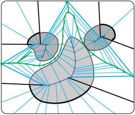
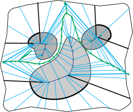
(a)                                                         (b)

Figure 25. a) Bounding box with curved corners containing a configuration of three regions and b) (a priori given) intrinsic bounding region for the same configuration. The linking structure is either extended to the boundary (in the region bounded by the darker lines on the boundary for $M_{i\,\infty}$) or truncated at the boundary.

Convex Hull:

The smallest convex region which contains a configuration is the convex hull of the configuration. For a generic configuration, the convex hull consists of the regions $\mathcal{B}_{i\,\infty}$ together with the truncated envelope of the family of degenerate supporting hyperplanes which meet the configuration with a degenerate tangency or at multiple points.

For a) of Figure 12 in § 4, which is a configuration in ${\mathbb{R}}^{2}$, the envelope consists of line segments joining the doubly tangent points corresponding to the points in the spherical axis (b) of Figure 12.

In ${\mathbb{R}}^{3}$, the envelope consists of a triangular portion of a triply tangent plane, with line segments joining pairs of points with a bitangent supporting plane, and a decreasing family of segments ending at a degenerate point (see Example 4.10 in § 4).

Intrinsic Bounding Region:

If the configuration is naturally contained in an (a priori given) intrinsic region, which is modeled by $\tilde{\Omega}$, then provided that the extensions of the radial lines intersect $\partial\tilde{\Omega}$ transversely, then we can modify the linking structure as in the convex case to have it defined on all of the $M_{i}$, and terminating at $\partial\tilde{\Omega}$, if linking has not already occurred (see e.g. Figure 25 (b)).

Threshold for Linking:

The external region can be bounded by placing a threshold $\tau$ on the $\ell_{i}$ so that the $L_{i}$ remain in a bounded region. This can be done in two different ways. An absolute threshold restricts the external regions to those arising from linking vector fields with $\ell_{i}\leq\tau$; and a truncated threshold restricts to a bounded region formed by replacing $\ell_{i}$ by $\ell_{i}^{\prime}=\min\{\ell_{i},\tau\}$. For the first type, only part of the region would have an external linking neighborhood; while in the second, the entire region would. As for the convex case, since we are replacing $\ell_{i}$ by smaller values, the linking flow will remain nonsingular. We obtain modified versions of the regions lying in a bounded region (see e.g. Figures 24 or 27).

Remark 9.3.

If the configuration is subjected to a transformation formed from a translation, rotation, and scaling, then we would like the associated bounded region $\tilde{\Omega}$ to be sent to the corresponding bounded region for the resulting image configuration. Provided we also scale the length of vectors, a skeletal linking structure will be sent by such mappings to a skeletal linking structure for the image configuration. This is also true for a Blum linking structure. Thus, it is only necessary that the associated bounding region is constructed from geometric data from the configuration. For the convex hull this is true. For an intrinsic bounding region, we would require that the transformations send one intrinsic bounding region to another. This will also happen for bounding boxes, etc or thresholds provided any reference points, directions of edges, and lengths are determined by the configuration.

10. Global Geometry via Medial and Skeletal Linking Integrals

We are now ready to use the regions we have defined for a configuration to introduce quantitative invariants measuring positional geometry for configurations. We do so in terms of integrals which are defined on the skeletal sets for the individual regions using the shape operators defined from the linking structure.

Defining Medial and Skeletal Linking Integrals

We begin by considering a medial or skeletal linking structure $\{(M_{i},U_{i},\ell_{i})\}$ for a multi-region configuration $\boldsymbol{\Omega}=\{\Omega_{i}\}$ in ${\mathbb{R}}^{n+1}$. We recall from §3 that we introduced the notation that $M=\coprod_{i>0}M_{i}$ denotes the disjoint union of the $M_{i}$ for each region $\Omega_{i}$ for $i>0$. Each $M_{i}$ has its double $\tilde{M}_{i}$, and we also introduced the double $\tilde{M}$ for the configuration by $\tilde{M}=\coprod_{i>0}\tilde{M}_{i}$. For each $i>0$, there is a canonical finite-to-one projection $\pi_{i}:\tilde{M}_{i}\to M_{i}$, mapping $(x,U(x))\mapsto x$. The union of these defines a canonical projection $\pi:\tilde{M}\to M$, such that $\pi|\tilde{M}_{i}=\pi_{i}$ for each $i>0$.

Even though $\boldsymbol{\Omega}$ is defined via an embedding $\Phi:\boldsymbol{\Delta}\to{\mathbb{R}}^{n+1}$, we will define the integrals directly using the skeletal linking structure for $\boldsymbol{\Omega}$. We will define the skeletal integral on $\tilde{M}$ for a multi-valued function $g:M\to{\mathbb{R}}$, by which we mean for any $x\in M_{i}$, $g$ may have a different value for each different value of $U_{i}$ at $x$. Such a $g$ pulls-back via $\pi$ to a well-defined map $\tilde{g}:\tilde{M}\to{\mathbb{R}}$ so that $g\circ\pi=\tilde{g}$.

To define the integrals we use an especially suited positive Borel measure on $\tilde{M}$. The Borel measures are defined separately for each $\tilde{M}_{i}$ and then together they give the Borel measure on $\tilde{M}$. The existence of the corresponding positive Borel measures $dM_{i}$ on each $\tilde{M}_{i}$ for each $i>0$ follows from Proposition 3.2 of [D4]. We briefly recall how they are defined. We cover $M_{i}$ by a finite union of paved neighborhoods $\{W_{k}\}$. We recall from §3 (see also [D4, §3]) that for a “paved neighborhood”  we mean an open $W_{k}$ whose closure may be decomposed into a finite number of connected smooth manifolds with boundaries and corners $M_{\alpha_{j}}$ which only meet along boundary facets, see e.g. Figure 6, and each value of $U$ is defined smoothly on $M_{\alpha_{j}}$.

The measure is defined by defining the integrals of continuous functions on $\tilde{M}$ and using the Riesz representation theorem. By a partition of unity argument as in e.g. [LS, Chap. 10] or [Sp, Vol. 1, Chap. 8], it is enough to define the integral for one such region $M_{\alpha_{j}}$. We let $M_{\alpha_{j}}^{(k)}$, $k=1,2$, denote the inverse images of $M_{\alpha_{j}}$ under the canonical projection map $\pi_{i}:\tilde{M}_{i}\to M_{i}$. Each $M_{\alpha_{j}}^{(k)}$ is a copy of $M_{\alpha_{j}}$, with the smooth value of $U_{i}$ associated to the copy. For each copy we let $dM_{j\,i}=\rho_{j\,i}dV_{i}$, where $dV_{i}$ is the Riemannian volume on $M_{\alpha_{j}}$ and $\rho_{j\,i}=\mathbf{u}_{k\,j}\cdot\mathbf{n}_{k\,j}$ where $\mathbf{u}_{k\,j}$ is a value of the unit vector field corresponding to the smooth value of $U_{k\,j}$ for $M_{\alpha_{j}}^{(k)}$ and $\mathbf{n}_{k\,j}$ is the normal unit vector pointing on the same side as $U_{k\,j}$.

By a partition of unity argument, we obtain integrals of continuous functions $\tilde{h}$ on $\tilde{M}_{i}$. Then, by the Riesz representation theorem, there is a regular positive Borel measure $dM_{i}$ on $\tilde{M}_{i}$ so that integration extends to Borel measurable functions $\tilde{h}$ on $\tilde{M}_{i}$, given by the integral with respect to this measure, see [D4, §3].

Then, for a multivalued function $g$ on $M_{\alpha_{j}}$, the integral of $g$ is, by definition, the sum of the integrals of the corresponding values of $g$ over each copy $M_{\alpha_{j}}^{(k)}$ with respect to the medial measure $dM_{k\,j}$. For Borel measurable functions $\tilde{g}$ on $\tilde{M}_{i}$ obtained (as above) by composing $g$ with $\pi_{i}$, this gives a well-defined integral with respect to the Borel measure $dM_{i}$ on $\tilde{M}_{i}$.

Then, the distinct Borel measures on $dM_{i}$ on $\tilde{M}_{i}$ together define a regular positive Borel measure $dM$ on $\tilde{M}$; and the integral of a Borel measurable multi-valued function $g$ on $M$ is defined to be

(10.1) $$\int_{\tilde{M}}g\,dM\,\,=\,\,\sum_{i>0}\int_{\tilde{M}_{i}}\tilde{g}\,dM_{i},$$

where each integral on the RHS is the integral of $\tilde{g}$ over $\tilde{M}_{i}$ with respect to the Borel measure $dM_{i}$, and it can be viewed as an integral of $g$ over “both sides of $M_{i}$”.

A Blum medial linking structure for a configuration of disjoint regions is itself a skeletal structure, so the integral makes sense for such configurations. We refer to the integrals in (10.1) as medial or skeletal linking integrals, depending on whether the linking structure is a Blum medial linking structure or a skeletal linking structure.

In the results that follow, just as in the preceding definition, we will be adapting the arguments given in [D4] for a single region to the individual regions of the configuration. Consequently, we will frequently outline the arguments and refer to the specific proofs in [D4] for the details.

Blum Medial Linking Integrals for General Configurations

For a general configuration with a full Blum linking structure, the Blum medial axis extends to the boundary; and its closure contains the edge-corner points of each $\Omega_{i}$. We briefly explain how the preceding definition of the integral can be extended to this case. We now include the edge-corner points as points of the medial axis $M_{i}$, so that it is still compact. The double $\tilde{M}_{i}$ is defined as before, except that there is only a single point lying over each edge-corner point, just as for the edge points of the medial axis in the smooth case. Again $\tilde{M}_{i}$ is a compact (and locally compact) Hausdorff space. Also, because there is the edge-corner normal form for the medial axis in the neighborhood of any edge-corner point, we can again give a paved neighborhood of any such point, in the sense of [D4, §3].

We can then define an integral of a multi-valued function $g$ on $M_{i}$ just as for skeletal structures using a partition of unity and paved neighborhoods. As in the preceding, there is a unique regular positive Borel measure $dM_{i}$ on $\tilde{M}_{i}$ so that the integral of $g$ on $M_{i}$ is the integral of $\tilde{g}$ with respect to the measure $dM_{i}$ on $\tilde{M}_{i}$. We shall refer to this measure as the skeletal (or medial) measure on $\tilde{M}_{i}$. Locally the measure still has the form $dM_{i}=\rho_{i}dV_{i}$, except now $\rho_{i}$ vanishes on the edge-corner points. In this case, we still refer to the integrals in (10.1) as medial linking integrals.

Computing Boundary Integrals via Medial Linking Integrals

So far the integrals which we have just defined only depend on the skeletal structures for the individual regions. We now show how, by using the linking flow, we may express integrals of functions on $\mathcal{B}$ or functions on ${\mathbb{R}}^{n+1}$ as medial or skeletal integrals over the skeletal sets.

Representing Integrals of Functions on $\mathcal{B}$ as Medial Integrals

First, we consider a Borel measurable function $g:\mathcal{B}\to{\mathbb{R}}$, integrable for volume measure on $\mathcal{B}$, which is allowed to be multi-valued in the sense that for any $k$-edge-corner point $x\in\mathcal{B}$, $g$ may take distinct values for each region $\Omega_{i}$, $i>0$, containing $x$ on its boundary. Thus, for a shared boundary region $\mathcal{B}_{i\,j}=\mathcal{B}_{i}\cap\mathcal{B}_{j}$, $g$ may take different values for each region $\Omega_{i}$ or $\Omega_{j}$ (so the values on $\mathcal{B}_{i\,j}$ for each $\Omega_{i}$ define a Borel measurable and integrable function on $\mathcal{B}_{i\,j}$ and on $\mathcal{B}_{i\,0}=\mathcal{B}_{i}\backslash\cup_{j\neq i}\mathcal{B}_{j}$). For example, such a function might represent a physical quantity such as a density of the boundary region which may differ for each region $\Omega_{i}$ and hence give two possible values on shared regions such as $\mathcal{B}_{i\,j}$. By the integral of such a multi-valued function $g$ over $\mathcal{B}$ we mean

$$\int_{\mathcal{B}}g\,dV\,\,=\,\,\sum_{i\neq j,\,i,j\geq 0}\int_{\mathcal{B}_{i\,j}}g_{i\,j}\,dV$$

where $g_{i\,j}$ denotes the values of $g$ on $\mathcal{B}_{i\,j}$ for $\Omega_{i}$ and $dV$ denotes the $n$-dimensional Riemannian volume on each $\mathcal{B}_{i}$. This includes both $\mathcal{B}_{i\,0}$ and $\mathcal{B}_{i\,\infty}$ so the integral is over the complete boundaries of all regions.

Then, for the time-one radial flow map $\psi_{i\,1}:\tilde{M}_{i}\to\mathcal{B}_{i}$, we define $\tilde{g}:M_{i}\to{\mathbb{R}}$ by $\tilde{g}=g\circ\psi_{i\,1}$, where the value on $\mathcal{B}_{i\,j}$ is the value associated to $\Omega_{i}$. Then, $\tilde{g}$ is a multi-valued Borel measurable function on $M_{i}$.

We may compute the integral of $g$ over $\mathcal{B}$ by the following result.

Theorem 10.1.

Let $\boldsymbol{\Omega}$ be a multi-region configuration with (full) Blum linking structure. If $g:\mathcal{B}\to{\mathbb{R}}$ is a multi-valued Borel measurable and integrable function, then

(10.2) $$\int_{\mathcal{B}}g\,dV\,\,=\,\,\int_{\tilde{M}}\tilde{g}\det(I-r_{i}S_{rad})\,dM\,$$

where $r_{i}$ is the radius function of each $\tilde{M}_{i}$.

Proof.

In the case of a configuration of disjoint regions with smooth boundaries, for each region $\Omega_{i}$, $g$ is a well-defined function on $\mathcal{B}_{i}$ and we may apply Theorem 4.1 of [D4] to conclude

(10.3) $$\int_{\mathcal{B}_{i}}g\,dV\,\,=\,\,\int_{\tilde{M}_{i}}\tilde{g}\det(I-r_{i}S_{rad})\,dM_{i}\,.$$

Summing (10.3) over $i>0$ gives the result in this case.

Next for a general configuration, we first consider a single region $\Omega_{i}$ in it. We may apply the proof of [D4, Thm 4.1] to one of the regions $M_{i\,\alpha}$ with a given smooth value of $U_{i}$ on it. If $M_{i\,\alpha}$ meets the edge-corner strata, it does so on its boundary. Let $B_{i\,\alpha}^{(j)}=\psi_{i\,1}(M_{i\,\alpha}^{(j)})$ for the given values for $U_{i}$. Then, $\psi_{i\,1}|M_{i\,\alpha}^{(j)}$ is a homeomorphism to $B_{i\,\alpha}^{(j)}$, and $\psi_{i\,1}$ is nonsingular on the interior of $M_{i\,\alpha}$. Thus, we can still apply the change of variables formula for multiple integrals. Hence, applying the proof of [D4, Thm 4.1] we obtain

(10.4) $$\int_{B_{i\,\alpha}}g\,dV\,\,=\,\,\int_{\tilde{M}_{i\,\alpha}}\tilde{g}\det(I-r_{i}S_{rad})\,dM_{i}\,.$$

Then, we can first sum (10.4) over the $M_{i\,\alpha}^{(j)}$ which form a paved neighborhood, to obtain the result on paved neighborhoods, and then use the partition of unity to obtain (10.3). ∎

In the case of a skeletal structure, there is a form of Theorem 10.1 which still applies. For each region $\Omega_{i}$, with $i>0$, let $\tilde{R}_{i}$ denote a Borel measurable region of $\tilde{M}_{i}$ which under the radial flow maps to a Borel measurable region $R_{i}$ of $\mathcal{B}_{i}$. Let $R=\cup_{i}R_{i}$ and $\tilde{R}=\cup_{i}\tilde{R}_{i}$. We suppose that the skeletal structure satisfies the “partial Blum condition”  on $\tilde{R}$, by which we mean: for each $i$, the compatibility $1$-form $\eta_{U_{i}}$ vanishes on $\tilde{R}_{i}$ (recall this means that the radial vector $U_{i}$ at points of $x\in\tilde{R}_{i}$ is orthogonal to $\mathcal{B}_{i}$ at the point where it meets the boundary). Note that for a skeletal structure this forces $R$ to be contained in the complement of $\mathcal{B}_{sing}$.

Then, there is the following analogue of Theorem 10.1.

Corollary 10.2.

Let $\boldsymbol{\Omega}$ be a multi-region configuration with skeletal linking structure which satisfies the partial Blum condition on the region $\tilde{R}\subset\tilde{M}$, with image $R$ under $\psi_{1}$. If $g:R\to{\mathbb{R}}$ is a multi-valued Borel measurable and integrable function, then

(10.5) $$\int_{R}g\,dV\,\,=\,\,\int_{\widetilde{R}}\tilde{g}\det(I-r_{i}S_{rad})\,dM\,.$$

Proof.

We again follow the proof of Theorem 4.1 in [D4]. We let $\chi_{R}$ denote the characteristic function of the region $R$ on $\mathcal{B}$ (so it equals $1$ on $R$ and $0$ off $R$), and we replace $g$ by $g^{\prime}=\chi_{R}\cdot g$. Then the integral of $g$ over $R$ equals that of $g^{\prime}$ over $\mathcal{B}$.

We may cover $R$ by paved neighborhoods whose images lie in the smooth strata of $\mathcal{B}$, and paved neighborhoods which miss $R$. For each $M_{i\,\alpha}^{(j)}$ which appears in one of the paved neighborhoods meeting $R$, we apply the proof of Theorem 4.1 in [D4]. By the partial Blum condition $U_{i}^{(j)}$ is normal to $\mathcal{B}_{i\,\alpha}^{(j)}$ at $\psi_{i\,1}(x)$ for $x\in\tilde{R}\cap M_{i\,\alpha}^{(j)}$; thus

$$g^{\prime}\,d\psi_{i\,1}^{*}(dV)\,\,=\,\,\begin{cases}0&x\notin\tilde{R},\\ \tilde{g}\det(I-r_{i}S_{rad})\,dM&x\in\tilde{R}.\end{cases}$$

Thus,

(10.6) $$\int_{R\cap\mathcal{B}_{i\,\alpha}^{(j)}}g\,dV\,\,=\,\,\int_{\widetilde{R}\cap M_{i\,\alpha}^{(j)}}\tilde{g}\det(I-r_{i}S_{rad})\,dM\,,$$

yielding the result on $M_{i\,\alpha}^{(j)}$. Then, we may follow the reasoning in the proof of [D4, Thm. 4.1] to obtain the conclusion. ∎

Volumes of Regions in $\mathcal{B}$

We give one application of Theorem 10.1 to computing the $n$-dimensional volume of $\mathcal{B}$. There are two possible meanings for this. The “complete volume”  includes the volume of each $\mathcal{B}_{i}$, counting that of each shared boundary $\mathcal{B}_{i\,j}$ for both $\mathcal{B}_{i}$ and $\mathcal{B}_{j}$. The other “partial volume”counts the shared boundaries only once. We may compute the complete volume by applying Theorem 10.1 to $g\equiv 1$.

Corollary 10.3.

Let $\boldsymbol{\Omega}$ be a multi-region configuration with (full) Blum medial linking structure. Then the complete volume of $\mathcal{B}$ is given by

(10.7) $$\text{complete $n$-dim ${\rm vol}\,(\mathcal{B})$}\,\,=\,\,\int_{\tilde{M}}\det(I-r_{i}S_{rad})\,dM\,.$$

$\Box$

For the partial volume, we linearly order the boundaries $\mathcal{B}_{i}$, letting “$\succ$”  denote the ordering, and define the multi-valued function $\check{1}$ on $\mathcal{B}$ so that for $\mathcal{B}_{i}$, $\check{1}$ equals $1$ except on the strata $\mathcal{B}_{i\,j}$ with $\mathcal{B}_{j}\succ\mathcal{B}_{i}$, where instead it equals $0$. This is the characteristic function for a region in $\mathcal{B}$ that corresponds under the radial flow to a region $\check{M}\subset\tilde{M}$, which is the union of $\check{M}_{i}\subset\tilde{M}_{i}$. Thus, by applying Theorem 10.1 to $\check{1}$ we obtain the following.

Corollary 10.4.

Let $\boldsymbol{\Omega}$ be a multi-region configuration with (full) Blum medial linking structure. Then, the partial volume of $\mathcal{B}$ is given by

(10.8) $$\text{partial $n$-dim ${\rm vol}\,(\mathcal{B})$}\,\,=\,\,\int_{\check{M}}\det(I-r_{i}S_{rad})\,dM\,.$$

$\Box$

Remark 10.5.

There is an analogous result for a region $R\subset\mathcal{B}$ which is the image of a region $\tilde{R}\subset\tilde{M}$ under the radial flow. If the configuration is modeled by a skeletal linking structure which satisfies the partial Blum condition on $\tilde{R}$, then the (complete) volume of $R$ is given by $\int_{\tilde{R}}\det(I-r_{i}S_{rad})\,dM$.

We may expand $\det(I-tS_{rad})=\sum_{j=0}^{n}(-1)^{j}\sigma_{j}t^{j}$, where $\sigma_{j}$ is the $j$-th elementary symmetric function in the principal radial curvatures $\kappa_{i}$. Applying the formulas, we may write the integrals as a sum of integrals $(-1)^{j}\int\tilde{g}\sigma_{j}\,r_{i}^{j}\,dM$, which are “moment integrals”  of the functions $\tilde{g}\sigma_{j}$ with respect to the radial functions. Examples of these explicit integrals for a single region can be found in [D4, §6.1]; for configurations of regions the integrands have the same forms.

Computing Integrals as Skeletal Linking Integrals via the Linking Flow

Next we turn to the problem of computing integrals over regions which may be partially or completely in the external region of the configuration. Quite generally we consider a Borel measurable and Lebesgue integrable function $g:{\mathbb{R}}^{n+1}\to{\mathbb{R}}$ with compact support. We shall see that we can compute the integral of $g$ as a skeletal linking integral of an appropriate related function.

Since we are in the unbounded case, we first modify the skeletal linking structure by defining $\ell_{i}$ on $M_{i\,\infty}$ to be $\ell_{i}=\infty$. By Proposition 14.11, the linking flow on $M_{i\,\infty}$ is a diffeomorphism for $0\leq t<\infty(=\ell_{i})$.

Next, we first replace the linking flow by a simpler elementary linking flow defined by $\lambda^{\prime}_{t}(x)=x+t\mathbf{u}_{i}$, for $0\leq t\leq\ell_{i}$ (or $<\infty$ if $\ell_{i}=\infty$). The elementary linking flow is again along the lines determined by the linking vector field $L_{i}$; however, the rate of flow differs from that for the usual linking flow. This means that the level surfaces will differ, although the image of strata under the elementary linking flow agrees with that for the linking flow. In addition, as the linking flow is nonsingular, Proposition 8.1 implies that the linking curvature and edge conditions are satisfied. Then, for the linking vector field, viewed as a radial vector field, the radial curvature and edge curvature conditions are satisfied, and hence imply the nonsingularity of the elementary linking flow.

Then, using the elementary linking flow, we can compute the integral of $g$ as a skeletal linking integral. We define a multi-valued function $\tilde{g}$ on $M$ as follows: for $x\in M_{i}$ with associated smooth value $U_{i}$ and linking vector $L_{i}$ in the same direction as $U_{i}$ (so $(x,U_{i})\in\tilde{M}_{i}$),

(10.9) $$\tilde{g}(x)\,\,\overset{def}{=}\,\,\int_{0}^{\ell_{i}}g(\lambda^{\prime}_{t}(x))\det(I-tS_{rad})\,dt$$

provided the integral is defined. Then, we have the following formula for the integral of $g$ as a skeletal linking integral.

Theorem 10.6.

Let $\boldsymbol{\Omega}$ be a multi-region configuration in ${\mathbb{R}}^{n+1}$ with a skeletal linking structure. If $g:{\mathbb{R}}^{n+1}\to{\mathbb{R}}$ is a Borel measurable and Lebesgue integrable function with compact support, then $\tilde{g}(x)$ is defined for almost all $x\in\tilde{M}$, it is integrable on $\tilde{M}$, and

(10.10) $$\int_{{\mathbb{R}}^{n+1}}g\,dV\,\,=\,\,\int_{\tilde{M}}\tilde{g}\,dM\,.$$

Remark 10.7.

If we compare this formula with that given for a single region in Theorem 6.1 of [D4], we notice they have a slightly different form. However, as noted in Remark 6.2 of that paper, it is possible to use a change of coordinates $t^{\prime}=\ell_{i}t$ to rewrite

(10.11) $$\tilde{g}(x)\,\,=\,\,\ell_{i}\int_{0}^{1}g(x+t^{\prime}L_{i})\det(I-t^{\prime}\ell_{i}S_{rad})\,dt^{\prime}\,,$$

which agrees with the form given there. We will use the same change of coordinates to rewrite the formula differently below. In proving the theorem we will find it useful to first reduce it to the integral for a modified linking structure over a bounded region.

Reducing to Integrals for Bounded Skeletal Linking Structures

We relate the unbounded skeletal structure to a bounded one. We let $Q={\rm supp}\,(g)$, which is compact. We may find a compact convex region $\tilde{\Omega}$ with smooth boundary containing both the configuration $\boldsymbol{\Omega}$ and $Q$. Then, we can modify the linking structure by reducing the $L_{i}$ so it is truncated by $\partial\tilde{\Omega}$ and defining $L_{i}$ on $M_{i\,\infty}$ as the extensions of the radial vectors to where they meet $\partial\tilde{\Omega}$. Because the extended radial lines are transverse to $\partial\tilde{\Omega}$, the new values of $\ell_{i}$, which we denote by $\ell_{i}^{\prime}$, remain smooth on the strata of each $M_{i}$. We also let $L_{i}^{\prime}=\ell_{i}^{\prime}\mathbf{u}_{i}$, with $\mathbf{u}_{i}$ denoting the unit vector in the same direction as $L_{i}$, be the corresponding linking vector. As $\ell_{i}^{\prime}\leq\ell_{i}$, the linking flow remains nonsingular on all strata of $\tilde{M}$.

First, we may express

(10.12) $$\int_{{\mathbb{R}}^{n+1}}\,g\,dV\,\,=\,\,\int_{\tilde{\Omega}}\,g\,dV$$

This allows us to reduce the proof of Theorem 10.6 to the case of the bounded integral on the RHS of (10.12) using the bounded linking structure on $\tilde{\Omega}$.

Proof of Theorem 10.6.

For the proof, we first also reduce the integral on the RHS of (10.10) as an integral over the bounded region. Since the intersection of ${\rm supp}\,(g)$ with the linking line segment $\{t\mathbf{u}_{i}:0\leq t<\ell_{i}\}$ lies in $\{t\mathbf{u}_{i}:0\leq t<\ell_{i}^{\prime}\}$,

(10.13) $$\tilde{g}(x)\,\,=\,\,\int_{0}^{\ell_{i}^{\prime}}g(\lambda^{\prime}_{t}(x))\det(I-tS_{rad})\,dt\,.$$

By the change of coordinates $t=\ell_{i}^{\prime}t^{\prime}$, we obtain

(10.14) $$\tilde{g}(x)\,\,=\,\,\ell_{i}^{\prime}\int_{0}^{1}g(x+t^{\prime}L_{i}^{\prime})\det(I-t^{\prime}\ell_{i}^{\prime}S_{rad})\,dt^{\prime}\,.$$

Then, (10.10) reduces to computing the integral in the RHS of (10.10) using the bounded structure as an integral of (10.14). Also, as the elementary linking flow is still one-one on each linking line, the elementary linking flow $\lambda_{i}^{\prime}$ is still a homeomorphism on any of the regions $M_{i\,\alpha}^{(j)}$. Also, by the preceding discussion the elementary linking flow is also nonsingular on the interior of $M_{i\,\alpha}^{(j)}\times[0,1]$ with image in ${\mathbb{R}}^{n+1}$, denoted $R_{i\,\alpha}^{(j)}$. Thus, using the change of variables formula for multiple integrals and the argument proving Theorem 6.1 in [D4], we obtain

(10.15) $$\int_{R_{i\,\alpha}^{(j)}}\,g\,dV\,\,=\,\,\int_{M_{i\,\alpha}^{(j)}}\tilde{g}(x)\,dt^{\prime}\,.$$

where $\tilde{g}(x)$ is given by (10.14), which is the same as (10.9).

Thus, we may follow the reasoning from the proof of Theorem 6.1 in [D4] to complete the proof. ∎

As an immediate consequence of Theorem 10.6 we can deduce the following. Let

$$g_{Q}(x)=\int_{0}^{\ell_{i}^{\prime}}g(\lambda_{t}^{\prime}(x))\chi_{Q}(\lambda_{t}^{\prime}(x))\det(I-tS_{rad,i})\,dt\,.$$

Corollary 10.8.

Let $\boldsymbol{\Omega}$ be a multi-region configuration with skeletal linking structure. Suppose that $Q\subset{\mathbb{R}}^{n+1}$ is a compact subset and $g:{\mathbb{R}}^{n+1}\to{\mathbb{R}}$ is a Borel measurable and Lebesque integrable function on $Q$. Then,

(10.16) $$\int_{Q}\,g\,dV\,\,=\,\,\int_{\tilde{M}}g_{Q}\,dM\,.$$

The proof is an immediate consequence of Theorem 10.6 applied to $\chi_{Q}\cdot g$.  $\Box$

In the special case where $g\equiv 1$, we obtain an analogue of the Crofton formula. For a compact subset $Q\subset{\mathbb{R}}^{n+1}$ and each $x\in\tilde{M}_{i}$, we define the multi-valued function

$$m_{Q}(x)\,\,=\,\,\int_{0}^{\ell_{i}}\chi_{Q}(x+tL_{i}(x))\det(I-tS_{rad})\,dt\,.$$

We can view $m_{Q}(x)$ as a weighted $1$-dimensional measure of the intersection of $Q$ with the linking line from $x$ determined by $L_{i}(x)$.

Corollary 10.9 (Crofton Type Formula).

Let $\boldsymbol{\Omega}$ be a multi-region configuration with skeletal linking structure. Suppose $Q\subset{\mathbb{R}}^{n+1}$ is a compact subset. Then,

(10.17) $${\rm vol}\,(Q)\,\,=\,\,\int_{\tilde{M}}m_{Q}(x)\,dM\,.$$

$\Box$

Decomposition of a Global Integral using the Linking Flow

We next decompose the integral on the RHS of (10.16) using the alternative integral representation of $\tilde{g}$ using the linking flow. We do so by applying the change of variables formula to relate the elementary linking flow $\lambda^{\prime}$ with the linking flow $\lambda$, both of which flow along the linking lines but at different linear rates.

We define

$$\tilde{g}_{int}(x)\,\, =\,\,\int_{0}^{r_{i}}g(x+t\mathbf{u}_{i})\det(I-tS_{rad})\,dt\,\quad\text{ and }\quad$$

(10.18) $$\tilde{g}_{ext}(x)\,\, =\,\,\int_{r_{i}}^{\ell_{i}}g(x+t\mathbf{u}_{i})\det(I-tS_{rad})\,dt.$$

These may be alternately written using a change of coordinates as

(10.19) $$\tilde{g}_{int}(x)\,\,=\,\,r_{i}\int_{0}^{1}g(x+tr_{i}\mathbf{u}_{i})\det(I-tr_{i}S_{rad})\,dt\,.$$

and

(10.20) $$\tilde{g}_{ext}(x)\,\,=\,\,(\ell_{i}-r_{i})\int_{0}^{1}g(x+(r_{i}+t(\ell_{i}-r_{i}))\mathbf{u}_{i})\det(I-(r_{i}+t(\ell_{i}-r_{i}))S_{rad})\,dt\,.$$

Then, we may decompose $\int g$ as follows.

Corollary 10.10.

Let $\boldsymbol{\Omega}$ be a multi-region configuration in ${\mathbb{R}}^{n+1}$ with a skeletal linking structure. If $g:{\mathbb{R}}^{n+1}\to{\mathbb{R}}$ is a Borel measurable and Lebesgue integrable function with compact support, then, $\tilde{g}_{int}(x)$ and $\tilde{g}_{ext}(x)$ are defined for almost all $x\in\tilde{M}$, they are integrable on $\tilde{M}$, and

(10.21) $$\int_{{\mathbb{R}}^{n+1}}g\,dV\,\,=\,\,\int_{\tilde{M}}\tilde{g}_{int}\,dM\,\,+\,\,\int_{\tilde{M}}\tilde{g}_{ext}\,dM\,,$$

where

(10.22) $$\int_{\tilde{M}}\tilde{g}_{int}\,dM\,\,=\,\,\sum_{i,j>0}\int_{M_{i\to j}}\tilde{g}_{int}\,dM\,\,+\,\,\sum_{i>0}\int_{M_{i\,\infty}}\tilde{g}_{int}\,dM\,,$$

with an analogous formula with $g_{int}$ replaced by $g_{ext}$ everywhere in (10.22).

The first integral on the RHS of (10.21) is the “interior integral”  of $g$ within the configuration using the radial flow, and the second integral is the“external integral”  computed using the linking flow outside of the configuration. Then we may decompose each of these integrals using (10.22) into integrals over the distinct linking regions as illustrated in Figure 26

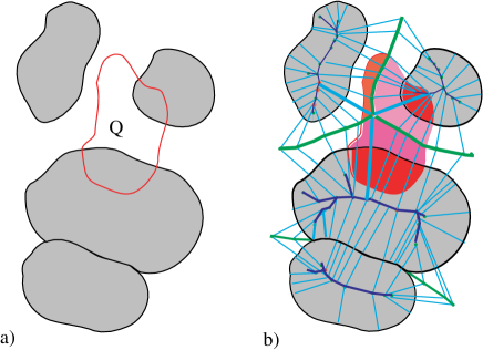
Figure 26. The decomposition of the integral over a region $Q$ outlined in a) is given as the sum of integrals over regions in b) obtained by the subdivision of $Q$ by the linking axis and the three linking lines to the branch point of the linking axis. Each $Q_{i\,j}\subset\mathcal{R}_{i\to j}$ (or in general including $Q_{i\,\infty}\subset\mathcal{R}_{i\,\infty}$) in the figure consists of the darker region inside the subregion $\Omega_{i\to j}$ together with the portion of $Q$ in the linking neighborhood $\mathcal{N}_{i\to j}$. The integral can then be expressed by Corollary 10.10 as sums of internal and external integrals over the $M_{i\to j}$ and $M_{i\,\infty}$.

Proof.

For (10.21) we may just apply Theorem 10.6 and compute the RHS of (10.11) as a sum of two integrals by writing (10.9) as a sum of two integrals to obtain $\tilde{g}=\tilde{g}_{int}+\tilde{g}_{ext}$. That they are defined for almost all $x\in\tilde{M}$ follows from an application of Fubini’s Theorem as in the proof of Theorem 6.1 in [D4]. This decomposes the linking flow into the parts both before and after the flow reaches the boundary.

For (10.22), we use that $\tilde{M}$ is a union of $M_{i\to j}$ for $i,j>0$ and $M_{i\,\infty}$ for $i>0$. These are unions of strata which form $n$-dimensional stratified sets, and hence are Borel sets of dimension $n$. Also, any two of these intersect on a union of strata of dimension $<n$ which have measure $0$ in $\tilde{M}$. Thus,

$$\int_{\tilde{M}}g_{int}\,dV\,\,=\,\,\sum_{i,j>0}\int_{M_{i\to j}}g_{int}\,dV\,\,+\,\,\sum_{i>0}\int_{M_{i\,\infty}}g_{int}\,dM\,.$$

This yields (10.22) with an analogous formula for $g_{ext}$. ∎

Skeletal Linking Integral Formulas for Global Invariants

We now express the volumes of regions associated to the linking structure as skeletal linking integrals. We may apply the same reasoning as in Corollary 10.9, using Corollary 10.10 to compute the volumes of compact measurable regions $Q\subset{\mathbb{R}}^{n+1}$ as a sum of internal and external integrals. We consider a specific application for linking regions.

For these calculations we will use the expression

(10.23) $$\mathcal{I}(t)\,\,\overset{def}{=}\,\,\int_{0}^{t}\det(I-tS_{rad})\,dt\,\,=\,\,\sum_{j=0}^{n}\frac{(-1)^{j}}{j+1}\sigma_{j}t^{j+1}\,.$$

Volumes of Linking Regions as Skeletal Integrals

We consider a multi-region configuration with a bounded skeletal linking structure.

Corollary 10.11.

Let $\boldsymbol{\Omega}\subset\tilde{\Omega}$ be a multi-region configuration with a bounded skeletal linking structure. Then,

$${\rm vol}\,(\mathcal{N}_{i\to j})\,\, =\,\,\int_{\tilde{M}_{i\to j}}\mathcal{I}(\ell_{i})-\mathcal{I}(r_{i})\,dM\,\quad\text{ and }\quad{\rm vol}\,(\Omega_{i\to j})\,\, =\,\,\int_{M_{i\to j}}\mathcal{I}(r_{i})\,dM\,$$

(10.24) $${\rm vol}\,(\mathcal{N}_{i\,\infty})\,\, =\,\,\int_{M_{i\,\infty}}\mathcal{I}(\ell_{i})-\mathcal{I}(r_{i})\,dM\,\quad\text{ and }\quad{\rm vol}\,(\Omega_{i\,\infty})\,\, =\,\,\int_{M_{i\,\infty}}\mathcal{I}(r_{i})\,dM\,.$$

It then follows that we can compute the volumetric invariants of the various linking regions such as $\mathcal{R}_{i\to j}$, $\mathcal{N}_{i}$, etc. using skeletal linking integrals of the polynomials $\mathcal{I}(\ell_{i})$ or $\mathcal{I}(r_{i})$. For example,

(10.25) $${\rm vol}\,(\mathcal{R}_{i\to j})=\int_{M_{i\to j}}\mathcal{I}(\ell_{i})\,dM\,,$$

with an analogous formula for ${\rm vol}\,(\mathcal{R}_{i\,\infty})$.

As a consequence, we obtain generalizations of both Weyl’s formula for volumes of tubes [W] and Steiner’s formula, see e.g. [Gr].

Corollary 10.12 (Generalized Weyl’s Formula).

Let $\boldsymbol{\Omega}\subset\tilde{\Omega}$ be a multi-region configuration with a bounded skeletal linking structure. Then,

(10.26) $${\rm vol}\,(\Omega_{i})\,\,=\,\,\int_{\tilde{M}_{i}}\mathcal{I}(r_{i})\,dM\,.$$

The sense in which this generalizes Weyl’s formula is explained for the case of a single region with smooth boundary in [D4, §6, 7]. For Steiner’s formula, we note that as explained in §9, $\mathcal{N}_{i}\cup\mathcal{N}_{i\to i}\cup\mathcal{N}_{i\,\infty}$ represents the total neighborhood of $\Omega_{i}$, which is the region about $\Omega_{i}$ extending along the linking lines. This is a generalization of a partial tubular neighborhood about a region which depends on the specific type of bounding region (see Figure 27).

Corollary 10.13 (Generalized Steiner’s Formula).

Let $\boldsymbol{\Omega}\subset\tilde{\Omega}$ be a multi-region configuration with a bounded skeletal linking structure. Then,

(10.27) $${\rm vol}\,(\mathcal{N}_{i}\cup\mathcal{N}_{i\to i}\cup\mathcal{N}_{i\,\infty})\,\,=\,\,\int_{\tilde{M}}\mathcal{I}(\ell_{i})-\mathcal{I}(r_{i})\,dM\,.$$

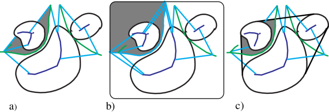
Figure 27. Examples of a total neighborhood $\mathcal{N}_{i}\cup\mathcal{N}_{i\to i}\cup\mathcal{N}_{i\,\infty}$ for a region $\Omega_{i}$, to which the generalized Steiner’s formula applies: a) absolute threshold; b) bounding box; and c) convex hull.

Both of these results are immediate consequences of Corollary 10.11.           $\Box$

Proof of Corollary 10.11.

In each case, it is sufficient to apply Corollary 10.10. For example, for $\mathcal{N}_{i\to j}$, we apply the theorem to $g=\chi_{\mathcal{N}_{i\to j}}$, whose integral equals ${\rm vol}\,(\mathcal{N}_{i\to j})$. The internal integral is zero and to compute the external integral, the characteristic function is $\equiv 1$ on the external part of the linking lines so we obtain using (10.23) that $\tilde{g}_{ext}=\mathcal{I}(\ell_{i})-\mathcal{I}(r_{i})$ at points of $M_{i\to j}$ and $0$ otherwise. Thus, the integral is as stated. ∎

We next turn to defining the positional geometric invariants in terms of volumes of regions.

11. Positional Geometric Properties of Multi-Region Configurations

We consider a configuration $\boldsymbol{\Omega}=\{\Omega_{i}\}\subset\tilde{\Omega}$, in the bounding region $\tilde{\Omega}$ with a bounded skeletal linking structure. We will now use the linking structure to investigate the positional geometry of the configuration. First, we use it to determine which of the regions should be regarded as neighboring regions. Then, we use the regions associated to the linking structure to define invariants which measure the closeness of such neighboring regions. We further introduce invariants measuring “positional significance”of regions for the configuration. These allow us to identify which regions are central to the configuration and which ones are peripheral. Then, we construct a tiered linking graph, with vertices representing the regions, and edges between neighboring regions, with the closeness and significance values assigned to the edges, resp. vertices. By applying threshold values to this structure we can exhibit the subconfigurations within the given thresholds.

We show that these invariants are unchanged under the action of the Euclidean group and scaling acting on the configuration and bounding region. Furthermore, because these invariants are defined in terms of volumes of regions associated to the linking structure, the results of the previous section allow us to compute them as skeletal linking integrals.

Neighboring Regions and Measures of Closeness

We begin by using previous results to identify neighboring regions and measuring their closeness. We use linking between regions as a criterion for their being neighbors. Then, a potential first measure of closeness would be to determine, for a fixed $\Omega_{i}$, the minimum value of the radial linking function $\ell_{i}$. If $\|L_{i}(x)\|$ is the value of $\ell_{i}$ at this minimum, then we determine any vector $L_{j}(x^{\prime})$ so that $x^{\prime}$ is linked to $x$, and conclude that $\Omega_{j}$ and $\Omega_{i}$ are in some sense close. However, it is possible that two regions are only a small distance away from one another at some point, so that $\|L_{i}(x)\|=\|L_{j}(x^{\prime})\|$ is small, but are otherwise at most points a much greater distance apart. By contrast, there may be a third region $\Omega_{k}$ whose linking vector of smallest norm linking $\Omega_{i}$ to $\Omega_{k}$ has larger norm than $\|L_{j}(x^{\prime})\|$, but possibly other nearby vectors of $L_{i}$ and $L_{k}$ maintain approximately the same length along a much greater region. Such a situation is illustrated in Figure 24 or 28, where $\Omega_{3}$ is close to $\Omega_{1}$ for a small region but $\Omega_{2}$ is close to $\Omega_{1}$ over a larger region.

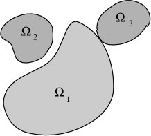
Figure 28. Measure of Closeness. Deciding whether $\Omega_{2}$ or $\Omega_{3}$ is “closer”to $\Omega_{1}$.

Thus, an appropriate measure of closeness should take into account how large is the external region where the regions are close, compared with the size of the regions themselves. We will do so by using volumetric measures of appropriate regions. For a configuration $\boldsymbol{\Omega}$ with a skeletal linking structure, we introduced in § 9, Definition 9.1, the regions $\Omega_{i\to j}$, $\mathcal{N}_{i\to j}$, and $\mathcal{R}_{i\to j}$. Because we will use volumetric measures of these regions, we assume that we have a bounded configuration $\boldsymbol{\Omega}=\{\Omega_{i}\}$ in a bounding region $\tilde{\Omega}$ with corresponding bounded skeletal linking structure. Thus, all of the regions will have finite volume.

The regions $\Omega_{i\to j}$ and $\Omega_{j\to i}$ capture the neighbor relations between $\Omega_{i}$ and $\Omega_{j}$. As we explained in §9, $\mathcal{N}_{i\to j}$ and $\mathcal{N}_{j\to i}$ share a common boundary region in $M_{0}$, so they are both empty if one is, and then both $\Omega_{i\to j}$ and $\Omega_{j\to i}$ are empty. In that case $\Omega_{i}$ and $\Omega_{j}$ are not linked. Otherwise, we may introduce a measure of closeness.

There are two different ways to do this, each having a probabilistic interpretation. First, we let

$$c_{i\to j}=\frac{{\rm vol}\,(\Omega_{i\to j})}{{\rm vol}\,(\mathcal{R}_{i\to j})}\qquad\text{ and }\qquad c_{i\,j}\,=\,c_{i\to j}\cdot c_{j\to i}\,.$$

Then, $c_{i\to j}$ is the probability that a point chosen at random in $\mathcal{R}_{i\to j}$ will lie in $\Omega_{i}$ (see Figure 29); so $c_{i\,j}$ is the probability that a pair of points, one each in $\mathcal{R}_{i\to j}$ and $\mathcal{R}_{j\to i}$ both lie in the corresponding regions $\Omega_{i}$ and $\Omega_{j}$.

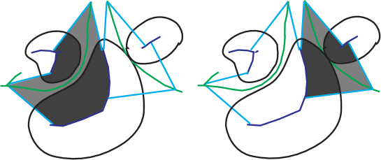
Figure 29. Measure of closeness for regions in the configuration in Figure 28 bounded via a threshold with the bounded skeletal linking structure (see § 9). For a pair of neighboring regions $\Omega_{i}$ and $\Omega_{j}$, $c_{i\to j}$ denotes the ratio of the volume of the darker region $vol(\Omega_{i\to j})$ and the volume of the total shaded region $vol(\mathcal{R}_{i\to j})=vol(\Omega_{i\to j})+vol(\mathcal{N}_{i\to j})$.

Note that $c_{i\,j}$ contains much more information than the closest distance between $\Omega_{i}$ and $\Omega_{j}$, and even the “$L^{1}$-measure”of the region between $\Omega_{i}$ and $\Omega_{j}$. It compares this measure with how much of the regions $\Omega_{i}$ and $\Omega_{j}$ are closest as neighbors. If both $\Omega_{i\to j}$ and $\Omega_{j\to i}$ are empty, we let $c_{i\to j}$, $c_{j\to i}$, and $c_{i\,j}=0$. Also, we let $c_{i\,i}=1$. Thus, from the collection of values $\{c_{i\,j}\}$ we can compare the closeness of any pair of regions.

Since these invariants depend on a bounded skeletal linking structure, one way to introduce a parametrized family $c_{i\,j}(\tau)$ is by considering the varying threshold values $\tau$. For example, $\tau$ may represent the maximum allowable values for $\ell_{i}$ or the maximum value of $\ell_{i}$ relative to some intrinsic geometric linear invariant of $\Omega_{i}$. As $\tau$ increases, the bounded region increases and how $c_{i\,j}(\tau)$ varies indicates how the closeness of the regions varies when larger linking values are taken into account.

A second way to introduce a measure of closeness is to use an “additive”contribution from each region and define

$$c_{i\,j}^{a}\,\,=\,\,\frac{{\rm vol}\,(\Omega_{i\to j})+{\rm vol}\,(\Omega_{j\to i})}{{\rm vol}\,(\mathcal{R}_{i\to j})+{\rm vol}\,(\mathcal{R}_{j\to i})}\,.$$

Here $c_{i\,j}^{a}$ is the probability that a point chosen in the region $\mathcal{R}_{i\to j}\cup\mathcal{R}_{j\to i}$ lies in the configuration, i.e. in $\Omega_{i}\cup\Omega_{j}$. We also let $c_{i\,j}^{a}=0$ if $\Omega_{i}$ and $\Omega_{j}$ are not linked; and we let $c_{i\,i}^{a}=1$. Again, to obtain a more precise measure of closeness, we can vary a measure of threshold $\tau$ and obtain a varying family $c_{i\,j}^{a}(\tau)$. The invariants satisfy $0\leq c_{i\,j},c_{i\,j}^{a}\leq 1$. The value $0$ indicates no linking, for values near $0$, the regions are neighbors but distant so they are “weakly linked”, and for values close to $1$, the regions are close over a large boundary region and are “strongly linked”.

There is a simple but crude relation between $c_{i\,j}^{a}$ and the pair $c_{i\to j}$ and $c_{j\to i}$:

$$c_{i\,j}^{a}\,\,\leq\,\,c_{i\to j}\,+\,c_{j\to i}\,.$$

As $c_{i\,j}^{a}\leq 1$, this is only useful when the two regions are weakly linked. This inequality is a special case of the following simple lemma whose proof follows easily by induction.

Lemma 11.1.

If $a_{i}\geq 0$ and $b_{i}>0$ for $i=1,\dots,k$, then

$$\frac{\sum_{i=1}^{k}a_{i}}{\sum_{i=1}^{k}b_{i}}\,\,\leq\,\,\sum_{i=1}^{k}\frac{a_{i}}{b_{i}}\,.$$

$\Box$

Measuring Positional Significance of Objects Via Linking Structures

Positional significance of an object among a collection of objects should be a measure of the object’s centrality in the configuration versus it being an outlier object. We can measure positional significance in both absolute and relative terms. In each case, we emphasize that we are considering geometric significance relative to the configuration, rather than some other notion such as statistical significance. We begin with the relative version. Given $\Omega_{i}$, we define the positional significance

$$s_{i}=\frac{\sum_{j\neq i}{\rm vol}\,(\Omega_{i\to j})}{\sum_{j\neq i}{\rm vol}\,(\mathcal{R}_{i\to j})}\,.$$

It may take values $0\leq s_{i}\leq 1$. For values near $0$, the region of $\Omega_{i}$ linked to some other region is a small fraction of the external region between $\Omega_{i}$ and the other regions. Thus, it is a peripheral region of the configuration. We would have the value $s=0$ if $\Omega_{i}$ is not linked to any other region in the bounding region $\tilde{\Omega}$, which may occur if there is a threshold for which the region is not linked to another region with a linking vector of length less than the threshold. By contrast, if $s_{i}$ is close to $1$, then there is very little external region between $\Omega_{i}$ and the other regions. Thus, $\Omega_{i}$ is central for the configuration.

By lemma 11.1 it follows

$$s_{i}\,\,\leq\,\,\sum_{j\neq i}c_{i\to j}\,,$$

so that $\Omega_{i}$ being weakly linked to the other regions implies it has small positional significance for the configuration. If we would like to further base the positional significance of the region $\Omega_{i}$ on its absolute size, we can alternatively use an absolute measure of positional significance defined by $\tilde{s}_{i}=s_{i}{\rm vol}\,(\Omega_{i})$. Then, the effect of the smallness of $s_{i}$ can be partially counterbalanced by the size of $\Omega_{i}$.

Example 11.2.

In Figure 30 is illustrated how the measure of positional significance of a region which is central for the configuration decreases as the region is moved away from the remaining configuration.

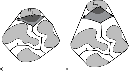
Figure 30. For $\Omega_{1}$ in configurations using convex hull bounding regions, measure of positional significance is the ratio of the volume of the darkest region to the volume of the union of the two more darkly shaded regions. In a) $\Omega_{1}$ is central, while in b) when $\Omega_{1}$ is moved away from the remaining regions, it becomes less significant for the configuration as indicated by the decreasing ratio.

Properties of Invariants for Closeness and Positional Significance

We consider three properties of these invariants:

• computation of all of the invariants as skeletal linking integrals;

• invariance under the action of the Euclidean group and scaling; and

• continuity of the invariants under small perturbations of generic configurations.

Computation of the Invariants as Skeletal Linking Integrals

We can use the results from the previous section to compute as skeletal linking integrals the above volumes of regions associated to $\boldsymbol{\Omega}$. This is summarized by the following.

Theorem 11.3.

If $\boldsymbol{\Omega}=\{\Omega_{i}\}\subset\tilde{\Omega}$ is a multi-region configuration, with a skeletal linking structure, then all global invariants of the configuration which can be expressed as integrals over regions in ${\mathbb{R}}^{n+1}$ can be computed as skeletal linking integrals using Theorem 10.6. In particular, the invariants $c_{i\to j}$, $c_{i\,j}$, $c^{a}_{i\,j}$, and $s_{i}$ are given as the quotients of two skeletal linking integrals using (10.11) and (10.25).

$\Box$

Remark 11.4.

We could try to alternatively use boundary measures for the regions to define closeness and positional significance. There are two problems with this approach. From a computational point of view, the skeletal structures could only be used where the partial Blum condition is satisfied. Moreover, boundary measures do not capture how much of the regions are close to each other (only where their boundaries are close). For these reasons we have concentrated on (ratios of) volumetric measures to capture positional geometry of the configuration.

Invariance under the action of the Euclidean Group and Scaling

Second, we establish the invariance of the invariants defining closeness and positional significance under Euclidean motions and scaling. Let $\boldsymbol{\Omega}=\{\Omega_{i}\}\subset\tilde{\Omega}$ be a multi-region configuration, with a skeletal linking structure $\{(M_{i},U_{i},\ell_{i})\}$. If $f$ is a Euclidean motion and $a>0$ is a scaling factor, then we may let $\boldsymbol{\Omega}^{\prime}=\{\Omega_{i}^{\prime}\}\subset\tilde{\Omega}^{\prime}$, where $\Omega_{i}^{\prime}=f(\Omega_{i})$ and $\tilde{\Omega}^{\prime}=f(\tilde{\Omega})$. We also let $\{(M_{i}^{\prime},U_{i}^{\prime},\ell_{i}^{\prime})\}$ be a skeletal linking structure for $\boldsymbol{\Omega}^{\prime}$ defined by $M_{i}^{\prime}=f(M_{i})$, $U_{i}^{\prime}=f(U_{i})$, and $\ell_{i}^{\prime}=\ell_{i}$. As $f$ preserves distance and angles, we have $r_{i}^{\prime}=r_{i}$, and the image of the linking flow for $\boldsymbol{\Omega}$ is the linking flow for $\boldsymbol{\Omega}^{\prime}$. Then, $\{(M_{i}^{\prime},U_{i}^{\prime},\ell_{i}^{\prime})\}$ satisfies the conditions for being a skeletal linking structure for $\boldsymbol{\Omega}^{\prime}$. As $\tilde{\Omega}^{\prime}=f(\tilde{\Omega})$, the corresponding bounded linking structure for $\boldsymbol{\Omega}^{\prime}$ using $\tilde{\Omega}^{\prime}$ is the image of that for $\boldsymbol{\Omega}$ for $\tilde{\Omega}$. Then, the associated linking regions for $\boldsymbol{\Omega}^{\prime}$ are the images of the corresponding associated linking regons for $\boldsymbol{\Omega}$. Since $f$ preserves volumes, the invariants for closeness and positional significance are preserved by $f$.

If instead we consider a scaling by the factor $a>0$, then we let $g_{a}(x)=a\cdot x$. Now the images of $\boldsymbol{\Omega}$ and $\tilde{\Omega}$ under $g_{a}$ define a configuration $\boldsymbol{\Omega}^{\prime}$ in $\tilde{\Omega}^{\prime}$. We likewise let $\{(M_{i}^{\prime},U_{i}^{\prime},\ell_{i}^{\prime})\}$ be defined by $M_{i}^{\prime}=g_{a}(M_{i})$, $U_{i}^{\prime}=aU_{i}$, and $\ell_{i}^{\prime}=a\ell_{i}$ (and $r_{i}^{\prime}=ar_{i}$). As before this is a skeletal structure for $\boldsymbol{\Omega}^{\prime}$. Everything goes through except that $g_{a}$ multiplies volume by $a^{n+1}$. However, as the invariants are ratios of volumes, they again do not change. We summarize this with the following.

Proposition 11.5.

If $\boldsymbol{\Omega}=\{\Omega_{i}\}\subset\tilde{\Omega}$ is a multi-region configuration, with a skeletal linking structure, then $c_{i\to j}$, $c_{i\,j}$, $c^{a}_{i\,j}$, and $s_{i}$ are invariant under the action of a Euclidean motion and scaling applied to both $\boldsymbol{\Omega}$ and $\tilde{\Omega}$ for the image of the skeletal linking structure for the image configuration and bounding region.

$\Box$

We note that if we consider the absolute positional significance $\tilde{s}_{i}$, then it is still invariant under Euclidean motions. However, under scaling by $a>0$, it changes by the factor $a^{n+1}$; but this would not alter the hierarchy based on absolute positional significance, as all $\tilde{s}_{i}$ would be multiplied by the same factor.

Remark 11.6.

Importantly, the invariance in Proposition 11.5 crucially depends on also applying the Euclidean motion and/or scaling to the bounding region $\tilde{\Omega}$. If the region is either fixed, or depends upon an external condition which prevents it from transforming along with the configuration, then the invariance does not hold. This has important consequences when properties of the configuration are measured, and is a problem for many methods in imaging where the imaged region first has to be normalized in some way. In our case, the measurements should also be taking into account how their relation with the bounding region changes.

Continuity and Changes under Small Perturbations

Lastly, suppose that $\boldsymbol{\Omega}=\{\Omega_{i}\}\subset\tilde{\Omega}$ is a multi-region configuration, with a bounded skeletal linking structure. We ask how the invariants will change under small perturbations. This is a generally challenging question which we are not attempting to answer in this paper. Thus, for what we do say, we will not give precise proofs, but indicate what we expect to happen.

First, if the linking structure is a Blum linking structure, then only if the objects undergo a sufficiently small deformation for say the $C^{\infty}$ topology will there be the stability of the Blum linking structure, so the Blum medial axes will deform in a smooth fashion. Then, the associated regions will also deform in a piecewise smooth fashion. Hence, the volumes of these regions will vary continuously. Thus, the quotients of the volumes will also vary continuously. It then follows that the invariants, which are quotients of such volumes will also vary continuously.

If instead we only require that the deformations be $C^{1}$ small then the Blum linking structure will be unstable; however, it is possible to deform it to a skeletal linking structure which changes continuously under this small deformation. Under these changes the skeletal sets will deform without changing their basic structure, and the associated regions will change in a continuous fashion so the resulting invariants, which are volumetric based, will also change in a continuous fashion.

How exactly they will change will depend on the particular deformation and this will demand a precise analysis that we are not prepared to carry out here. However, as a simple example, suppose we enlarge one of the regions $\Omega_{i}$ by increasing the radial vectors by a factor $a>1$, so that $ar_{i}<\ell_{i}$, and without altering the remainder of the skeletal structure. If the region remains in the bounding region and doesn’t intersect itself or other regions, then the ratio ${\rm vol}\,(\Omega_{i\to j})$ to ${\rm vol}\,(\mathcal{R}_{i\to j})$ will increase for each $j$ so the $s_{i}$ will increase, as will the $c_{i\to j}$. If instead $0<a<1$, then $s_{i}$ and $c_{i\to j}$ will decrease.

If instead we move the region $\Omega_{i}$ in a direction away from all of the other regions without altering its size, then in general $s_{i}$ will decrease, and conversely if we move it toward the other regions, generally $s_{i}$ will increase. Thus, the invariants capture the type of geometric properties that we would hope.

Tiered Linking Graph

Now that we have obtained invariants appropriately measuring closeness and positional significance among objects, we can combine these into a graph theoretic structure. We define exactly the type of graph structure we consider. For us a graph $\Gamma$ is defined by a finite set of vertices $V=\{v_{i}:i=1,\dots,m\}$, and a set of unordered edges $E=\{e_{i\,j}\}$ with at most one edge $e_{i\,j}$ between any pair of distinct vertices $v_{i}$ and $v_{j}$.

Definition 11.7.

A tiered graph consists of a graph $\Gamma$ together with a discrete nonnegative function $f:V\cup E\to{\mathbb{R}}_{+}$ which we shall more simply denote by $f:\Gamma\to{\mathbb{R}}_{+}$. The discrete function $f$ has values $f(v_{i})=a_{i}\geq 0$ for each vertex $v_{i}$, and $f(e_{i\,j})=b_{i\,j}\geq 0$ for each edge $e_{i\,j}$.

Given such a tiered graph, we can view its values on vertices and edges as height functions assigning weights to the vertices and edges; and then apply “thresholds”to $f$ to identify subgraphs, consisting of distinguished vertices and edges. First, given a value $b>0$, we can consider the subgraph $\Gamma_{b}$ consisting of all vertices, but only those edges where $f\geq b$. $\Gamma_{b}$ decomposes into connected subgraphs consisting of vertices which have edges of weights $>b$. As $b$ decreases from $B=\max\{b_{i\,j}\}$, then we see the smaller graphs begin to merge as edges are added, until we reach $\Gamma$ for $b=\min\{b_{i\,j}\}$. In fact, as pointed out by the referee this approach is similar to the known method of “clustering”for collections of points.

If instead we consider the threshold $a$ for $f$ on vertices, then instead we define $\Gamma^{a}$ to consist of those vertices with $f\geq a$, and only those edges joining two vertices within this set. This identifies a subgraph consisting of the most important vertices as measured by weights, along with the edges between these vertices. Then as $a$ decreases from $A=\max\{a_{i}\}$, we again see the small graphs being supplemented by additional vertices with edges being added from these vertices until we reach the full graph when $a=\min\{a_{i}\}$. This gives a hierarchical structure to the graph $\Gamma$. Along with the subgraphs and the hierarchical structure, we can also identify vertices which are joined by strongly weighted edges, and important vertices with large weights $a_{i}$, and less significant ones with small weights $a_{i}$. It would also be possible to use this to turn $\Gamma$ into a directed graph where the direction of an edge is from lower positional significance to one of higher.

Figure 31. Example of a tiered graph structure which we view as lying in a horizontal plane with one horizontal axis indicating positional significance, and the values of the height function giving values $c$ on the edges indicated by the heights of the dotted lines above the edges.

This approach, using the tiered graph structure, applies to a configuration of multi-regions with a skeletal linking structure. We define the associated tiered linking graph $\Lambda$ as follows. For each region $\Omega_{i}$, we assign a vertex $v_{i}$ in $\Lambda$, and to each pair of neighboring regions $\Omega_{i}$ and $\Omega_{j}$, we assign an edge $e_{i\,j}$ joining the corresponding vertices. If the regions are not neighbors, there is no edge. We define the height function $f$ by: $f(v_{i})=s_{i}$ and $f(e_{i\,j})=c_{i\,j}$ (or $c^{a}_{i\,j}$).

An example is shown in Figure 31. Then, when we apply the thresholds, we remove vertices to the left of some vertical line or edges whose heights are below some height. We see how subconfigurations associated to the subgraphs merge into larger configurations as the vertical line indicating $s$ moves to the left, or the height moves downwards, with the resulting graphs based on closeness of the regions or their positional significance. Also, the position along the $s$-axis identifies the hierarchy of regions in the configuration.

Remark 11.8.

Although we have used the term “threshold”  here to identify graph theoretic features, this differs considerably from the notion of threshold $\tau$ that we referred to in §9 when we discussed the bounding region, and how the threshold $\tau$ would introduce a parametrized family of invariants that would offer more detailed information about the positional geometry of the configuration. The height function that we have defined here would become a parametrized family of height functions depending on $\tau$.

Higher Order Positional Geometric Relations via Indirect Linking

We conclude this introduction to positional geometry by observing that the skeletal linking structures we have introduced only relate neighboring regions. We have shown that the skeletal linking structures (and specifically the full Blum medial linking structures) capture both the shape properties of individual regions (and their geometry), and the geometry of the external region yielding positional information. However, this approach allows regions to hide other regions from the geometric influence of non-neighbors. One way to overcome this is to work with “indirect linking”  where two regions are linked via a third region $\Omega_{3}$. For example, if we add a small elliptical region $\Omega_{4}$ to the configuration in a) of Figure 32, we obtain b) of the figure. The small region alters the closeness of regions $\Omega_{1}$ and $\Omega_{2}$. However, we see in b) that the linking neighborhood for the $\Omega_{4}$ lies in the linking region between $\Omega_{1}$ and $\Omega_{2}$ in a). Hence, if we allowed indirect linking through $\Omega_{4}$, then the closeness of $\Omega_{1}$ and $\Omega_{2}$ would not be altered. This is just one example of various aspects of configurations that could be better understood by deriving indirect linking properties from the linking structure. While the numerical measures could not be deduced just using the values from linking, the occurence of indirect linking could already be seen from the tiered graph structure. However, we will not attempt to develop this further in this paper.

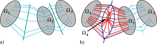
Figure 32. Indirect linking when a region $\Omega_{4}$ is added between regions in a) yielding b). The Blum linking structure in b) has the neighborhood of $\Omega_{4}$ contained in the neighboring regions of $\Omega_{1}$ and $\Omega_{2}$, so if indirect linking through $\Omega_{4}$ is allowed, then there is no change in the closeness of $\Omega_{1}$ and $\Omega_{2}$.

12. Multi-Distance and Height-Distance Functions and Partial Multi-Jet Spaces

In order to prove the existence of a medial linking structure for a generic multi-region configuration it will be necessary to prove a generalization of the transversality theorem used by Mather [M1] for the case of single regions. This version will be applied in several different forms to a configuration $\boldsymbol{\Omega}=\{\Omega_{i}\}$ in ${\mathbb{R}}^{n+1}$, via a model configuration $\boldsymbol{\Delta}=\{\Delta_{i}\}$ and embedding $\Phi:\boldsymbol{\Delta}\to{\mathbb{R}}^{n+1}$ as in §2.

For such a configuration, we will consider a collection of functions including: “distance functions”, “height functions”, “multi-distance functions”, and “height-distance functions”. The transversality theorem applied to each one will yield for each compact set containing the configuration in its interior a residual set of embeddings $\Phi$ such that appropriate genericity properties hold. Then, we use the special properties of the regions and the functions to see that the set of such embeddings is actually open. Hence, the set of generic embeddings will be open and dense.

Multi-Distance and Height-Distance Functions

For a multi-region configuration given by an embedding $\Phi:\boldsymbol{\Delta}\to{\mathbb{R}}^{n+1}$, we define the associated multi-distance and height-distance functions. However, we change the emphasis (and notation) from that of functions defined on subsets of the ambient space ${\mathbb{R}}^{n+1}$ to functions defined via the embedding $\Phi$ on the model configuration $\boldsymbol{\Delta}$.

Stratification of the Configuration

For $\boldsymbol{\Delta}$ we introduce notation to keep track of various strata of the boundaries of each $\Delta_{i}$ and their corresponding images $\Omega_{i}$ under $\Phi$. As in §2, the boundary of $\Delta_{i}$ is denoted by $X_{i}$; and we let $X=\cup_{i}X_{i}$ denote the stratified set which is the union of the boundaries. We also let $X_{ij}$ denote the union of the smooth strata of $X_{i}\cap X_{j}$ (i.e. those of dimension $n$). We also let for each $i>0$, $X_{i0}=X_{i}\backslash(\cup_{j>0}Cl(X_{ij}))$. For regions satisfying the boundary edge condition, $\Delta_{i}\cap\Delta_{j}=Cl(X_{ij})$; thus, $X_{i0}$ is an open stratum of $X_{i}$ and the points of $X_{i0}$ do not lie in any region other than $X_{i}$. For the configuration $\boldsymbol{\Omega}$, with complement $\Omega_{0}$, the smooth strata consist of the image of the union $\cup_{i}X_{i\,0}$. Just as for $X_{i\,j}$, we let $X_{0\,i}=X_{i\,0}$ to emphasize that the image of $X_{0\,i}$ is a smooth stratum of $\Omega_{0}$. Lastly, the remaining strata are formed from the $k$-edge-corner points for each given $k$.

For any $\Delta_{i}$, we define an index set $\mathcal{J}_{i}=\{j\neq i:X_{ij}\neq\emptyset\}$. For $i=0$, we let $\mathcal{J}_{0}=\{j>0:X_{0j}\neq\emptyset\}$. Also, for $i\geq 0$ we let $q_{i}=|\mathcal{J}_{i}|$. For each $i\geq 0$ we let $\stackrel{{\scriptstyle\circ}}{{X}}_{i}=\coprod_{j\in\mathcal{J}_{i}}X_{ij}$, which is the set of points in smooth strata of $X_{i}$. Next, we let $X_{\mathcal{J}_{i}}=\coprod_{j\in\mathcal{J}_{i}}\stackrel{{\scriptstyle\circ}}{{X}}_{j}$, which is the disjoint union of the smooth strata of those $X_{j}$ for which $X_{i\,j}\neq\emptyset$ (i.e. are adjoined to $X_{i}$). We note that each point in $\stackrel{{\scriptstyle\circ}}{{X}}_{i}$ belongs to exactly one of the components of $X_{\mathcal{J}_{i}}$; however if there are $j,j^{\prime}\in\mathcal{J}_{i}$ with $X_{j\,j^{\prime}}\neq\emptyset$, then any point $x\in X_{j\,j^{\prime}}$ has representatives which belong to both $\stackrel{{\scriptstyle\circ}}{{X}}_{j}$ and $\stackrel{{\scriptstyle\circ}}{{X}}_{j^{\prime}}$.

This is the space on which the models for “simple linking”will be defined. However, to model both partial and self-linking, we must allow multiple copies of some of the $\stackrel{{\scriptstyle\circ}}{{X}}_{j}$. We do so by extending the above definition using an assignment function. Given $m>0$, we consider an assignment, which is a discrete function for integers $1\leq p\leq m$, sending $p\mapsto j_{p}\in\mathcal{J}_{i}$. Then, with this assignment, we define $X_{\mathcal{J}_{i}}=\coprod_{p=1}^{m}\stackrel{{\scriptstyle\circ}}{{X}}_{j_{p}}$. Note that because of the complexity of the notation which we will need to introduce, we do not include the assignment in the notation for $X_{\mathcal{J}_{i}}$ but will instead refer specifically to the assignment used for defining $X_{\mathcal{J}_{i}}$. The basic model above for $X_{\mathcal{J}_{i}}$ uses the assignment for $m=q_{i}$ bijectively mapping $\{p\in{\mathbb{Z}}:1\leq p\leq q_{i}\}$ to $\mathcal{J}_{i}$.

Example 12.1 illustrates $X_{\mathcal{J}_{i}}$ for a multi-region configuration given in Figure 33. We will let the images of these subspaces of the $X_{i}$ under $\Phi$ inherit the same notation, e.g. $\Phi(X_{i\,0})=\mathcal{B}_{i\,0}$, etc.

We will also use the notation $\Sigma_{Q\,i}\subset X_{i}$ to denote the stratification by smooth $Q_{k}$-points in $X_{i}$. Then, we note that while $\stackrel{{\scriptstyle\circ}}{{X}}_{i}$ consists of points in the smooth strata, $\stackrel{{\scriptstyle\circ}}{{X}}_{i}\cap\Sigma_{Q\,i}=\emptyset$, and the points in $\Sigma_{Q\,i}$ are also smooth points on the boundary $X_{i}$.

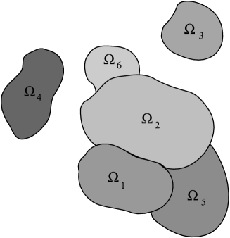
Figure 33. A multi-region configuration in ${\mathbb{R}}^{2}$ given earlier with the decomposition explained in Example 12.1.

Example 12.1.

In Figure 33 is a multi-region configuration $\boldsymbol{\Omega}$ defined by the model $\Phi:\boldsymbol{\Delta}\to{\mathbb{R}}^{n+1}$. We describe the properties of the image regions $\{\Omega_{i}\}$ in terms of the model $\boldsymbol{\Delta}$. Both $X_{3}=\partial\Delta_{3}$ and $X_{4}=\partial\Delta_{4}$ are smooth so $\mathcal{J}_{3}=\mathcal{J}_{4}=\{0\}$. However, for $\Delta_{2}$, $\mathcal{J}_{2}=\{0,1,5,6\}$ and for $\Delta_{1}$, $\mathcal{J}_{1}=\{0,2,5\}$. For each $i=1,2,5,6$, $X_{\mathcal{J}_{i}}$ without repetitions consists of disjoint unions of smooth boundary curves of those regions $\Delta_{j}$ which share a portion of their boundary with $\Delta_{i}$. The images of these curves give the corresponding curves of shared boundary regions between $\Omega_{j}$ and $\Omega_{i}$. For example, the regions $\Omega_{1}$, $\Omega_{5}$, $\Omega_{6}$ are adjoined to $\Omega_{2}$ along the boundary curves which are images of $X_{21}$; $X_{25}$, and $X_{26}$. All regions are adjoined to the complement.

Our future computations shall concern transversality conditions on mappings associated to $\Phi\in{\rm Emb}\,(\boldsymbol{\Delta},{\mathbb{R}}^{n+1})$. For this reason we shall reintroduce the distance and height functions so they are defined on $X$. The distance function on $X$ via the embedding $\Phi$ is the function $\sigma:X\times{\mathbb{R}}^{n+1}\to{\mathbb{R}}$ defined by $\sigma(x,u)=\|\Phi(x)-u\|^{2}$. Likewise, the height function via the embedding $\Phi$ is the function $\nu:X\times S^{n}\to{\mathbb{R}}$ defined by $\nu(x,v)=\langle\Phi(x),v\rangle$, where $S^{n}$ is the unit sphere in ${\mathbb{R}}^{n+1}$. Using these basic functions we define both multi-distance functions and height-distance functions.

We also introduce a variant form of the distance function for regions with singular boundaries to allow it to be defined at the nonsingular $Q_{k}$ points. We let $X_{i}^{*}$ denote the set of smooth points of $X_{i}$ obtained by removing the points of type $P_{k}$ and singular $Q_{k}$ points, for all $k$. We note that $\Sigma_{Q\,i}\subset X_{i}^{*}$, and that $X_{i}^{*}$ differs from the set $\stackrel{{\scriptstyle\circ}}{{X}}_{i}$ by including the nonsingular $Q_{k}$ points of $X_{i}$. Then we define the distance function $\sigma_{i}=\sigma|(X_{i}^{*}\times{\mathbb{R}}^{n+1})$. In addition to obtaining the generic properties of the distance function, we shall also see that it generically satisfies transversality conditions relative to the strata of $\Sigma_{Q\,i}$.

We will use the standard notation that $Y^{r}=Y\times\cdots\times Y$ ($r$ factors), and let $\Delta^{(r)}Y\subset Y^{r}$ be the generalized diagonal consisting of $(y_{1},\cdots,y_{r})\in Y^{r}$ such that $y_{i}=y_{j}$ for some $i\neq j$. We also let $\Delta^{r}Y\subset Y^{r}$ denote the exact diagonal consisting of $(y,\cdots,y)\in Y^{r}$. Then, we let $Y^{(r)}\overset{def}{=}Y^{r}\backslash\Delta^{(r)}Y$.

For each $j=0,1,\dots,m$, we let ${\mathbb{R}}^{n+1}_{j}$ denote a copy of ${\mathbb{R}}^{n+1}$ indexed by $j$, and we abbreviate $\prod_{j=0}^{m}{\mathbb{R}}^{n+1}_{j}=({\mathbb{R}}^{n+1})^{m+1}$. Then $({\mathbb{R}}^{n+1})^{(m+1)}$ denotes the complement of the generalized diagonal in $({\mathbb{R}}^{n+1})^{m+1}$. Quite generally we let $\pi_{j}:\prod_{i=0}^{k}{\mathbb{R}}^{n+1}_{i}\to{\mathbb{R}}^{n+1}_{j}$ denote both the projection on the $j$–th factor, as well as its restriction to $({\mathbb{R}}^{n+1})^{(k+1)}\subset\prod_{i=0}^{k}{\mathbb{R}}^{n+1}_{i}$.

Given an assignment for $1\leq p\leq m$, $p\mapsto j_{p}\in\mathcal{J}_{i}$. We denote points in $({\mathbb{R}}^{n+1})^{(m)}$ by $(u^{(j_{1})},\dots,u^{j_{(m)}})$, where we let $u^{(j_{p})}$ have coordinates $(u^{(j_{p})}_{1},\dots,u^{(j_{p})}_{n+1})$. This will allow us to consider multiple centers $u^{(j_{p})}$ for distance functions on boundaries of given regions $\stackrel{{\scriptstyle\circ}}{{X}}_{j}$ with $j=j_{p}$.

Definition 12.2.

A multi-distance function associated to the $i$-th region $\Omega_{i}$ for the configuration $\boldsymbol{\Omega}$ defined by the model $\Phi:\boldsymbol{\Delta}\to{\mathbb{R}}^{n+1}$, together with $m>0$ and an assignment $p\mapsto j_{p}$, is given by

(12.1) $$\rho_{i}:X_{\mathcal{J}_{i}}\times({\mathbb{R}}^{n+1})^{(m+1)} \rightarrow{\mathbb{R}}^{2},$$

$$(x,(u^{(j_{1})},\dots,u^{(j_{m})},u^{(i)})) \mapsto(\sigma(x,u^{(i)}),\sigma(x,u^{(j_{p})}))\quad\makebox{ for }x\in\stackrel{{\scriptstyle\circ}}{{X}}_{j_{p}}\,.$$

These functions are “multi-distance”  functions in the sense that they incorporate multiple functions capturing the squared distance from distinct points $u^{(j)}$ in the ambient space, and ultimately we are interested in the case where the $u^{(q)}\in{\rm int}\,(\Omega_{j})$ for $j\in\mathcal{J}_{i}$.

Next we define height-distance functions associated to each region $\Delta_{i}$.

Definition 12.3.

The height-distance function associated to the configuration $\boldsymbol{\Omega}$ defined by the model $\Phi:\boldsymbol{\Delta}\to{\mathbb{R}}^{n+1}$ together with $m>0$ and an assignment $p\mapsto j_{p}$ and is given by

(12.2) $$\tau:X_{\mathcal{J}_{0}}\times({\mathbb{R}}^{n+1})^{(m)}\times S^{n} \rightarrow{\mathbb{R}}^{2},$$

$$(x,(u^{(j_{1})},\dots,u^{(j_{m})}),v) \mapsto(\nu(x,v),\sigma(x,u^{(j_{p})}))\quad\makebox{ for }x\in\stackrel{{\scriptstyle\circ}}{{X}}_{j_{p}}$$

where $\mathcal{J}_{0}=\{j:X_{0,j}\neq\emptyset\}$

Notation: In what follows, we shall frequently abbreviate $\sigma(x,u^{(j)})$ as $\sigma_{j}(x)$.

The height-distance function will be used to relate the distance squared functions for different points $u^{(j)}$ in the ambient space and properties of the height function on $X_{\mathcal{J}_{0}}$. We shall apply a transversality theorem to these two families of multi-functions for various $m$ and assignments $p\mapsto j_{p}$ to deduce the genericity of properties of linking (in the case of $\rho_{0}$) and those relating linking with the boundary of the unlinked region. Since the transversality theorem is a result on the level of jet bundles, our focus in the next section is on defining a special type of “partial multijet space”  and a special kind of multijets of such functions which map into these spaces.

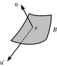
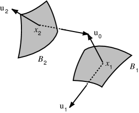
(a)                                              (b)

Figure 34. a) Multi-distance function - pair of families of distance functions from a region boundary to distinct points $u$ and $u^{\prime}$ in the complement. b) Linking via multi-distance functions - families of distance functions from region boundaries $\mathcal{B}_{i}$ to a common point $u_{0}$ in the complement.

Partial Jet Spaces for Multi-Distance and Height-Distance Functions

To examine the generic properties of linking between regions, we introduce the partial multijet space and the corresponding partial multijet extension maps for both multi-distance and height-distance functions.

Given an integer $s>0$, $i$, an integer $m>0$ with assignment $p\mapsto j_{p}$, we let $\mathbf{\ell}=(\ell_{1},\dots,\ell_{q_{i}})$ denote an ordered partition of the form $s=\ell_{1}+\cdots+\ell_{m}$ with each integer $\ell_{p}>0$. For each $1\leq p\leq m$, we denote points $x^{(j_{p})}=(x^{(j_{p})}_{1},\dots,x^{(j_{p})}_{\ell_{p}})\in\stackrel{{\scriptstyle\circ}}{{X}}_{j_{p}}^{(\ell_{p})}$. Define

(12.3) $$X_{\mathcal{J}_{i}}^{(\mathbf{\ell})}\,\, =\,\,\{(x^{(j_{1})},\dots,x^{(j_{m})})\in\stackrel{{\scriptstyle\circ}}{{X}}_{j_{1}}^{(\ell_{1})}\times\cdots\times\stackrel{{\scriptstyle\circ}}{{X}}_{j_{m}}^{(\ell_{m})}:x_{1}^{(j_{p})}\in X_{i\,j_{p}}\text{ for all $p$ and }$$

$$\qquad\qquad\text{ if }j_{p}=j_{p^{\prime}},\text{then }x_{q}^{(j_{p})}\neq x_{q^{\prime}}^{(j_{p^{\prime}})}\text{for any }q,q^{\prime}\}\,.$$

Observe that $X_{\mathcal{J}_{i}}^{(\mathbf{\ell})}$ is an open subset of the product space in (12.3). We denote a point in $X_{\mathcal{J}_{i}}^{(\mathbf{\ell})}$ by $(x^{(j_{1})},\dots,x^{(j_{m})})$, where each $x^{(j_{p})}=(x^{(j_{p})}_{1},\dots,x^{(j_{p})}_{\ell_{p}})$. By definition, for any $s$-tuple in $X_{\mathcal{J}_{i}}^{(\mathbf{\ell})}$, any two points in it belonging to the same $\stackrel{{\scriptstyle\circ}}{{X}}_{j}$ are distinct. However, we still note that not every $s$-tuple need belong to $X^{(s)}$. This is because if there are $j_{p}\neq j_{p^{\prime}}$ with $X_{j_{p}\,j_{p^{\prime}}}\neq\emptyset$, then any point $x\in X_{j_{p}\,j_{p^{\prime}}}$ is represented in the disjoint copies of both $\stackrel{{\scriptstyle\circ}}{{X}}_{j_{p}}$ and $\stackrel{{\scriptstyle\circ}}{{X}}_{j_{p^{\prime}}}$. Nonetheless the multi-function $\rho_{i}$ will be defined for $x\in\stackrel{{\scriptstyle\circ}}{{X}}_{j}$ by $(\sigma(x,u^{(i)}),\sigma(x,u^{(j_{p})}))$ versus for $x\in\stackrel{{\scriptstyle\circ}}{{X}}_{j_{p^{\prime}}}$, by $(\sigma(x,u^{(i)}),\sigma(x,u^{(j_{p^{\prime})}}))$, with $u^{(j_{p})}\neq u^{(j_{p^{\prime}})}$. A consequence is that the transversality conditions on $\stackrel{{\scriptstyle\circ}}{{X}}_{j_{p}}$ and $\stackrel{{\scriptstyle\circ}}{{X}}_{j_{p^{\prime}}}$ are different and will be verified independently. This motivates our definition of the partial multijet spaces to follow.

We consider the usual $k$-multijet space ${{}_{s}}J^{k}(X,{\mathbb{R}}^{2})$, which consists of $s$ $k$-jets of germs at distinct points of $X$ mapping to ${\mathbb{R}}^{2}$, and we define a subspace using the partition $\mathbf{\ell}$.

Definition 12.4.

For $X_{\mathcal{J}_{i}}$ (defined for $m>0$ with an assignment $p\mapsto j_{p}$, let $\mathbf{\ell}=(\ell_{1},\dots,\ell_{m})$ be an ordered partition of $s>0$. Then, the partial $\mathbf{\ell}$-multi $k$-jet space is the subspace of ${{}_{s}}J^{k}(X_{\mathcal{J}_{i}},{\mathbb{R}}^{2})$ defined by the restriction

(12.4) $${{}_{\mathbf{\ell}}}E^{(k)}(X_{\mathcal{J}_{i}},{\mathbb{R}}^{2})\,\,=\,\,\left(\prod_{p=1}^{m}\,{{}_{\ell_{p}}}J^{k}(\stackrel{{\scriptstyle\circ}}{{X}}_{j_{p}},{\mathbb{R}}^{2})\right)|\,(X_{\mathcal{J}_{i}})^{(\ell)}.$$

The two basic properties of multijet spaces which are shared by the partial multijet spaces are summarized in the following straightforward lemma.

Lemma 12.5.

The partial multijet spaces have the following properties:

• ${{}_{\mathbf{\ell}}}E^{(k)}(X_{\mathcal{J}_{i}},{\mathbb{R}}^{2})$ is a smooth submanifold of ${{}_{s}}J^{k}(X_{\mathcal{J}_{i}},{\mathbb{R}}^{2})$; and

• ${{}_{\mathbf{\ell}}}E^{(k)}(X_{\mathcal{J}_{i}},{\mathbb{R}}^{2})$ is a locally trivial fiber bundle over $X_{\mathcal{J}_{i}}^{(\mathbf{\ell})}$ with fiber

  $\prod_{p=1}^{m}\,(J^{k}(n,2)\times{\mathbb{R}}^{2})^{\ell_{p}}$.

$\Box$

Both the multi-distance and height-distance functions defined for $m>0$ with an assignment $p\mapsto j_{p}\in\mathcal{J}_{i}$, are given as mappings of the form $\psi:X_{\mathcal{J}_{i}}\times U\to{\mathbb{R}}^{2}$, where $U$ is either $({\mathbb{R}}^{n+1})^{(m+1)}$ or $({\mathbb{R}}^{n+1})^{(m)}\times S^{n}$. For such mappings we define an associated partial multijet map

$$_{\mathbf{\ell}}j^{k}(\psi): \,X_{\mathcal{J}_{i}}^{(\mathbf{\ell})}\times U\longrightarrow\,{{}_{\mathbf{\ell}}}E^{(k)}(X_{\mathcal{J}_{i}},{\mathbb{R}}^{2})$$

(12.5) $$((x^{(j_{1})},\cdots,x^{(j_{m})}), u)\mapsto({{}_{\ell_{1}}}j_{1}^{k}(\psi(x^{(j_{1})},u),\dots,{{}_{\ell_{m}}}j_{1}^{k}(\psi(x^{(j_{m})},u)))$$

where ${}_{\ell_{p}}j_{1}^{k}(\psi(x^{(j_{p})},u))$ denotes the multijet ${}_{\ell_{p}}j^{k}(f)$ for the function $f=\psi(\cdot,u)$ (for a fixed $u$) on $\stackrel{{\scriptstyle\circ}}{{X}}_{j_{p}}$. In the special cases of the multi-distance and height-distance functions we obtain partial multijet maps

(12.6) $$_{\mathbf{\ell}}j^{k}(\rho_{i}):\,X_{\mathcal{J}_{i}}^{(\mathbf{\ell})}\times({\mathbb{R}}^{n+1})^{(m+1)}\longrightarrow\,{{}_{\mathbf{\ell}}}E^{(k)}(X_{\mathcal{J}_{i}},{\mathbb{R}}^{2})$$

and

(12.7) $$_{\mathbf{\ell}}j^{k}(\tau):\,X_{\mathcal{J}_{0}}^{(\mathbf{\ell})}\times({\mathbb{R}}^{n+1})^{(m)}\times S^{n}\longrightarrow\,{{}_{\mathbf{\ell}}}E^{(k)}(X_{\mathcal{J}_{0}},{\mathbb{R}}^{2})\,.$$

13. Generic Blum Linking Properties via Transversality Theorems

In this section, we state a transversality theorem for the multi-distance and height-distance functions associated to a multi-region configuration. We then list the submanifolds of partial multijet spaces which capture the generic linking properties. These are the submanifolds to which it will be applied.

Transversality Theorem for Multi-Distance and Height-Distance Functions

We begin with a variant of the transversality theorem of Looijenga for the distance functions for multi-region configurations defined by $\Phi:\boldsymbol{\Delta}\to{\mathbb{R}}^{n+1}$. The first transversality theorem concerns submanifolds of the $s$-multijet space that are ${}_{s}\mathcal{R}^{+}$-invariant. By this we mean that there is the induced action of the right equivalence group ${}_{s}\mathcal{R}$, via the action of $\mathcal{R}$ on $s$ multigerms, and we extend this by the group ${\mathbb{R}}$ acting by diagonal translations on ${\mathbb{R}}^{2}$, $(y_{1},y_{2})\mapsto(y_{1}+c,y_{2}+c)$ for $c\in{\mathbb{R}}$.

For later reference to the transversality theorems in [D5], we refer to the compact–open (or weak) $C^{\infty}$–topology as the regular $C^{\infty}$–topology. Since the underlying space of $\boldsymbol{\Delta}$ is compact, the Whitney and regular $C^{\infty}$ topologies on $C^{\infty}(\boldsymbol{\Delta},{\mathbb{R}}^{n+1})$ will agree.

Theorem 13.1.

For any $i=1,\dots,m$, let $W$ be a closed Whitney stratified subset of ${{}_{s}}J^{k}(X_{i}^{*},{\mathbb{R}})$ that is ${{}_{s}}\mathcal{R}^{+}$-invariant.

($a_{0}$) Let $Z\subset(X_{i}^{*})^{(s)}\times{\mathbb{R}}^{n+1}$ be compact. Then the set

$$\mathcal{W}\,\, =\,\,\{\Phi\in C^{\infty}(\boldsymbol{\Delta},{\mathbb{R}}^{n+1}):\text{ both }{{}_{s}}j_{1}^{k}\sigma_{i}\text{ and }{{}_{s}}j_{1}^{k}\sigma_{i}|((\Sigma_{Q})^{(s)}\times{\mathbb{R}}^{n+1})\,\,$$

$$\hskip 72.26999pt\overline{\pitchfork}\,\,W\subset{{}_{s}}J^{k}(X_{i}^{*},{\mathbb{R}})\text{ on Z}\}$$

is an open dense subset for the regular $C^{\infty}$–topology.

($b_{0}$) The set

$$\mathcal{W}\,\, =\,\,\{\Phi\in C^{\infty}(\boldsymbol{\Delta},{\mathbb{R}}^{n+1}):\text{ both }{{}_{s}}j_{1}^{k}\sigma_{i}\text{ and }{{}_{s}}j_{1}^{k}\sigma_{i}|((\Sigma_{Q})^{(s)}\times{\mathbb{R}}^{n+1})\,\,$$

$$\hskip 72.26999pt\overline{\pitchfork}\,\,W\subset{{}_{s}}J^{k}(X_{i}^{*},{\mathbb{R}})\text{ on }(X_{i}^{*})^{(s)}\times{\mathbb{R}}^{n+1}\}$$

is a residual subset for the regular $C^{\infty}$–topology.

Note: “$\overline{\pitchfork}$”  denotes transversality of the mapping to the strata of the Whitney stratified set.

Next, we give a multi-transversality theorem for the multi-distance and height-distance functions. Although we are principally interested in them for the multi-distance function $\rho_{0}$ to capture the generic linking properties, the proof is valid for any region $\Omega_{i}$ and yields a corresponding relation between a region $\Omega_{i}$ and its adjoining regions. For any smooth mapping $\Phi:\boldsymbol{\Delta}\to{\mathbb{R}}^{n+1}$ we obtain for any $i$, any integer $m>0$ with an assignment $p\mapsto j_{p}$, and a partition $\mathbf{\ell}=(\ell_{1},\dots,\ell_{m})$, the partial multijet mappings (12.6) and (12.7). The transversality theorem concerns these two mappings for a class of ${}_{\mathbf{\ell}}\mathcal{R}^{+}$-invariant distinguished submanifolds of the partial multijet space ${}_{\mathbf{\ell}}E^{(k)}(X_{\mathcal{J}_{i}},{\mathbb{R}}^{2})$ (see Definition 13.4). The ${}_{\mathbf{\ell}}\mathcal{R}^{+}$-action is the induced action of the right equivalence group ${}_{\mathbf{\ell}}\mathcal{R}$ on the fibers, extended by the diagonal action of ${\mathbb{R}}$ by translations on ${\mathbb{R}}^{2}$.

Theorem 13.2.

Let $\boldsymbol{\Delta}$ be a model for a multi-region configuration. Then, for any $i$, an $m>0$ with assignment $p\mapsto j_{p}$, and partition $\mathbf{\ell}=(\ell_{1},\dots,\ell_{q_{i}})$, let $W$ be a closed Whitney stratified subset of ${}_{\mathbf{\ell}}E^{(k)}(X_{\mathcal{J}_{i}},{\mathbb{R}}^{2})$ whose strata are ${}_{\mathbf{\ell}}\mathcal{R}^{+}$–invariant distinguished submanifolds (in the sense of Definition 13.4).

($a_{1}$) Let $Z\subset X_{\mathcal{J}_{i}}^{(\mathbf{\ell})}\times({\mathbb{R}}^{n+1})^{(m+1)}$ be compact. Then, the set

$$\mathcal{W}\,\,=\,\,\{\Phi\in C^{\infty}(\boldsymbol{\Delta},{\mathbb{R}}^{n+1}):{{}_{\mathbf{\ell}}}j_{1}^{k}\rho_{i}\;\overline{\pitchfork}\text{ on Z to }W\subset{{}_{\mathbf{\ell}}}E^{(k)}(X_{\mathcal{J}_{i}},{\mathbb{R}}^{2})\}$$

is an open dense subset for the regular $C^{\infty}$–topology.

($a_{2}$) Let $Z\subset X_{\mathcal{J}_{0}}^{(\mathbf{\ell})}\times({\mathbb{R}}^{n+1})^{(m)}\times S^{n}$ be compact. Then the set

$$\mathcal{W}^{\prime}\,\,=\,\,\{\Phi\in C^{\infty}(\boldsymbol{\Delta},{\mathbb{R}}^{n+1}):{{}_{\mathbf{\ell}}}j_{1}^{k}\tau\;\overline{\pitchfork}\text{ on Z to }W\subset{{}_{\mathbf{\ell}}}E^{(k)}(X_{\mathcal{J}_{0}},{\mathbb{R}}^{2})\}$$

is an open dense subset for the regular $C^{\infty}$–topology.

($b$) Both of the sets

$$\mathcal{W}\,\,=\,\,\{\Phi\in C^{\infty}(\boldsymbol{\Delta},{\mathbb{R}}^{n+1}):{{}_{\mathbf{\ell}}}j_{1}^{k}\rho_{i}\;\overline{\pitchfork}\,W\subset{{}_{\mathbf{\ell}}}E^{(k)}(X_{\mathcal{J}_{i}},{\mathbb{R}}^{2})\text{ on }X_{\mathcal{J}_{i}}^{(\mathbf{\ell})}\times({\mathbb{R}}^{n+1})^{(m+1)}\}$$

and

$$\mathcal{W}\,\,=\,\,\{\Phi\in C^{\infty}(\boldsymbol{\Delta},{\mathbb{R}}^{n+1}):{{}_{\mathbf{\ell}}}j_{1}^{k}\tau\;\overline{\pitchfork}\,W\subset{{}_{\mathbf{\ell}}}E^{(k)}(X_{\mathcal{J}_{0}},{\mathbb{R}}^{2})\text{ on }X_{\mathcal{J}_{0}}^{(\mathbf{\ell})}\times({\mathbb{R}}^{n+1})^{(m)}\times S^{n}\}$$

are residual subsets for the regular $C^{\infty}$–topology.

Note that in Theorems 13.1 and 13.2, $(b_{0})$ is a consequence of $(a_{0})$ and $(b)$ is a consequence of $(a_{1})$ and $(a_{2})$, for we may cover $X_{i}^{*}\times{\mathbb{R}}^{n+1}$, $X_{\mathcal{J}_{i}}^{(\mathbf{\ell})}\times({\mathbb{R}}^{n+1})^{(q_{i})}$ and $X_{\mathcal{J}_{0}}^{(\mathbf{\ell})}\times({\mathbb{R}}^{n+1})^{(q_{0})}\times S^{n}$ with countably many compact sets $C_{j}$ so that the sets in $(b_{0})$ and $(b)$ are countable intersections of open dense sets, hence residual. We will prove parts $(a_{0})$, $(a_{1})$ and $(a_{2})$ in §16 using a variant of the transversality theorems in [D5].

Remark 13.3.

These results give several types of extensions of the earlier transversality theorem due to Looijenga [L] and its extension due to Wall [Wa].

Submanifolds Defining Generic Properties of Blum Linking Structures

We next introduce the ${}_{\mathbf{\ell}}\mathcal{R}^{+}$-invariant distinguished submanifolds of the partial multijet space to which we will apply Theorem 13.2. This will yield the transversality results implying the generic linking conditions for configurations in the Blum case in ${\mathbb{R}}^{n+1}$ for $n\leq 6$.

We first introduce the general definition of the distinguished submanifolds which involves several classes of $\mathcal{R}$–invariant submanifolds of jet spaces and ${}_{\ell}\mathcal{R}^{+}$–invariant submanifolds of multijet spaces. These will include: both (an explicit list of) orbits of the $\mathcal{R}$ and ${}_{\ell}\mathcal{R}^{+}$ actions; their closures, which form Whitney stratified sets, together with the list of ${}_{\ell}\mathcal{R}^{+}$–invariant closed Whitney stratified subsets of higher codimension $>n+1$ which will be generically avoided.

General Form of the Class of Distinguished Submanifolds in ${}_{\mathbf{\ell}}E^{(k)}(X_{\mathcal{J}_{i}},{\mathbb{R}}^{2})$

For a given $i$ and $m>0$ with an assignment $p\mapsto j_{p}$ we let $\mathbf{\ell}=(\ell_{1},\ldots,\ell_{m})$ for integers $\ell_{p}>0$. We give the form of the distinguished submanifolds in ${}_{\mathbf{\ell}}E^{(k)}(X_{\mathcal{J}_{i}},{\mathbb{R}}^{2})$. By Lemma 12.5, ${{}_{\mathbf{\ell}}}E^{(k)}(X_{\mathcal{J}_{i}},{\mathbb{R}}^{2})$ is a locally trivial fiber bundle. For $S=(S_{1},\dots,S_{m})$ in $X_{\mathcal{J}_{i}}^{(\mathbf{\ell})}$ with $S_{p}\subset\stackrel{{\scriptstyle\circ}}{{X}}_{j_{p}}$ and $|S_{p}|=\ell_{p}$, the fiber at $S$ equals

(13.1) $$\prod_{p=1}^{m}{{}_{\ell_{p}}}J^{k}(\stackrel{{\scriptstyle\circ}}{{X}}_{j_{p}},{\mathbb{R}}^{2})_{S_{p}}\,\cong\,\prod_{p=1}^{m}\,(J^{k}(n,2)\times{\mathbb{R}}^{2})^{\ell_{p}}.$$

We let $W_{0\,p}$ denote ${}_{\ell_{p}}\mathcal{R}^{+}$ multi–orbits in the fibers ${}_{\ell_{p}}J^{k}(\stackrel{{\scriptstyle\circ}}{{X}}_{j_{p}},{\mathbb{R}})_{S_{p}}$ for $p=1,\dots,m$ (so in particular, in such a ${}_{\ell_{p}}\mathcal{R}^{+}$ multi–orbit the targets lie in $\boldsymbol{\Delta}^{\ell_{p}}{\mathbb{R}}$). As in the multijet case, the multi-orbits $W_{0\,p}$ in the fibers over points in $\stackrel{{\scriptstyle\circ}}{{X}}_{j_{p}}^{(\ell_{p})}$ fit together to form subbundles $W_{p}$ in ${{}_{\ell_{p}}}J^{k}(\stackrel{{\scriptstyle\circ}}{{X}}_{j_{p}},{\mathbb{R}})$ for $p=1,\dots,m$. Then

$$W_{1}\times\cdots\times W_{m}\,\,\subset\,\,\prod_{p=1}^{m}\,{{}_{\ell_{p}}}J^{k}(\stackrel{{\scriptstyle\circ}}{{X}}_{j_{p}},{\mathbb{R}})$$

restricts to a subbundle over $X_{\mathcal{J}_{i}}^{(\mathbf{\ell})}$.

For $p=1,\dots,m$, let $W^{\prime}_{p}$ denote a subbundle of $J^{k}(\stackrel{{\scriptstyle\circ}}{{X}}_{j_{p}},{\mathbb{R}})$ over $\stackrel{{\scriptstyle\circ}}{{X}}_{j_{p}}$ with fiber a $\mathcal{R}^{+}$–invariant submanifold. Typically it will denote either a $\mathcal{R}^{+}$–orbit for a $k$-jet of a germ, or a stratum of a Whitney stratification consisting of a union of orbits. We slightly abuse notation and define

(13.2) $$W^{\prime}\,\,=\,\,\prod_{p=1}^{m}(W^{\prime}_{p}\times(J^{k}(\stackrel{{\scriptstyle\circ}}{{X}}_{j_{p}},{\mathbb{R}}))^{\ell_{p}-1})\times\Delta^{m}{\mathbb{R}},$$

where for each $p$, $(W^{\prime}_{p})\times(J^{k}(\stackrel{{\scriptstyle\circ}}{{X}}_{j_{p}},{\mathbb{R}}))^{\ell_{p}-1})$ is restricted to lie over $\stackrel{{\scriptstyle\circ}}{{X}}_{j_{p}}^{(\ell_{p})}$ and the entries of $\Delta^{m}{\mathbb{R}}$ are in the first factor of each $(J^{k}(\stackrel{{\scriptstyle\circ}}{{X}}_{j_{p}},{\mathbb{R}}))^{\ell_{p}})$.

Therefore, $W^{\prime}\subset\prod_{p=1}^{m}\,{}_{\ell_{p}}J^{k}(\stackrel{{\scriptstyle\circ}}{{X}}_{j_{p}},{\mathbb{R}})$ restricts to a fiber bundle over $X_{\mathcal{J}_{i}}^{(\mathbf{\ell})}$, and

(13.3) $$W^{\prime}\times W_{1}\times\cdots\times W_{m}\,\,\subset\,\,\prod_{p=1}^{m}\,{{}_{\ell_{p}}}J^{k}(\stackrel{{\scriptstyle\circ}}{{X}}_{j_{p}},{\mathbb{R}})\times\prod_{p=1}^{m}\,{{}_{\ell_{p}}}J^{k}(\stackrel{{\scriptstyle\circ}}{{X}}_{j_{p}},{\mathbb{R}})$$

with the RHS restricting to the bundle ${{}_{\mathbf{\ell}}}J^{k}(X_{\mathcal{J}_{i}},{\mathbb{R}}^{2})$ over $(X_{\mathcal{J}_{i}})^{(\ell)}$.

Then we define

Definition 13.4.

Given $i$, $m>0$ with an assignment $p\mapsto j_{p}$, and the ordered partition $(\ell_{1},\dots,\ell_{m})$ with $s=\sum_{p=1}^{m}\ell_{p}$. Consider a collection of ${}_{\ell_{p}}\mathcal{R}^{+}$-invariant submanifolds $W_{p}\subset{{}_{\ell_{p}}}J^{k}(\stackrel{{\scriptstyle\circ}}{{X}}_{j_{p}},{\mathbb{R}})$ and $\mathcal{R}^{+}$-invariant submanifolds $W^{\prime}_{p}\subset J^{k}(\stackrel{{\scriptstyle\circ}}{{X}}_{j_{p}},{\mathbb{R}})$ for $p=1,\dots,m$, which each have the property that their closures are Whitney stratified sets for which they are open strata. Then, we form the subbundle of ${{}_{\mathbf{\ell}}}J^{k}(X_{\mathcal{J}_{i}},{\mathbb{R}}^{2})$ over $(X_{\mathcal{J}_{i}})^{\ell)}$ by the restriction of the LHS of (13.3). Any such subbundle will be called a distinguished submanifold in ${}_{\mathbf{\ell}}E^{(k)}(X_{\mathcal{J}_{i}},{\mathbb{R}}^{2})$.

Having defined such distinguished submanifolds, we next give the four classes of jet and multijet strata formed from $\mathcal{R}^{+}$ orbits, ${}_{\ell}\mathcal{R}^{+}$ multi-orbits, and strata of ${}_{\ell}\mathcal{R}^{+}$-invariant closed Whitney stratifications. The submanifolds will be one of four types:

• those formed from simple multigerms;

• those formed from the partial multijet orbits from §4;

• those which characterize geometric features of boundary points for self–linking (these are a special subset of those in (ii)); and

• those which arise as strata of closed Whitney stratified sets of higher codimension.

Taken together for a given $i$ and $\ell$ we will denote the combined collection and the resulting distinguished submanifolds of partial multijet space by $\mathcal{S}(i,\mathbf{\ell})$.

Submanifolds for a Single Distance Function

For (i) we recall the simple multigerms of real-valued functions under $\mathcal{R}^{+}$-equivalence on ${\mathbb{R}}^{n}$ (see [M2]), formed from the $A$, $D$, $E$ classification of Arnold [A]. As these are finitely determined, they are classified by $\mathcal{R}^{+}$-multi-orbits in sufficiently high multijet space. The boundary of the region of simple multigerms is the closure of the strata of orbits of the simple elliptic singularities given by:

• $x_{1}^{3}+x_{2}^{3}+x_{3}^{3}+ax_{1}x_{2}x_{3}+Q(x_{4},\dots,x_{n})$,

• $x_{1}^{4}\pm x_{2}^{4}+ax_{1}^{2}x_{2}^{2}+Q(x_{3},\dots,x_{n})$, and

• $x_{1}^{3}+x_{2}^{6}+ax_{1}x_{2}^{4}+Q(x_{3},\dots,x_{n})$,

where the $Q$ are nonsingular quadratic forms in the indicated variables. These germs are respectively $3$-determined, $4$-determined, and $6$-determined. In each case, the set of $\mathcal{R}^{+}$-orbits in the appropriate jet space (of $3$, $4$ or $6$-jets) forms a semi-algebraic set whose closure, denoted $\tilde{W}_{k}$, has a canonical Whitney stratification and the stratum formed from the $\mathcal{R}^{+}$-orbits of the $\tilde{E}_{k}$ singularities has codimension $k$. The unions of these orbits in the fibers of multijet space form submanifolds whose closures, also denoted $\tilde{W}_{k}$, have Whitney stratifications in the multijet bundle.

Although $\tilde{W}_{6}$ has codimension $6$, its closure consists of jets of germs with the same third order terms and hence does not contain germs with local minima. Second, $\tilde{W}_{8}$ has codimension $8$; hence its closure will consist of strata of codimension $\geq 8$. Third, the codimension of the $\tilde{E}_{7}$ stratum $\tilde{W}_{7}$ is $7$, and where $a\neq 2$ the $\tilde{E}_{7}$ germ listed above is $4$–determined and if it has positive definite quadratic part and $|a|<2$ then it has a local minimum.

Thus, for the closures of the $\tilde{E}_{k}$ strata, if $n+1\leq 6$, then either the strata have codimension $>n+1$, or the strata consist of jets of germs which are not local minima. If $n+1=7$, then the same holds true with the exception of the $\tilde{E}_{7}$-stratum with $a<2$ which has codimension $7$ and the jets are of germs with local minima.

Then, the Whitney stratification for a single function consists of the strata of the $\mathcal{R}^{+}$–orbits of the simple $A$, $D$, $E$, singularities together with the closed Whitney stratified sets obtained as the closures of the $\tilde{E}_{k}$ strata. These are $\mathcal{R}^{+}$-invariant. Of these strata, the only ones of codimension $\leq 7$ which define germs with local minima are the $A_{k}$, with $k$ odd, and the $\tilde{E}_{7}$ with $|a|<2$, both with positive definite quadratic parts.

Then, the stratification for the multijets is obtained from multi-orbits formed by the products of the strata for single germs which are still $\mathcal{R}^{+}$-invariant.

It is possible to also allow $W^{(0)}$ consisting of the jets of non-singular germs with no distinguished image point in ${\mathbb{R}}$, so that $TW^{(0)}_{0}=J^{k}(n,1)\times{\mathbb{R}}$; however later we shall find it technically simpler when we prove genericity for multi-functions to only consider multigerms exhibiting singularities at each point so we shall always do so.

Remark 13.5.

If $\Sigma_{n,1^{k}}$ is the Thom-Boardman statum $\Sigma_{n,1,\dots 1}$, with $k$ factors, in the jet space $J^{k+2}(X_{i}^{*},{\mathbb{R}})$ or $J^{k+2}(\stackrel{{\scriptstyle\circ}}{{X}}_{i},{\mathbb{R}})$, then the union of $A_{j+1}$-strata for $j\geq k$ (allowing different signs) and the union of $A_{k+1}$-strata is open and dense in $\Sigma_{n,1^{k}}$. Then, transversality to the $\Sigma_{n,1^{k}}$ for all $k$ is equivalent to the transversality to all of the $A_{k}$-strata.

Given $\boldsymbol{\alpha}=(\alpha_{1},\dots,\alpha_{q})$, we let $\mathbf{A}_{\boldsymbol{\alpha}}$ denote the multigerm of type $A_{\alpha_{1}}A_{\alpha_{2}}\cdots A_{\alpha_{q}}$, and we let $W^{(\boldsymbol{\alpha})}$ denote the $\mathcal{R}^{+}$-orbit of multigerms of type $\mathbf{A}_{\boldsymbol{\alpha}}$ in the appropriate jet space, either ${{}_{q}}J^{k}(X_{i}^{*},{\mathbb{R}})$ or ${{}_{q}}J^{k}(\stackrel{{\scriptstyle\circ}}{{X}}_{i},{\mathbb{R}})$. These are bundles over $X_{i}^{*\,(q)}$ or $\stackrel{{\scriptstyle\circ}}{{X}}_{i}^{(q)}$ with fiber

(13.4) $$W^{(\boldsymbol{\alpha})}_{0}\,\,=\,\,W^{(\alpha_{1})}_{0}\times\cdots\times W^{(\alpha_{q})}_{0}\times\Delta^{q}{\mathbb{R}}$$

where $W^{(\alpha_{j})}_{0}$ denotes the $\mathcal{R}$-orbit for $A_{\alpha_{j}}$.

Then, it will follow from Theorem 13.1 that if $n+1\leq 7$ then generically for each distance function $\sigma_{i}$, the jet map $j_{1}^{k}(\sigma_{i})$ will miss the strata of the closures of the $\tilde{W}_{k}$ and those of the multi-orbits of type $\mathbf{A}_{\boldsymbol{\alpha}}$ of codimension $\geq n+1$. While it will intersect transversally the strata of codimension $\leq n+1$. Of these only the strata of type $\mathbf{A}_{\boldsymbol{\alpha}}$, or if $n+1=7$ the $\tilde{E}_{7}$-stratum, for which the multigerms all involve local minima can be multigerms at points of the Blum medial axis. This will yield Mather’s Classification Theorem 4.1. The details will be given in later sections.

Distinguished Class of Submanifolds Corresponding to Linking Type

Next, for (ii) we define the submanifold of the partial multijet space associated to the linking configuration $(\mathbf{A}_{\boldsymbol{\alpha}}:\mathbf{A}_{\boldsymbol{\beta}_{1}},\dots,\mathbf{A}_{\boldsymbol{\beta}_{m}})$ for the multi–distance function (see Definition 4.13 in §4). Recall it requires that the distance function has singularity type $\mathbf{A}_{\boldsymbol{\alpha}}$ and at each point the multigerm for the distance function for the individual $i$-th region has type $\mathbf{A}_{\boldsymbol{\beta}_{i}}$. This involves taking products of the multi–orbits in the previous section and Boardman strata.

In the construction for Definition 13.4, for $\boldsymbol{\alpha}=(\alpha_{1},\dots,\alpha_{m})$, we let in (13.2), $W^{\prime}_{p}=W^{(\alpha_{p})}_{0}$, which denotes the $\mathcal{R}$-orbit for $A_{\alpha_{p}}$, so that $W^{\prime}=W^{(\boldsymbol{\alpha})}$ given above. Likewise, for each $\mathbf{A}_{\boldsymbol{\beta}_{p}}$, in (13.3), we let $W_{p}=W^{(\boldsymbol{\beta}_{p})}$ in ${{}_{\ell_{p}}}J^{k}(\stackrel{{\scriptstyle\circ}}{{X}}_{j_{p}},{\mathbb{R}})$ for $p=1,\dots,m$. Together they yield the from (13.3), the distinguished submanifold, denoted $W^{(\alpha:\boldsymbol{\beta})}$, for linking type $(\mathbf{A}_{\boldsymbol{\alpha}}:\mathbf{A}_{\boldsymbol{\beta}_{1}},\dots,\mathbf{A}_{\boldsymbol{\beta}_{m}})$.

Multi-Distance Functions Capturing Geometric Properties of the Boundaries

For (iii), in using the preceding submanifolds of partial multijet space, we will be concerned with the generic interaction of strata for each distance function occurring for linking (especially self-linking). These depend on the differential geometry of the smooth points of the hypersurface $\Phi_{j}(X_{j})=\mathcal{B}_{j}$. We use a Monge representation in preparation for analyzing these functions. This involves the differential geometry of the boundary as already studied by Porteous [Po].

We let $(x_{1},\dots,x_{n})$ denote local orthogonal coordinates on $T_{y_{0}}\mathcal{B}_{j}$ centered at $y_{0}=\Phi_{j}(x_{0})$ so that we may locally write the boundary $\mathcal{B}_{i}$ in Monge form as $(x_{1},\dots,x_{n},f(x_{1},\dots,x_{n}))$, and use $(x_{1},\dots,x_{n})$ as local coordinates for $X_{i}$. Note that at a corner point $x_{0}$, for each smooth stratum containing $x_{0}$ in the closure, we may still obtain a Monge representation for that stratum near $y_{0}$. If $\kappa_{1},\dots,\kappa_{n}$ denote the principal curvatures of $\mathcal{B}_{i}$ at the origin, then we may furthermore choose orthogonal coordinates in the principal directions so that

(13.5) $$f(x_{1},\dots,x_{n})\,\,=\,\,\sum_{i=1}^{n}\frac{1}{2}\kappa_{i}x_{i}^{2}+\sum_{|\boldsymbol{\alpha}|\geq 3}a_{\boldsymbol{\alpha}}x^{\boldsymbol{\alpha}}\,.$$

We consider the case where the distance-squared function $\sigma_{i}$ to a point $u_{0}=(u_{0,1},\dots,u_{0,n+1})$ has a critical point so that $u_{0}$ lies on the normal line to the surface at $y_{0}$. Thus, $u_{0,i}=0$ for $i<n+1$. Then, $\sigma_{i}$ is given in the local coordinates by

(13.6) $$\sigma_{i}(\cdot,u_{0})\,\, =\,\,\sum_{i=1}^{n}(x_{i})^{2}+(\sum_{i=1}^{n}\frac{1}{2}\kappa_{i}x_{i}^{2}+\sum_{|\boldsymbol{\alpha}|\geq 3}a_{\boldsymbol{\alpha}}x^{\boldsymbol{\alpha}}-u_{0,n+1})^{2}$$

$$=\,\,\sum_{i=1}^{n}(1-u_{0,n+1}\kappa_{i})x_{i}^{2}-2u_{0,n+1}\sum_{|\boldsymbol{\alpha}|\geq 3}a_{\boldsymbol{\alpha}}x^{\boldsymbol{\alpha}}+(u_{0,n+1})^{2}$$

$$\qquad\qquad+\,(\sum_{i=1}^{n}\frac{1}{2}\kappa_{i}x_{i}^{2}\,+\,\sum_{|\boldsymbol{\alpha}|\geq 3}a_{\boldsymbol{\alpha}}x^{\boldsymbol{\alpha}})^{2}.$$

For $\sigma_{i}(\cdot,u_{0})$ to have a degenerate critical point at $y_{0}$ requires $u_{0,n+1}=\frac{1}{\kappa_{j}}$ for some $j$. If $\kappa_{j}=\kappa_{j^{\prime}}$ for some $j\neq j^{\prime}$, then $\sigma_{j}(\cdot,u_{0})$ has corank $\geq 2$. The only generic singularities of this form which are local minima are the $\tilde{E}_{7}$ singularities when $n+1=7$. Otherwise we may assume that the coordinates are chosen so that $\kappa_{1}>\kappa_{2}>\cdots>\kappa_{n}$. If $1<j<n$, then $\sigma_{j}(\cdot,u_{0})$ again does not have a local minimum nor maximum. Thus, for $y_{0}$ to be a crest point in the positive direction, $u_{0,n+1}=\frac{1}{\kappa_{1}}>0$. There is a nondegeneracy condition on the coefficient of $x_{1}^{3}$ so it is an $A_{3}$ point. Likewise, for it to be a crest point in the negative direction requires $u_{0,n+1}=\frac{1}{\kappa_{n}}<0$ with a nondegeneracy condition on the coefficient of $x_{n}^{3}$.

In particular, for self-linking of type $(A_{m_{1}}:A_{m_{2}})$ to occur (with appropriate positive direction for $u_{0,n+1}$), $\sigma_{1}(\cdot,u_{0})$ will have an $A_{m_{1}}$ singularity and $\sigma_{n}(\cdot,u_{0}^{\prime})$ will have an $A_{m_{2}}$ singularity. In particular for $(A_{m_{1}}:A_{m_{2}})$ to occur generically as a transverse intersection requires $n+1\geq m_{1}+m_{2}-3$. If $n\leq 6$, we obtain for generic self-linking types: $(A_{3}:A_{3})$ for $(n\geq 2$): $(A_{3}:A_{5})$ and $(A_{5}:A_{3})$ for ($n\geq 4$); and ($A_{3}:A_{7}$), ($A_{7}:A_{3}$), and $(A_{5}:A_{5})$ for ($n=6$).

In the special case of $n+1=7$, there is also the possibility of linking involving an $\tilde{E}_{7}$ point of either self-linking of the form $(\tilde{E}_{7}:A^{2}_{1})$ or simple linking of the form $(A^{2}_{1}:\tilde{E}_{7},A_{1}^{2})$.

Closed Stratified Sets of Higher Codimension

For (iv), the final class of submanifolds of ${}_{\mathbf{\ell}}E^{(k)}(X_{\mathcal{J}_{i}},{\mathbb{R}}^{2})$ arise as strata of a finite list of closed Whitney stratified sets which include all linking configurations that will be shown to be non–generic. Within this list, there are three types of strata: (1) submanifolds for simple multigerms; (2) those in the closure of a submanifold $W^{(\boldsymbol{\alpha}:\boldsymbol{\beta})}$; and (3) those representing the degeneracy of the geometric conditions on the surface.

For (1), we have already listed the strata of the closures of the jets of simple elliptic singularities $\tilde{W}_{k}$ for $k=6,7,8$. We also include $\tilde{W}_{9}$, which denotes the closure of the $A_{9}$ stratum (i.e. the $\mathcal{R}^{+}$-orbit in $k$-jet space for $k\geq 10$, denoted by $W_{8}^{E}$ in [M2]). Also, $\tilde{W}_{6}$ contains all $3$-jets with Hessian of corank $\geq 3$ and those defining local minima are in the singular strata (of codimension $\geq 7$). These are equivalent to the submanifolds used by Mather in [M2].

Similarly, for sufficiently large $k$, we identify the $k$–multijet orbits of families of multigerms having ${}_{s}\mathcal{R}_{e}^{+}-$codimension $\geq n+2$, which have the property that their closures are Whitney stratified sets invariant under $\mathcal{R}^{+}$. We consider for each $i$ a multigerm $\mathbf{A}_{\eta}$, where $\eta=(\eta_{1},\dots,\eta_{s})$, formed from $A_{\eta_{j}}$, each of codimension $\leq n+1$. The closure of the multi-orbit $W^{\eta}$ in ${}_{s}J^{k}(\stackrel{{\scriptstyle\circ}}{{X}}_{i},{\mathbb{R}})$ contains strata of codimension $>n+1$. Also, for the case of $n+1=7$, we also must allow the $\tilde{E}_{7}$ stratum in place of an $A_{\eta_{j}}$-orbit. All of the closures of these strata of codimension $>n+1$ are the strata of closed Whitney stratified sets of multigerms of higher codimension.

For (2), we consider for distinguished submanifolds of partial multijet spaces the closures of $W^{(\boldsymbol{\alpha}:\boldsymbol{\beta})}$ in $\,{{}_{\mathbf{\ell}}}E^{(k)}(X_{\mathcal{J}_{i}},{\mathbb{R}}^{2})$. These are represented by

(13.7) $$\overline{W^{(\boldsymbol{\alpha}:\boldsymbol{\beta})}}\,:=\,\overline{W^{\boldsymbol{\alpha}}}\times\overline{W^{\boldsymbol{\beta}_{1}}}\times\cdots\times\overline{W^{\boldsymbol{\beta}_{q}}}$$

where $\overline{W^{\boldsymbol{\alpha}}}$ and the $\overline{W^{\boldsymbol{\beta}_{p}}}$ denote the closures of the corresponding multi-orbits. where the product on the RHS is restricted to $X_{\mathcal{J}_{i}}$. This yields a finite number of Whitney stratified sets invariant under ${{}_{\ell}}\mathcal{R}^{+}$. By the classification of simple multigerms and the closure of their complement, this yields a finite list of closed Whitney stratified sets with strata of codimension $>n+1$ in ${{}_{\mathbf{\ell}}}E^{(k)}(X_{\mathcal{J}_{i}},{\mathbb{R}}^{2})$ that will be generically avoided.

For (3), we consider the submanifolds describing $(A_{r_{1}}:A_{r_{2}})$ with $n+1<r_{1}+r_{2}-3$. In the case of $n+1=7$, we also consider submanifolds involving $\tilde{E}_{7}$ points, where either a point is of multigerm type $\tilde{E}_{7}$ and $A_{r}$ for any $r\geq 1$, or linking type $(\tilde{E}_{7}:A_{\boldsymbol{\beta}})$ with $|\boldsymbol{\beta}|>2$ or $(A_{\boldsymbol{\alpha}}:\tilde{E}_{7},A_{\boldsymbol{\beta}})$ with $|\boldsymbol{\alpha}|$ or $|\boldsymbol{\beta}|>2$. Then, we again consider the closure of these strata in the partial multijet space and take the strata of codimension $>n+1$.

14. Generic Properties of Blum Linking Structures

In this section, we apply Theorems 13.1 and 13.2 to the four classes of submanifolds and closed stratified sets defined in §13 to obtain the generic properties of Blum structures for generic multi-region configurations. We recall that for a given an $i$, and multi-index $\mathbf{\ell}$ with $s=\sum_{p=1}^{m}\ell_{p}$, $\mathcal{S}(i,\mathbf{\ell})$ denotes the collection of closed ${}_{s}\mathcal{R}^{+}$-invariant Whitney stratified sets constructed in §13 in ${{}_{s}}J^{k}(X_{i}^{*},{\mathbb{R}})$ or for an $m>0$ with assignment $p\mapsto j_{p}$, the distinguished submanifolds of ${{}_{\mathbf{\ell}}}E^{(k)}(X_{\mathcal{J}_{i}},{\mathbb{R}}^{2})$ for various $k$. We consider the consequences of the transversality of the distance functions and both the multi-distance functions and the height-distance functions. Although we state the results in terms of the induced stratifications on the union of boundaries of $X_{i}^{*}$ or $X_{\mathcal{J}_{i}}$, the results then apply to the corresponding boundaries of the multi-region configuration $\boldsymbol{\Omega}$ defined from a generic model mapping $\Phi:\boldsymbol{\Delta}\to{\mathbb{R}}^{n+1}$.

Properties of Transversality and Whitney Stratified Sets

We will make use of several simple lemmas regarding transversality in various settings, several basic properties of Whitney stratified sets, and a push-forward property for Whitney stratified sets.

Simple Properties of Transversality

We begin with several lemmas concerning transversality which we state together here, and whose proofs we leave to the reader.

The first two lemmas concern mappings involving product spaces.

Lemma 14.1.

1. The smooth mapping $f=(f_{1},\dots,f_{m}):X\to\prod_{i}^{m}Y_{i}$ between smooth manifolds is transverse to $W=\prod_{i}^{m}W_{i}$, with each $W_{i}\subset Y_{i}$ a Whitney stratification, if and only if each $f_{i}$ is transverse to each $W_{i}$ and the $f_{i}^{-1}(W_{i})$ intersect transversally in $X$. Then, $f^{-1}(W)=\cap_{i=1}^{m}f_{i}^{-1}(W_{i})$.

2. The smooth product mapping $f=\prod_{i}f_{i}:\prod_{i}X_{i}\to\prod_{i}Y_{i}$ between smooth manifolds is transverse to $W=\prod_{i}W_{i}$, with each $W_{i}\subset Y_{i}$ a Whitney stratification, if and only if each $f_{i}$ is transverse to each $W_{i}$.

$\Box$

Lemma 14.2.

Suppose $f:N\times M\to P$ is a smooth mapping between smooth manifolds which is transverse to a smooth submanifold $W\subset P$. Then the projection $\pi:N\times M\to N$ restricted to $f^{-1}(W)$is a local diffeomorphism onto its image at $(x,u)$, with $f(x,u)=y\in W$, if and only if $df(x,u)(T_{x}M)\cap T_{y}W=0$.

$\Box$

Next we consider two situations when we can deduce transversality for push-forwards of submanifolds.

Lemma 14.3.

Let $U$ and $Y_{i}$, $i=1,2$, be smooth manifolds. Let $Z_{1}\subset Y_{1}\times U$ and $Z_{2}\subset U\times Y_{2}$ be smooth submanifolds such that $Z_{1}\times Y_{2}$ and $Y_{1}\times Z_{2}$ are transverse in $X=Y_{1}\times U\times Y_{2}$. Let $\pi_{1}:U\times Y_{2}\to U$ and $\pi_{2}:Y_{1}\times U\to U$ denote projection along $Y_{1}$ respectively $Y_{2}$, onto $U$. Suppose each projection $\pi_{2}|Z_{1}$ and $\pi_{1}|Z_{2}$ is a submersion onto its image $W_{1}$, respectively $W_{2}$. Then, $W_{1}$ is transverse to $W_{2}$ in $U$.

$\Box$

A second lemma is the following.

Lemma 14.4.

Suppose $\pi:X\to Y$ is a smooth fibration and that $\pi|Z_{1}:Z_{1}\to W_{1}$ is the restriction of the fibration to the smooth submanifold $W_{1}\subset Y$. Let $Z_{2}\subset X$ be a smooth submanifold which is transverse to $Z_{1}$. Let $W_{2}=\pi(Z_{2})$ and suppose $\pi|Z_{2}\to W_{2}$ is a submersion. Then $W_{1}$ is transverse to $W_{2}$.

$\Box$

Basic Properties of Whitney Stratified Sets

For this we recall several simple properties of Whitney stratifications, and refer the reader to Thom [Th2], Mather [M1], [M3], or see also [GLDW].

1. Pull-back by a Transverse Mapping: Suppose $f:X\to Y$ is a smooth mapping transverse to a Whitney stratified set $Z\subset Y$, which has strata $\{S_{i}\}$. Then, $f^{-1}(Z)$ is a Whitney stratified set with strata $\{f^{-1}(S_{i})\}$.

2. Products of Whitney Stratified Sets: If $Z_{j}\subset X_{j}$ is a Whitney stratified set with strata $\{S_{j}^{(i)}\}$, for $j=1,\dots,m$, then $\prod_{j=1}^{m}Z_{j}\subset\prod_{j=1}^{m}X_{j}$ is a Whitney stratified set with strata $\{\prod_{j=1}^{m}S_{j}^{(i_{j})}\}$ for all possible choices $i_{j}$.

3. Transverse Intersection: Suppose $Z_{j}\subset X$ are Whitney stratified sets with strata $\{S_{j}^{(i)}\}$, for $j=1,\dots,m$. If the $Z_{j}$ are in general position (i.e. the strata $S_{1}^{(i_{1})},S_{2}^{(i_{2})},\dots,S_{m}^{(i_{m})}$ are in general position for all possible $i_{j}$), then $\cap_{j=1}^{m}Z_{j}$ is a Whitney stratified set with strata $\cap_{j=1}^{m}S_{j}^{(i_{j})}$ for all possible $i_{j}$.

For (1) see Thom [Th2], or for (1) and (2) see [M1], and then (3) follows from (1) and (2) applied to the diagonal map being transverse to the product stratification $\prod Z_{j}$.

We remark that by applying the Lemmas to the strata of Whitney stratifications, we obtain analogues of the Lemmas for Whitney stratifications.

Consequences of Transversality for (Multi-) Distance Functions

We now combine the transversality results with the generic transversality properties of multi-distance functions to be followed by those resulting for height-distance functions. To keep notation and special cases when $n+1=7$ from excessively complicating the discussion, we will concentrate on the properties for linking of types $(A_{\boldsymbol{\alpha}}:A_{\boldsymbol{\beta}_{1}},\dots,A_{\boldsymbol{\beta}_{m}})$. We can then modify the argument replacing one of the $A_{\boldsymbol{\alpha}}$ or $A_{\boldsymbol{\beta}_{p}}$ orbits by the $\tilde{E}_{7}$-stratum.

We consider for $m>0$ the assignment $p\mapsto j_{p}$, and a partition $\mathbf{\ell}=(\ell_{1},\dots\ell_{m})$ with $\ell_{p}$-tuple $x^{(j_{p})}=(x^{(j_{p})}_{1},\dots,x^{(j_{p})}_{\ell_{p}})\in(\stackrel{{\scriptstyle\circ}}{{X}}_{j_{p}})^{(\ell_{p})}$, for each $1\leq p\leq m$, so that $(x^{(j_{1})}_{1},\dots,x^{(j_{m})}_{1})\in(\stackrel{{\scriptstyle\circ}}{{X}}_{i})^{(m)}$, and $(u^{j_{1}},\dots,u^{j_{m}},u^{(i)})\in({\mathbb{R}}^{n+1})^{(m+1)}$. We suppose that at $\{x^{(j_{p})}_{1},\dots,x^{(j_{p})}_{\ell_{p}}\}$ the distance function $\sigma(\cdot,u^{(j_{p})})$ has a multigerm of type $A_{\boldsymbol{\beta}_{p}}$, and at $\{x^{(j_{p})}_{1},\dots,x^{(j_{m})}_{1}\}$ in $\stackrel{{\scriptstyle\circ}}{{X}}_{i}$ the distance function $\sigma(\cdot,u^{(i)})$ has a multigerm of type $A_{\boldsymbol{\alpha}}$.

We begin with the distance function $\sigma_{i}$ and the $\sigma_{j_{p}}$. First, for $n\leq 6$, and each $j$ we let $\mathcal{P}_{j\,\sigma}\subset{\rm Emb}\,(\boldsymbol{\Delta},{\mathbb{R}}^{n+1})$ consist of all $\Phi$ such that ${}_{s}j_{1}^{k}\sigma_{j}$ is transverse to every element of $\mathcal{S}(j,\mathbf{\ell})$. The set $\mathcal{P}_{j\,\sigma}$ is a residual subset of ${\rm Emb}\,(\boldsymbol{\Delta},{\mathbb{R}}^{n+1})$ by Theorem 13.1. Then, the intersection $\mathcal{P}_{\sigma}=\cap_{j}\mathcal{P}_{j\,\sigma}$ is again residual. We apply Theorem 13.1 for $\Phi\in\mathcal{P}_{\sigma}$ to the $W^{(\boldsymbol{\alpha})}\subset{{}_{s}}J^{k}(X_{j}^{*},{\mathbb{R}})$. Suppose $S=(x^{(1)},\dots,x^{(s)})\times\{u_{0}\}\in\,{{}_{s}}j_{1}^{k}\sigma_{j}^{-1}(W^{(\boldsymbol{\alpha})})$. Then, if $k$ is large enough, the proof of Mather’s Theorem 4.1, as given in [M2, Thm 9.1, Thm 9.2], implies that the distance function defines $\mathcal{R}^{+}$-versal unfoldings

$$\sigma_{j}:X_{j}^{*}\times{\mathbb{R}}^{n+1},S\times\{u_{j}\}\to{\mathbb{R}}\,.$$

This will be true for each multigerm $\sigma(\cdot,u^{(j_{p})})$ for $j=j_{p}$ and $u_{j}=u^{(j_{p})}$ for a partition $\ell=(\ell_{1},\dots\ell_{m})$ as in §12, this holds for each $s=\ell_{p}$ for $p=1,\dots,m$. Note that Mather does not actually give the details of the proof of these theorems and refers to adapting another proof which he does not give. However, this result also follows in our situation from a more general result given in [D5, §5], valid for more general geometric subgroups of $\mathcal{A}$ and $\mathcal{K}$.

Hence, for $u_{i}\in{\rm int}\,(\Omega_{i})$ the Blum medial axis for $\Omega_{i}$, which is the Maxwell set for the versal unfolding, exhibits the generic local forms given by Mather’s Theorem 4.1.

This establishes that the properties i), and ii) of Theorem 4.18 and (1) for Theorem 4.17 hold for a residual set of embeddings of the configuration.

Second, for $n\leq 6$, we let $\mathcal{P}_{j\,\rho}\subset{\rm Emb}\,(\boldsymbol{\Delta},{\mathbb{R}}^{n+1})$ consist of all $\Phi$ such that ${}_{\mathbf{\ell}}j_{1}^{k}\rho_{j}$ is transverse to every element of $\mathcal{S}(j,\mathbf{\ell})$. The set $\mathcal{P}_{j\,\rho}$ is a residual subset of ${\rm Emb}\,(\boldsymbol{\Delta},{\mathbb{R}}^{n+1})$ by Theorem 13.2. Then, the intersections $\mathcal{P}_{\rho}=\cap_{j}\mathcal{P}_{j\,\rho}$ and $\mathcal{P}_{\rho\,\sigma}=\mathcal{P}_{\rho}\cap\mathcal{P}_{\sigma}$ are again residual sets. We deduce the consequences of the transversality conditions.

For $\Phi\in\mathcal{P}_{i\,\rho}$, transversality of ${{}_{\mathbf{\ell}}}j_{1}^{k}\rho_{i}$ to $W^{(\boldsymbol{\alpha}:\boldsymbol{\beta})}$ yields transversality statements for certain submanifolds in the product space $X_{\mathcal{J}_{i}}^{(\mathbf{\ell})}\times({\mathbb{R}}^{n+1})^{(m)}$. We first consider the consequences of transversality to these submanifolds in $X_{\mathcal{J}_{i}}^{(\mathbf{\ell})}\times({\mathbb{R}}^{n+1})^{(m)}$ and show how this implies transversality results for certain projections of the submanifolds, which are needed for the classification of generic linking.

We consider points

$$(x^{(j_{1})},\dots,x^{(j_{m})},u^{(i)},u^{(j_{1})},\dots,u^{(j_{m})}) \in X_{\mathcal{J}_{i}}^{(\mathbf{\ell})}\times({\mathbb{R}}^{n+1})^{(m+1)},$$

$$\text{with }\quad x^{(j_{p})}=(x^{(j_{p})}_{1},\dots,x^{(j_{p})}_{\ell_{p}})\in\stackrel{{\scriptstyle\circ}}{{X}}_{j}^{(\ell_{p})}.$$

For each $p$ we have $x^{(j_{p})}_{1}\in X_{i\,j_{p}}$. For each $p=1,\dots,m$, we choose disjoint open neighborhoods $U_{j_{p}}^{(q)}\subset\stackrel{{\scriptstyle\circ}}{{X}}_{j_{p}}$ of the $x^{(j_{p})}_{q}$ and let $U_{j_{p}}=\prod_{q=1}^{\ell_{p}}U_{j_{p}}^{(q)}$. Likewise, we choose disjoint open neighborhoods $V_{j_{p}}\subset{\mathbb{R}}^{n+1}$ of $u^{(j_{p})}$ and $V_{i}$ of $u^{(i)}$. Then, we let

$$Y\,=\,\prod_{p=1}^{m}U_{j_{p}}\times V_{i}\times\prod_{p=1}^{m}V_{j_{p}}$$

which is an open subset of $X_{\mathcal{J}_{i}}^{(\mathbf{\ell})}\times({\mathbb{R}}^{n+1})^{(m+1)}$. We also let $\tilde{U}=\prod_{p=1}^{m}U_{j_{p}}^{(1)}\subset\stackrel{{\scriptstyle\circ}}{{X}}_{i}^{(m)}$; and for each $p$, we let $Y_{p}=U_{j_{p}}\times V_{j_{p}}$ so that $Y\simeq(\prod_{p=1}^{m}Y_{p})\times V_{i}$.

Next, we denote the natural projections

$$\pi_{0}:Y\rightarrow\tilde{U}\times V_{i}$$

and, for $p=1,\dots,m$,

$$\pi_{p}:Y\rightarrow Y_{p}.$$

We have the jet extension mapping for the distance function $\sigma:X\times{\mathbb{R}}^{n+1}$ (which restricts to the $\sigma_{i}$ on $X_{i}^{*}\times{\mathbb{R}}^{n+1}$),

(14.1) $${{}_{m}}j_{1}^{k}\sigma(\cdot,u^{(i)}):\tilde{U}\times V_{i}\rightarrow{{}_{m}}J^{k}(\stackrel{{\scriptstyle\circ}}{{X}}_{i},{\mathbb{R}})$$

and for each $p$, we have

(14.2) $${{}_{\ell_{p}}}j_{1}^{k}\sigma(\cdot,u^{(j_{p})}):U_{j_{p}}\times V_{j_{p}}\rightarrow{{}_{\ell_{p}}}J^{k}(\stackrel{{\scriptstyle\circ}}{{X}}_{j_{p}},{\mathbb{R}}).$$

We let

(14.3) $$Z^{(\boldsymbol{\alpha})}=({{}_{m}}j_{1}^{k}\sigma(\cdot,u^{(i)}))^{-1}(W^{(\boldsymbol{\alpha})})\quad\text{and}\quad Z^{(\boldsymbol{\beta}_{j_{p}})}=({{}_{\ell_{p}}}j_{1}^{k}\sigma(\cdot,u^{(j_{p})}))^{-1}(W^{(\boldsymbol{\beta}_{j_{p}})})$$

for each $p$.

Then, the consequences for the jet extension mappings are given by the following.

Proposition 14.5.

For $\Phi\in\mathcal{P}_{\rho}$, we have the following transversality properties for ${{}_{\ell_{p}}}j_{1}^{k}\sigma(\cdot,u^{(j_{p})})$ and ${{}_{\mathbf{\ell}}}j_{1}^{k}\rho_{i}$:

1. ${{}_{m}}j_{1}^{k}\sigma(\cdot,u^{(i)})$ is transverse to $W^{(\boldsymbol{\alpha})}$;

2. each ${{}_{\ell_{j}}}j_{1}^{k}\sigma(\cdot,u^{(j_{p})})$ is transverse to $W^{(\boldsymbol{\beta}_{j_{p}})}$;

3. the $\pi_{p}^{-1}(Z^{(\boldsymbol{\beta}_{j_{p}})})$, for $p=1,\dots,m$, are in general position;

4. their intersection is transverse to $\pi_{0}^{-1}(Z^{(\boldsymbol{\alpha})})$; and

5. on $Y$

   (14.4) $$({{}_{\mathbf{\ell}}}j_{1}^{k}\rho_{i})^{-1}(W^{(\boldsymbol{\alpha}:\boldsymbol{\beta})})\,\,=\,\,\pi_{0}^{-1}(Z^{(\boldsymbol{\alpha})})\cap(\cap_{p=1}^{m}\pi_{p}^{-1}(Z^{(\boldsymbol{\beta}_{j_{p}})})).$$

Proof.

To simplify the notation, we let $E_{p}$ denote the jet space ${{}_{\ell_{p}}}J^{k}(\stackrel{{\scriptstyle\circ}}{{X}}_{j_{p}},{\mathbb{R}})$, $h_{0}$ denote the jet-extension mapping ${{}_{s}}j_{1}^{k}\sigma(\cdot,u^{(i)})$, $h^{\prime}_{0}$ denote the jet-extension mapping ${{}_{m}}j_{1}^{k}\sigma(\cdot,u^{(i)})$ in (14.1), and let $h_{p}:Y_{p}\to E_{p}$ denote each jet-extension mapping in (14.2). Then, the jet extension mapping

(14.5) $${{}_{\mathbf{\ell}}}j_{1}^{k}\rho_{i}:X_{\mathcal{J}_{i}}^{(\mathbf{\ell})}\longrightarrow\,{{}_{\mathbf{\ell}}}E^{(k)}(X_{\mathcal{J}_{i}},{\mathbb{R}}^{2})$$

may be written

(14.6) $$h=(h_{0},\prod_{p=1}^{m}h_{p}\circ\pi_{p}):Y\to E^{(1)}\times E^{(2)}$$

where each $E^{(i)}=\prod_{p=1}^{m}E_{p}$, for $i=1,2$.

By Theorem 13.2, the mapping ${}_{\mathbf{\ell}}j_{1}^{k}\rho_{i}$ in (14.5) is transverse to $W^{(\alpha:\boldsymbol{\beta})}$ in ${}_{\mathbf{\ell}}E^{(k)}(X_{\mathcal{J}_{i}},{\mathbb{R}}^{2})$. In the form of (14.6), this states that $h$ is transverse to $W^{(\boldsymbol{\alpha})}\times W^{(\boldsymbol{\beta}_{j_{1}})}\times\cdots\times W^{(\boldsymbol{\beta}_{j_{m}})}$, with $W^{(\boldsymbol{\alpha})}\subset E^{(1)}$ and each $W^{(\boldsymbol{\beta}_{j_{p}})}\subset E_{p}$ in $E^{(2)}$. By Lemma 14.1, this is true if and only if $h_{0}$ is transverse to $W^{(\boldsymbol{\alpha})}$ in $E^{(1)}$ and $h_{p}\circ\pi_{p}$ is transverse to $W^{(\boldsymbol{\beta}_{j_{1}})}\times\cdots\times W^{(\boldsymbol{\beta}_{j_{m}})}$ in $E^{(2)}$. Also, for $h_{0}$, we note that by (13.2) and (13.4), $W^{(\boldsymbol{\alpha})}$ has fibers over $X_{\mathcal{J}_{i}}^{(\mathbf{\ell})}$of the form

(14.7) $$W^{(\boldsymbol{\alpha})}_{0}\,\,=\,\,\prod_{p=1}^{m}(W^{(\alpha_{p})}_{0}\times(J^{k}(\stackrel{{\scriptstyle\circ}}{{X}}_{j_{p}},{\mathbb{R}}))^{\ell_{p}-1})\times\Delta^{m}{\mathbb{R}}$$

Thus, by the form of (14.7), transversality of ${{}_{s}}j_{1}^{k}\sigma(\cdot,u^{(i)})$ to $W^{(\boldsymbol{\alpha})}$ is equivalent to the transversality of ${{}_{m}}j_{1}^{k}\sigma(\cdot,u^{(i)})\circ\pi_{0}$ to $W^{(\boldsymbol{\alpha})}\subset{{}_{m}}J^{k}(\stackrel{{\scriptstyle\circ}}{{X}}_{i},{\mathbb{R}})$ whose fibers are of the form

(14.8) $$W^{(\boldsymbol{\alpha})}_{0}\,\,=\,\,W^{(\alpha_{1})}_{0}\times\cdots\times W^{(\alpha_{q})}_{0}\times\Delta^{m}{\mathbb{R}}$$

Moreover,

$${{}_{s}}j_{1}^{k}\sigma(\cdot,u^{(i)})^{-1}(W^{(\boldsymbol{\alpha})})\,\,=\,\,\pi_{0}^{-1}(Z^{(\boldsymbol{\alpha})})\,\,=\,\,\pi_{0}^{-1}({{}_{m}}j_{1}^{k}\sigma(\cdot,u^{(i)})^{-1}(W^{(\boldsymbol{\alpha})}))$$

(with the versions of $W^{(\boldsymbol{\alpha})}$ on each side being in their appropriate spaces).

Then, we may apply Lemma 14.1 and obtain :

• $h^{\prime}_{0}\circ\pi_{0}$, and hence $h^{\prime}_{0}$, is transverse to $W^{(\boldsymbol{\alpha})}$;

• each $h_{p}\circ\pi_{p}$, and hence $h_{p}$, is transverse to $W^{(\boldsymbol{\beta}_{j_{p}})}$;

• the $(h_{p}\circ\pi_{p})^{-1}(W^{(\boldsymbol{\beta}_{j_{p}})})$ are in general position in $Y$; and

• $(h^{\prime}_{0}\circ\pi_{0})^{-1}(W^{(\boldsymbol{\alpha})})$ is transverse to $\cap_{p=1}^{m}(h_{p}\circ\pi_{p})^{-1}(W^{(\boldsymbol{\beta}_{j_{p}})})$.

Then, the statements in the proposition are an immediate consequence of these properties resulting from the transversality conditions. ∎

Stratification Properties on $\stackrel{{\scriptstyle\circ}}{{X}}_{i}$ and ${\mathbb{R}}^{n+1}$ and Generic Linking Properties

Now, we begin to apply the preceding properties to obtain the remaining conclusions in Theorems 4.17 and 4.18.

We next turn to the linking properties. For these we have to establish: i) there is a stratification on $\stackrel{{\scriptstyle\circ}}{{X}}_{i}$ given by $\mathbf{A}_{\boldsymbol{\alpha}}$-types of multigerms for $\rho_{i}$, two of which are Whitney stratifications; and ii) the stratifications on $\stackrel{{\scriptstyle\circ}}{{X}}_{i}$ by $\mathbf{A}_{\boldsymbol{\alpha}}$-types and those given by the $\mathbf{A}_{\boldsymbol{\beta}_{j_{p}}}$-types intersect transversely.

Because the stratification by the $W^{(\boldsymbol{\alpha})}$ or $W^{(\boldsymbol{\beta}_{j_{p}})}$ form Whitney stratifications, so does the product stratification by the $W^{(\alpha:\boldsymbol{\beta})}$. Hence, by the transversality to Whitney stratifications, the $Z^{(\boldsymbol{\alpha})}$ or $Z^{(\boldsymbol{\beta}_{j_{p}})}$ in (14.3) form Whitney stratifications, with strata the inverse images of the strata of $W^{(\boldsymbol{\alpha})}$ or $W^{(\boldsymbol{\beta}_{j_{p}})}$. Moreover as the $\pi_{j}$ are submersions, by (3) above we deduce that $\cap_{p=1}^{m}\pi_{p}^{-1}(Z^{(\boldsymbol{\beta}_{j_{p}})})$, which is the transverse intersection of Whitney stratified sets, is again Whitney stratified with strata the intersections of the strata of the $\pi_{p}^{-1}(Z^{(\boldsymbol{\beta}_{j_{p}})})$. Then, by (4) and (14.4) so is $(\,_{\mathbf{\ell}}j_{1}^{k}\rho_{i})^{-1}(W^{(\boldsymbol{\alpha}:\boldsymbol{\beta})})$ Whitney stratified on $Y$ with strata the intersections of the strata of $\pi_{0}^{-1}(Z^{(\boldsymbol{\alpha})})$ and $\cap_{p=1}^{m}\pi_{p}^{-1}(Z^{(\boldsymbol{\beta}_{j_{p}})})$. These stratifications are in $X_{\mathcal{J}_{i}}^{(\mathbf{\ell})}\times({\mathbb{R}}^{n+1})^{(m)}$ rather than in $\stackrel{{\scriptstyle\circ}}{{X}}_{i}$ or in ${\mathbb{R}}^{n+1}$. Next we relate these stratifications to those in $\stackrel{{\scriptstyle\circ}}{{X}}_{i}$ and ${\mathbb{R}}^{n+1}$.

First, by the openness of versality and the uniqueness of versal unfoldings, at any point of the Blum medial axes, $u_{j}\in{\rm int}\,(\Omega_{j})$ for some $j$, the medial axis is diffeomorphic to a product along the stratum containing $u^{(j)}$. Hence, the projections of any of the $Z^{(\boldsymbol{\alpha})}$ or $Z^{(\boldsymbol{\beta}_{j_{p}})}$ map them diffeomorphically onto the corresponding strata in ${\rm int}\,(\Omega_{i})$ or ${\rm int}\,(\Omega_{j_{p}})$ which form a Whitney stratification by multigerm type in the parameter space ${\mathbb{R}}^{n+1}$ of the versal unfolding.

Second, we have the following corresponding results for projection onto the factors $U_{j}$.

Proposition 14.6.

For $\Phi\in\mathcal{P}_{i\,\rho}$, the strata $Z^{(\boldsymbol{\alpha})}$ and $Z^{(\boldsymbol{\beta}_{j_{p}})}$ project diffeomorphically onto their images $\Sigma^{(\boldsymbol{\alpha})}$, resp. $\Sigma^{(\boldsymbol{\beta}_{j_{p}})}$, in each $U_{j_{p}}^{(i)}$. Hence, they project diffeomorphically onto their images in each $\tilde{U}$ and $U_{j_{p}}$. These strata $\{\Sigma^{(\boldsymbol{\alpha})}\}$ or $\{\Sigma^{(\boldsymbol{\beta}_{j_{p}})}\}$ form stratifications. Moreover, the subset of strata $\Sigma^{(\boldsymbol{\alpha})}$ with $\alpha_{j_{p}}\geq 3$, or the subset with all $\alpha_{j_{i}}=1$ form Whitney stratifications, and likewise for the subsets of strata $\{\Sigma^{(\boldsymbol{\beta}_{j_{p}})}\}$.

Proof of Proposition 14.6.

We apply Lemma 14.2 to the jet extension mappings (14.1) and (14.2) with $W$ denoting either $W^{(\boldsymbol{\alpha})}$ or $W^{(\boldsymbol{\beta}_{j_{p}})}$. Then, for the first claim it is only necessary to show the conditions of Lemma 14.2 are satisfied. This will follow directly from Lemma 17.1 which shows that the jet extension map (14.1) viewed as defined on $U_{j_{p}}^{(i^{\prime})}\times(\prod_{p\neq i^{\prime}}U_{j_{p}}^{(1)}\times V_{i})$, with the first factor representing $N$, satisfies the conditions of Lemma 14.2. Likewise, as projection onto $\tilde{U}$ and $U_{j_{p}}$ composed with the further projection onto $U_{j_{p}}^{(i)}$ is a local diffeomorphism onto its image, hence it must be true for the projections onto $\tilde{U}$ and $U_{j_{p}}$.

To see that the subsets of strata form a Whitney stratification, we first apply Lemma 14.2 to the strata in the Thom-Boardman stratum $\Sigma_{n,1}$. By Lemma 17.3, for a germ of a generic distance function this stratum is mapped diffeomorphically onto its image in $X$. Hence, the strata in the image of $\Sigma_{n,1}$ form a Whitney stratification. Second, for the case where all $\alpha_{j_{p}}=1$, we let $x^{(j_{p})}_{1}\in\mathcal{B}_{j_{p}}$ be a point in a stratum of type $A_{1}^{k}$. If $x^{(j)}_{2}\in\mathcal{B}_{j_{i}}$ is another point in the same stratum associated to the same point in $M_{j}$, then they lie in a common $A_{1}^{2}$ stratum, where we do not consider absolute minimum values for distance. By applying Lemma 14.2 with Lemma 17.1 again, we conclude that this stratum is the diffeomorphic image of a smooth stratum in the jet space. In this stratum, the other higher strata $A_{1}^{k}$ form a Whitney stratification, and hence so does their image under the diffeomorphism. A similar argument works for the case with all $\beta_{j_{p}\,i}=1$. ∎

We now claim that these two stratifications are transverse.

Proposition 14.7.

For $\Phi\in\mathcal{P}_{i\,\rho}$, the stratifications $\Sigma^{(\boldsymbol{\alpha})}$ and $\Sigma^{(\boldsymbol{\beta}_{j_{p}})}$ for $p=1,\dots,m$ intersect transversely in $\stackrel{{\scriptstyle\circ}}{{X}}_{i}$. Hence, the intersections of the subset of strata $\Sigma^{(\boldsymbol{\alpha})}$ with $\alpha_{j_{p}}\geq 3$ or the subset with all $\alpha_{j_{i}}=1$ with one of the subsets of strata $\{\Sigma^{(\boldsymbol{\beta}_{j_{p}})}\}$ with $\beta_{j_{p}\,1}\geq 3$ or the subset with all $\beta_{j_{p}\,i}=1$ form Whitney stratifications.

Proof.

We consider transversality to the stratification defined by the submanifolds $W^{(\boldsymbol{\alpha},\boldsymbol{\beta}_{j_{p}})}$ (recall the definition after (13.3)). Then,

$${{}_{m}}j_{1}^{k}\rho_{i}^{-1}(W^{(\boldsymbol{\alpha},\boldsymbol{\beta}_{j_{p}})})\,\,=\,\,\pi_{0}^{-1}(Z^{(\boldsymbol{\alpha})})\cap\pi_{p}^{-1}(Z^{(\boldsymbol{\beta}_{j_{p}})})$$

is a transverse intersection by (1) of Lemma 14.1. Thus, the stratifications restricted to $Y$ are transverse. They have the following forms:

(14.9) $$\pi_{0}^{-1}(Z^{(\boldsymbol{\alpha})})\, =\,Z^{(\boldsymbol{\alpha})}\times\prod_{p=1}^{m}\big{(}\prod_{i=2}^{\ell_{p}}U_{j_{p}}^{(i)}\times V_{j_{p}}\big{)},$$

$$\pi_{p}^{-1}(Z^{(\boldsymbol{\beta}_{j_{p}})})\, =\,Z^{\beta_{j}}\times\prod_{p^{\prime}\neq p}\big{(}U_{j_{p^{\prime}}}\times V_{j_{p^{\prime}}}\big{)}\times V_{i}.$$

Let $\mathcal{U}=\prod_{p^{\prime}\neq p}(\prod_{r=2}^{\ell_{p}}U_{j_{p^{\prime}}}^{(r)}\times V_{j_{p^{\prime}}})$ and $\tilde{U}_{j_{p}}=\prod_{i=2}^{\ell_{p}}U_{j_{p}}^{(i)}$. By (14.9), both $\pi_{0}^{-1}(Z^{(\boldsymbol{\alpha})})$ and $\pi_{p}^{-1}(Z^{(\boldsymbol{\beta}_{j_{p}})})$ form fibrations with fiber $\mathcal{U}$. Thus, we may project along $\mathcal{U}$ and obtain by Lemma 14.4 that the strata $Z^{(\boldsymbol{\alpha})}\times\tilde{U}_{j_{p}}\times V_{j_{p}}$ and $Z^{(\boldsymbol{\beta}_{j_{p}})}\times(\prod_{p^{\prime}\neq p}U_{j_{p^{\prime}}}^{(1)})\times V_{i}$ are transverse in $\tilde{U}\times\tilde{U}_{j_{p}}\times V_{j_{p}}\times V_{i}$.

If we let $Y_{1}=(\prod_{p^{\prime}\neq p}U_{j_{p^{\prime}}}^{(1)})\times V_{i}$ and $Y_{2}=\tilde{U}_{j_{p}}\times V_{j_{p}}$, then,

$$Y_{1}\times U_{j_{p}}^{(1)}\times Y_{2}\,\,=\,\,\tilde{U}\times\tilde{U}_{j_{p}}\times V_{j_{p}}\times V_{i}.$$

Hence, we may apply Lemma 14.3 to conclude that the images under the projection onto $U_{j_{p}}^{(1)}$, namely $\Sigma^{(\boldsymbol{\alpha})}$ and $\Sigma^{(\boldsymbol{\beta}_{j_{p}})}$, are transverse in $U_{j_{p}}^{(1)}$.

The proofs that the subsets of strata form Whitney stratifications follow from Proposition 14.6 together with their transverse intersections. ∎

Applying the diffeomorphism $\Phi$ implies that the strata $\Sigma^{(\boldsymbol{\alpha})}$ and $\Sigma^{(\boldsymbol{\beta}_{j_{p}})}$ intersect transversely in $\mathcal{B}_{i}$. This holds for all $p=1,\dots,m$, and we conclude that the linking configuration $(\mathbf{A}_{\boldsymbol{\alpha}}:\mathbf{A}_{\boldsymbol{\beta}})$ is generic. This proves that there is a residual set of mappings such that the generic linking property holds. This yields property (2) for Theorem 4.17 and property v) for Theorem 4.18, except for self-linking.

We recall that self-linking can occur in two forms: i) multiple points from a single region together with other points from another region occur in a linking configuration (partial linking); or ii) only points in a single region belong to the configuration (self-linking). In either case, the stratifications in partial multijet space are still given for the multi-distance functions by the type (ii) submanifolds which we defined in §13. It is in these cases where we need the assignment functions with possible multiple repetitions. We can again conclude by Theorem 13.1 that for both partial linking and self-linking, there is a residual set of embeddings $\Phi$ so that the resulting jet maps for the distance function exhibit generic properties, and that transversality to strata holds for the individual distance functions.

Lastly, by the Transversality Theorem 13.1, we may conclude that ${{}_{s}}j_{1}^{k}\sigma_{i}^{-1}(W^{(\boldsymbol{\alpha})})$ is transverse to $(\Sigma_{Q})^{(s)}\times{\mathbb{R}}^{n+1}$. Then, by Proposition 14.6, ${{}_{s}}j_{1}^{k}\sigma_{i}^{-1}(W^{(\alpha)})$ projects diffeomorphically onto its image $\Sigma^{(\boldsymbol{\alpha})}$. Hence, by Lemma 14.4 its transverse intersection with $(\Sigma_{Q})^{(s)}\times{\mathbb{R}}^{n+1}$ maps diffeomorphically to the intersections of $\Sigma^{(\boldsymbol{\alpha})}$ with $\Sigma^{(\boldsymbol{\alpha})}\subset X_{i}^{*}$. Thus, $\Sigma_{Q}$ is transverse to $\Sigma^{(\boldsymbol{\alpha})}$ in $X_{i}^{*}$, which establishes property iv) of Theorem 4.18 for a residual set of embeddings of the configuration.

Consequences of Transversality for Height-Distance Functions

We follow the same line of reasoning as we did for the multi-distance function case. Now we deduce from the transversality results, the generic properties of height-distance functions.

For $n\leq 6$, we let $\mathcal{P}_{i\,\tau}\subset{\rm Emb}\,(\boldsymbol{\Delta},{\mathbb{R}}^{n+1})$ consist of all $\Phi$ such that ${}_{\mathbf{\ell}}j_{1}^{k}\tau$ is transverse to every element of $\mathcal{S}(i,\mathbf{\ell})$, $i=0,\dots,m$. The set $\mathcal{P}_{i\,\tau}$ is a residual subset of ${\rm Emb}\,(\boldsymbol{\Delta},{\mathbb{R}}^{n+1})$ by Theorem 13.2. Then, the intersection $\mathcal{P}_{\tau}=\cap_{i}\mathcal{P}_{i\,\tau}$ is again a residual set. We deduce the consequences of the transversality conditions.

For $\Phi\in\mathcal{P}_{i\,\tau}$, transversality of ${}_{\mathbf{\ell}}j_{1}^{k}\tau$ to $W^{(\boldsymbol{\alpha}:\boldsymbol{\beta})}$ yields transversality statements for certain submanifolds in the product space $X_{\mathcal{J}_{0}}^{(\mathbf{\ell})}\times({\mathbb{R}}^{n+1})^{(m)}\times S^{n}$. We again first consider the consequences of transversality to these submanifolds in $X_{\mathcal{J}_{0}}^{(\mathbf{\ell})}\times({\mathbb{R}}^{n+1})^{(m)}\times S^{n}$ and then show how this implies transversality results for certain projections of the submanifolds.

First we deduce from the transversality to the submanifolds in $\mathcal{S}(i,\mathbf{\ell})$ the analogue of Proposition 14.5. We use the same notation, except now $V_{i}\subset S^{n}$ is a neighborhood of $v\in S^{n}$, and let

(14.10) $$\tilde{Z}^{(\boldsymbol{\alpha})}=({{}_{m}}j_{1}^{k}\nu(\cdot,v))^{-1}(W^{(\boldsymbol{\alpha})})\quad\text{and}\quad Z^{(\boldsymbol{\beta}_{j_{p}})}=(\,_{\ell_{j}}j_{1}^{k}\sigma(\cdot,u^{(j_{p})}))^{-1}(W^{(\boldsymbol{\beta}_{j_{p}})})$$

for each $p$.

Then, the consequences for the jet extension mappings are given by the following.

Proposition 14.8.

For $\Phi\in\mathcal{P}_{\tau}$, we have the following transversality properties for $\,{}_{\ell_{p}}j_{1}^{k}\nu(\cdot,v)$, with $v\in S^{n}$, and $\,{}_{\mathbf{\ell}}j_{1}^{k}\tau$:

1. $\,{{}_{m}}j_{1}^{k}\nu(\cdot,v)$ is transverse to $W^{(\boldsymbol{\alpha})}$;

2. each $\,{}_{\ell_{j}}j_{1}^{k}\sigma(\cdot,u^{(j_{p})})$ is transverse to $W^{(\boldsymbol{\beta}_{j_{p}})}$;

3. the $\pi_{p}^{-1}(Z^{(\boldsymbol{\beta}_{j_{p}})})$, for $p=1,\dots,m$, are in general position;

4. their intersection is transverse to $\pi_{0}^{-1}(\tilde{Z}^{(\boldsymbol{\alpha})})$; and

5. on $Y$

   (14.11) $$(\,_{\mathbf{\ell}}j_{1}^{k}\tau)^{-1}(W^{(\boldsymbol{\alpha}:\boldsymbol{\beta})})\,\,=\,\,\pi_{0}^{-1}(\tilde{Z}^{(\boldsymbol{\alpha})})\cap(\cap_{p=1}^{m}\pi_{p}^{-1}(Z^{(\boldsymbol{\beta}_{j_{p}})})).$$

Then we may apply the same reasoning as in the proof of Mather’s Theorem 4.1. Suppose $S=(S_{j_{1}},\dots,S_{j_{m}})\in\,_{\mathbf{\ell}}j_{1}^{k}\tau^{-1}(W^{(\alpha:\boldsymbol{\beta})})$, with each $S_{j_{p}}=\{x^{(j_{p})}_{1},\dots,x^{(j_{p})}_{\ell_{p}}\}$ and each $x^{(j_{p})}_{1}\in\stackrel{{\scriptstyle\circ}}{{X}}_{i}$. We let $S^{\prime}=\{x^{(j_{p})}_{1},\dots x^{(j_{m})}_{1}\}$.

As earlier, (2) implies the distance functions $\sigma(x,u^{(j_{p})}):\stackrel{{\scriptstyle\circ}}{{X}}_{j_{p}}\times{\mathbb{R}}^{n+1},S_{j_{p}}\times\{u^{(j_{p})}\}\to{\mathbb{R}}$, $p=1,\dots,m$, define $\mathcal{R}^{+}$-versal unfoldings. If $u^{(j_{p})}\in{\rm int}\,(\Omega_{j_{p}})$, the Blum medial axes for $\Omega_{i}$ and the $\Omega_{j_{p}}$, which are the Maxwell sets for the versal unfoldings, exhibit the generic local forms given by Mather’s Theorem 4.1.

Then, if $k$ is large enough, (1) implies that the height function $\nu(x,v):X_{\mathcal{J}_{0}}\times S^{n},S^{\prime}\times\{v\}\to{\mathbb{R}}$ defines an $\mathcal{R}^{+}$-versal unfolding. The spherical axis $\mathcal{Z}$ is the Maxwell set for $\nu$, and hence has the same local generic structure. In particular, it consists of $v\in S^{n}$ such that $\nu(\cdot,v)$ has an absolute maximum at $S^{\prime}$. Thus, $S^{\prime}\subset\mathcal{B}_{\infty}$, and the structure of the set of such $v\in S^{n}$ exhibits the same generic local forms as the Blum medial axes, except with one lower dimension.

Second, to determine the structure of $\mathcal{B}_{\infty}$ and then $M_{\infty}$ we need the analogue of Proposition 14.6.

Proposition 14.9.

For $\Phi\in\mathcal{P}_{i\,\tau}$, the strata $\tilde{Z}^{(\boldsymbol{\alpha})}$ and $Z^{(\boldsymbol{\beta}_{j_{p}})}$ project diffeomorphically onto their images in each $U_{j_{p}}^{(i)}$. Hence, they also project diffeomorphically onto their images in $\tilde{U}$ and $U_{j_{p}}$. Moreover, the subset of strata $\Sigma^{(\boldsymbol{\alpha})}$ with $\alpha_{j_{p}}\geq 3$ or the subset with all $\alpha_{j_{i}}=1$ form Whitney stratifications.

Proof of Proposition 14.9.

Proposition 14.6 already applies to the $Z^{(\boldsymbol{\beta}_{j_{p}})}$. For $\tilde{Z}^{(\boldsymbol{\alpha})}$, we apply Lemma 17.2 and then Lemma 14.2 to the jet extension mapping $\,{}_{s}j_{1}^{k}\nu(\cdot,v)$.

The argument that the subsets of strata form Whitney stratifications follow the same arguments used in the proof of Proposition 14.6. ∎

We let the projection of the stratum $\tilde{Z}^{(\boldsymbol{\alpha})}$ onto $U_{j_{p}}$ be denoted by $\Sigma^{(\boldsymbol{\alpha})}_{\infty}$, and that of $Z^{(\boldsymbol{\beta}_{j_{p}})}$ by $\Sigma^{(\boldsymbol{\beta}_{j_{p}})}$. Third, we may apply the same proof as for Proposition 14.7 to conclude that the two stratifications are transverse.

Proposition 14.10.

For $\Phi\in\mathcal{P}_{i,\tau}$, the stratifications $\Sigma^{(\boldsymbol{\alpha})}_{\infty}$ and $\Sigma^{(\boldsymbol{\beta}_{j_{p}})}$ for $p=1,\dots,m$ intersect transversely in $\stackrel{{\scriptstyle\circ}}{{X}}_{0}$. Hence, the intersections of the subset of strata $\Sigma^{(\boldsymbol{\alpha})}$ with $\alpha_{j_{p}}\geq 3$ or the subset with all $\alpha_{j_{i}}=1$ with one of the subsets of strata $\{\Sigma^{(\boldsymbol{\beta}_{j_{p}})}\}$ with $\beta_{j_{p}\,1}\geq 3$ or the subset with all $\beta_{j_{p}\,i}=1$ form Whitney stratifications.

Proof.

The proof follows by an argument analogous to that for Proposition 14.7. The strata $\Sigma^{(\boldsymbol{\alpha})}_{\infty}$ transversely intersect the strata $\Sigma^{(\boldsymbol{\beta}_{j_{p}})}$, which correspond to the strata of the Blum medial axis of $\Omega_{j_{p}}$. That the intersections of subsets of the strata form Whitney stratifications follows from Proposition 14.9 and their transverse intersection. ∎

Generic Properties of $\mathcal{B}_{\infty}$ and $M_{\infty}$

We now use the preceding to establish for the residual set $\mathcal{P}_{\tau}$ the properties of $\mathcal{B}_{\infty}$ and $M_{\infty}$ given by vi) of Theorem 4.18. We recall that $\mathcal{B}_{\infty}$ consists of $x\in\mathcal{B}$ such that a height function has an absolute maximum (or minimum for the height function for the opposite direction) and is stratified by the $\Sigma_{\infty}^{(\boldsymbol{\alpha})}$, which correspond to the strata $\Sigma_{\mathcal{Z}}^{(\boldsymbol{\alpha})}$, and the $\Sigma_{\mathcal{B}}^{(\boldsymbol{\alpha})}$. These strata intersect transversally and $M_{i\,\infty}$ consists of the strata in $\tilde{M}_{i}$ corresponding to the intersections of these strata under the correspondence of the strata $\Sigma_{M}^{(\boldsymbol{\alpha})}$ of $M_{i}$ with the $\Sigma_{\mathcal{B}}^{(\boldsymbol{\alpha})}$. Then, the generic structure of $\mathcal{B}_{\infty}$ and $M_{\infty}$ is given by the following proposition.

Proposition 14.11.

For the residual set $\mathcal{P}_{\tau}$, the global radial flow $\psi:N_{+}|\mathcal{B}_{\infty}$ is a global diffeomorphism with image the complement of the set of points lying in the image of the linking flow. Moreover, the interior points of $\mathcal{B}_{\infty}$ consist of points where a height function has a unique nondegenerate maximum; and the boundary of $\mathcal{B}_{\infty}$ consists of points $x\in S$ such that a height function $h:\mathcal{B},S\to{\mathbb{R}},y$ is a multigerm of type $A_{\boldsymbol{\alpha}}$, with either $|\boldsymbol{\alpha}|>1$ or $\alpha_{1}\geq 3$ and odd.

Proof.

First, we prove that $\mathcal{B}_{\infty}$ lies in the smooth strata of $\mathcal{B}$, which we view as a piecewise smooth manifold. At any singular point $x$ of the boundary of a region $\Omega_{i}$, there is another region $\Omega_{j}$ for which $x$ is also a singular point of its boundary. Then, $T_{x}X_{i\,j}$ will contain points of $\Omega_{i}$ or $\Omega_{j}$ on each open half-space determined by it. Hence the height function cannot have an absolute minimum at $x$. Thus, $x\notin\mathcal{B}_{\infty}$.

Second, by the genericity properties of height functions, if a height function has an absolute minimum at a point $x\in\stackrel{{\scriptstyle\circ}}{{X}}_{0}$, but it is not a nondegenerate minimum, then it is of type $A_{k}$, $k\geq 3$ and odd. By the normal form for the versal unfolding of such germs, there are codimension one strata in the Maxwell set for $A_{k}$ of type $A_{1}^{2}$. As we cross such a stratum tranversely the absolute minimum moves from the neighborhood of one $A_{1}$ point to the other. Hence, the corresponding curve crossing the one $A_{1}$ stratum in a neighborhood will move from $\mathcal{B}_{\infty}$ to points not in $\mathcal{B}_{\infty}$. Thus, these strata are in the boundary of $\mathcal{B}$, and hence so is the $A_{k}$ point. If instead, we have $S\subset\mathcal{B}$ so a height function $h:\mathcal{B},S\to{\mathbb{R}},y$ is a multigerm of type $A_{\boldsymbol{\alpha}}$, with $|\boldsymbol{\alpha}|>1$, then for $x_{1}\in S$ with $\alpha_{1}>0$, we can again by versality find strata of type $A_{1}^{2}$ which contain the tuple $(x_{1},\dots,x_{r})$. By an analogous argument as above, $x_{1}$ is contained in the boundary of $\mathcal{B}_{\infty}$.

Third, we consider a point $x_{0}\in\mathcal{B}$ where a height function has a unique nondegenerate absolute maximum. We claim that $x_{0}$ is an interior point of $\mathcal{B}_{\infty}$. Let $\mathbf{n}$ be the outward pointing unit normal vector field to $\mathcal{B}$ in a neighborhood of $x$, then the height function is given by $h_{0}(x)=x\cdot\mathbf{n}(x_{0})$. We claim that there is a neighborhood $W$ of $x_{0}$ in $\mathcal{B}$ so that for all $x^{\prime}\in W$, the height function has a unique nondegenerate absolute maximum at $x^{\prime}$.

To see this, we note that by the $C^{\infty}$-stability of Morse singularities, there is a neighborhood $W$ of $x_{0}$ with compact closure such that $h_{0}|Cl(W)$ is $C^{\infty}$ stable with only a single singular point at $x_{0}$. Thus, for $x^{\prime}$ in a sufficiently small neighborhood $W^{\prime}\subset W$, for the corresponding height function $h_{x^{\prime}}(x)=x\cdot\mathbf{n}(x^{\prime})$, $h_{x^{\prime}}|Cl(W)$ is $C^{\infty}$-equivalent to $h_{0}$, and thus has a nondegenerate maximum at $x^{\prime}$. We further claim that for $x^{\prime}$ in a smaller neighborhood $W^{\prime\prime}\subset W^{\prime}$, $h_{x^{\prime}}$ has an absolute maximum at $x^{\prime}$. If not, then for a decreasing sequence of neighborhoods $W_{i}\subset W^{\prime}$ whose intersection is $x_{0}$, there are $x_{i}\in W_{i}$ and $y_{i}\in\mathcal{B}$ so that $y_{i}\cdot\mathbf{n}(x_{i})\geq x_{i}\cdot\mathbf{n}(x_{i})$. This implies that $y_{i}\notin Cl(W)$. By compactness we may take a subsequence and assume $\lim y_{i}=y_{0}\in\mathcal{B}\backslash W$. Then taking limits in the inequalities, we obtain $\lim x_{i}=x_{0}$ and $\lim\mathbf{n}(x_{i})=\mathbf{n}(x_{0})$ so $y_{0}\cdot\mathbf{n}(x_{0})\geq x\cdot\mathbf{n}(x_{0})$ with $y_{0}\neq x_{0}$, which contradicts our assumption about $x_{0}$. Thus, $x_{0}$ is an interior point of $\mathcal{B}_{\infty}$; and by our description of the boundary, the interior of $\mathcal{B}_{\infty}$ consists of such points. It then follows that $\mathcal{B}_{\infty}$ has a boundary in $\stackrel{{\scriptstyle\circ}}{{X}}_{0}$ which has a local form given by the $\Sigma^{(\boldsymbol{\alpha})}_{\infty}$ for the $\mathcal{R}^{+}$-versal unfolding of multigerms of the height function.

Fourth, we claim that the global radial flow $\psi:N_{+}|\mathcal{B}_{\infty}$ is a diffeomorphism onto its image. There are two steps: showing that the global flow is everywhere nonsingular, and showing that the flow is $1-1$.

For nonsingularity, we choose a Monge patch $W$ about $x_{0}\in\mathcal{B}_{i,\infty}$, which corresponds to $0$, so that the height function is the $x_{n+1}$ coordinate which has an absolute maximum at $x$ and $x_{n+1}=f(x_{1},\dots x_{n})$ locally defines $\mathcal{B}$ on $W$. Hence, the Hessian of $f$ has nonpositive eigenvalues, which are the principal curvatures of $\mathcal{B}$ at $x_{0}$. The global radial flow will be nonsingular out to $\mathcal{B}_{i}$, and from there, given $t_{0}>1$ we can view it as a “new radial flow”  defined on $W$ with “radial vector field”  $t_{0}r\mathbf{u}_{i}$. If this flow is nonsingular for $t\leq 1$, then the original global radial flow is nonsingular for $t\leq t_{0}+1$. Hence, if this holds for arbitrary $t_{0}$, then it is nonsingular for all $t$. Lastly, for this vector field, the principal radial curvatures are the usual principal curvatures. Thus, as all of the principal curvatures are nonpositive, the radial curvature condition is vacuously satisfied (see Proposition 7.2).

To see that the flow is also $1-1$ on $\mathcal{B}_{\infty}$, we suppose not. Let $x,x^{\prime}\in\mathcal{B}_{\infty}$ be distinct points such that the positive normal half-lines which point out from $\mathcal{B}$ at these points intersect at some point $u$. Suppose $\|u-x\|\geq\|u-x^{\prime}\|$. We choose coordinates so $x=0$ and let $\mathbf{v}$ be the outward pointing unit vector to $\mathcal{B}$ at $x$ with $L$ the line spanned by $\mathbf{v}$. Then, $x^{\prime}\notin L$ or our above assumption implies $\mathbf{v}\cdot x^{\prime}>0$, a contradiction for $x$. Hence, if $x^{\prime\prime}$ is the orthogonal projection of $x^{\prime}$ onto $L$, then by the triangle inequality $\|u-x^{\prime\prime}\|<\|u-x^{\prime}\|\leq\|u\|$. Thus, $x^{\prime\prime}=c\mathbf{v}$ for some $c>0$, and $x^{\prime\prime}\cdot\mathbf{v}=c>0$, a contradiction. Thus, the half-lines do not intersect and the global flow on $\mathcal{B}_{\infty}$ is $1-1$, and hence a global diffeomorphism onto its image.

There is one final part of property iv) to show, which will follow from the next lemma.

Lemma 14.12.

If $x\in\mathcal{B}\backslash\mathcal{B}_{\infty}$, then there is a point in $\mathcal{B}$ (which may be $x$ itself through self-linking) to which $x$ is linked. Also, any point not in the image of the global radial flow on $N_{+}|\mathcal{B}_{\infty}$ is in the image of the linking flow.

This Lemma establishes property vi) of Theorem 4.18 for the residual set $\mathcal{P}_{\tau}$, completing the proof. ∎

It remains to prove the Lemma. For this proof, given a hyperplane $H$ in ${\mathbb{R}}^{n+1}$ with a distinguished point $x_{0}\in H$ and a normal vector $\mathbf{n}$ to $H$, we will use the notion of a family of spheres $\{S_{a}:a>0\}$ of radii $a$, lying on one side of $H$, and tangent to $H$ at $x_{0}$. We can by a change of coordinates assume $x_{0}=0$, $H$ is the coordinate hyperplane defined by $x_{n+1}=0$ and $\mathbf{n}=\mathbf{e}_{n+1}$, the unit vector in the positive $x_{n+1}$-direction. Then, in this model situation, $S_{a}$ is defined by $\sum_{i=1}^{n+1}x_{i}^{2}-2ax_{n+1}=0$. We can easily check that if $a\neq a^{\prime}>0$ then $S_{a}\cap S_{a^{\prime}}=\{0\}$, and given any $x=(x_{1},\dots,x_{n+1})\in{\mathbb{R}}^{n+1}$ with $x_{n+1}>0$, there is a unique $S_{a}$ containing $x$ (and we can write $a$ as a smooth function of $x$ on the open half-space). We make use of such families of spheres to prove the Lemma.

Proof of Lemma 14.12.

For the first statement, let $x_{0}\in\mathcal{B}\backslash\mathcal{B}_{\infty}$ and $\mathbf{n}$ denote the unit outward pointing normal vector to $\mathcal{B}$ at $x_{0}$. Let $\kappa_{i}$ denote the principal curvatures of $\mathcal{B}$ at $x_{0}$, and let $r_{min}=\min\{\frac{1}{\kappa_{i}}:\kappa_{i}>0\}$ or $\infty$ if all $\kappa_{i}\leq 0$.

Since $x_{0}\notin\mathcal{B}_{\infty}$, the height function in the direction $\mathbf{n}$ does not have an absolute maximum at $x_{0}$; thus, there are points of $\mathcal{B}$ in the half-space defined by $T_{x_{0}}\mathcal{B}$ with $\mathbf{n}$ pointing into the half-space. We consider the family of $S_{a}$ for this data. If $0<r_{0}<r_{min}$, then there is a neighborhood $U$ of $x_{0}$ such that for $0<a\leq r_{0}$, $S_{a}\cap U=\{x_{0}\}$. Then, if $S_{a}\cap(\mathcal{B}\backslash U)=\emptyset$ for $0<a\leq r_{0}$, then $S_{a}\cap\mathcal{B}=\{x_{0}\}$ for $0<a\leq r_{0}$. If this holds for all $0<r_{0}<r_{min}$, then $x_{0}$ is an $A_{3}$-point of the distance function to the focal point $y=x_{0}+r_{min}\mathbf{n}$, which is an edge point of the medial axis.

Otherwise, there is a smallest $a$ such that $S_{a}\cap\mathcal{B}\backslash\{x_{0}\}\neq\emptyset$. Hence, $S_{a}$ is tangent to $\mathcal{B}$ for any such intersection point. Thus, $x_{0}$ is linked to such an intersection point. In either case, $x_{0}$ is linked to a point in $\mathcal{B}$.

For the second statement, let $y\in\Omega_{0}\backslash\psi(N_{+}|\mathcal{B}_{\infty})$. Then, by compactness, there is a point $x_{0}\in\mathcal{B}$ of minimum distance to $y$. If there are more than one such point, then $y\in M_{0}$ and is in the image of the linking flow. If $x_{0}$ is the unique minimum point, then we consider the family of spheres for $x_{0}$, $T_{x_{0}}\mathcal{B}$, and $\mathbf{n}$ the outward pointing unit normal vector to $\mathcal{B}$ at $x_{0}$. If $a=\|y-x_{0}\|$, then by assumption $S_{a}\cap\mathcal{B}=\{x_{0}\}$, thus $\|y-x_{0}\|\leq r_{min}$.

As $y\notin\psi(N_{+}|\mathcal{B}_{\infty})$, the height function in the direction of $\mathbf{n}$ cannot have an absolute maximum at $x_{0}$, so there are points of $\mathcal{B}$ in the open half-space defined by $T_{x_{0}}\mathcal{B}$ and $\mathbf{n}$. Hence, by the above argument, there is a smallest $a$ with $\|y-x_{0}\|\leq a\leq r_{min}$ satisfying one of the following two possibilities. If $a=r_{min}$ is the minimum positive radius of curvature of $\mathcal{B}$ at $x_{0}$, then $y^{\prime}=x_{0}+r_{min}\mathbf{n}$ is a focal point for $r_{min}$ and thus $y=x_{0}+\|y-x_{0}\|\mathbf{n}$ lies in the image of the linking flow. Otherwise, $a<r_{min}$ and there is another $x^{\prime}\in S_{a}\cap\mathcal{B}$. Then, $x_{0}$ and $x^{\prime}$ are linked via $x_{0}+a\mathbf{n}$, and again $y=x_{0}+\|y-x_{0}\|\mathbf{n}$ lies in the image of the linking flow. In either case we obtain the second statement of the Lemma. ∎

Proof of Theorem 4.17 for a Residual Set of Embeddings:

By the preceding results we have now established properties i), ii) , iv), and vi) for Theorem 4.18. The remaining properties iii) and v) concerning the edge corner points will be established in the next section. However, we are now able to conclude the proof of Theorem 4.17 for the residual set of mappings in $\mathcal{P}=\mathcal{P}_{\rho\,\sigma}\cap\mathcal{P}_{\tau}$. We summarize the consequences we have obtained by applying Theorem 13.2 for $n\leq 6$ to the elements of the $\mathcal{S}(i,\mathbf{\ell})$. In terms of the configuration $\boldsymbol{\Omega}$ consisting of disjoint regions with smooth boundaries, these results yield the following.

1. Transversality to the submanifolds representing orbits of simple multigerms implies that every region $\Omega_{i}\subset{\mathbb{R}}^{n+1}$ for $i=1,\dots,r$ has a Blum medial axis exhibiting only the generic local normal forms given in Theorem 4.1. This also holds for the linking medial axis in the complement $\Omega_{0}$.

2. By Propositions 14.6 and 14.7 there are stratifications of the smooth regions of the region boundaries $\mathcal{B}_{i}$ by the multigerm types $\Sigma^{(\boldsymbol{\alpha})}$ and $\Sigma^{(\boldsymbol{\beta}_{j})}$, which intersect transversally; moreover they are Whitney stratified sets for two of the three types described in §4. Hence, we obtain the generic linking structure (including self-linking) on the smooth points of the boundaries $\mathcal{B}_{i}$.

3. In the case of disjoint regions with smooth boundaries, these give properties (1) and (2) of Theorem 4.17.

4. By Propositions 14.9 and 14.10, $\mathcal{B}_{\infty}$ has a stratification formed from height function multi–germs of the types described in §4, which intersects transversally the strata $\Sigma^{(\boldsymbol{\beta}_{j})}$ of the multigerm types for the distance functions, and forms a stratified set in $\mathcal{B}_{j}$.

5. Moreover, by Proposition 14.11, we have also established the properties of $\mathcal{B}_{\infty}$ and $M_{\infty}$. This gives property (3) of Theorem 4.17.

Remark 14.13.

In the bounded case where the configuration lies in a region $\tilde{\Omega}$ which is a manifold with boundaries and corners, we require that the radial lines from $M$ which meet $\partial\tilde{\Omega}$ do so transversely, by which we mean that at singular points of $\partial\tilde{\Omega}$, the radial line is transverse to all limiting tangent planes at that point. By scaling $\tilde{\Omega}$ we obtain a parametrized family, which by the parametrized transversality theorem will be transverse to $M_{0}$ for almost all parametrized values. Alternatively this is equivalent to scaling the configuration. Hence, sufficiently small perturbations will make it transverse. For a convex region $\tilde{\Omega}$, all lines from the interior will be transverse to the boundary, so we have the second condition for a bounded region.

Thus, in the case of a configuration consisting of disjoint regions with smooth boundaries, these yield the properties for a generic Blum linking structure for a residual set of embeddings of the configuration. This proves Theorem 4.17 for a residual set of embeddings. It remains to show that it holds for an open set of embeddings. This will be shown in the next section.

We conclude this section by using the transversality of the stratifications to prove Corollary 4.20.

Proof of Corollary 4.20.

Let $\Phi\in\mathcal{P}_{\rho}$ be a generic configuration. By our earlier results, we know that ${\rm dim}\,\Sigma_{M_{i}}^{(\alpha:\boldsymbol{\beta})}={\rm dim}\,\Sigma_{\mathcal{B}_{i}}^{(\alpha:\boldsymbol{\beta})}$. Thus it is enough to verify the result for $\Sigma_{M_{i}}^{(\alpha:\boldsymbol{\beta})}$. We use the same notation as earlier $(\boldsymbol{\alpha}:\boldsymbol{\beta}_{1},\dots,\boldsymbol{\beta}_{m})$. Again by the preceding results, $\Sigma_{M_{i}}^{(\alpha:\boldsymbol{\beta})}$ is the diffeomorphic image of ${{}_{\mathbf{\ell}}}j_{1}^{k}\rho_{i}^{-1}(W^{(\alpha:\boldsymbol{\beta})})$ under projection. Hence, they have the same dimension.

Second, Theorem 13.2 implies that the codimension of $W^{(\boldsymbol{\alpha}:\boldsymbol{\beta})}$ in ${{}_{\mathbf{\ell}}}E^{(k)}(X_{\mathcal{J}_{i}},{\mathbb{R}}^{2})$, which we denote by ${\rm codim}\,_{{{}_{\mathbf{\ell}}}E^{(k)}}(W^{(\boldsymbol{\alpha}:\boldsymbol{\beta})})$, equals the codimension of ${{}_{\mathbf{\ell}}}j_{1}^{k}\rho_{i}^{-1}(W^{(\alpha:\boldsymbol{\beta})})$ in the space $X_{\mathcal{J}_{i}}\times({\mathbb{R}}^{n+1})^{(m+1)}$. Thus, combining the first two statements, we conclude

$${\rm dim}\,\Sigma_{M_{i}}^{(\alpha:\boldsymbol{\beta})}\,\, =\,\,{\rm dim}\,{{}_{\mathbf{\ell}}}j_{1}^{k}\rho_{i}^{-1}(W^{(\alpha:\boldsymbol{\beta})})$$

(14.12) $$=\,\,\left(\sum_{p=1}^{m}n\ell_{p}+(n+1)(m+1)\right)\,-\,{\rm codim}\,_{{{}_{\mathbf{\ell}}}E^{(k)}}(W^{(\boldsymbol{\alpha}:\boldsymbol{\beta})})\,.$$

Third, by the local form of ${{}_{\mathbf{\ell}}}E^{(k)}(X_{\mathcal{J}_{i}},{\mathbb{R}}^{2})$ and replacing ${\mathbb{R}}^{2}$ by ${\mathbb{R}}$ in (12.4) we have

(14.13) $${\rm codim}\,_{{{}_{\mathbf{\ell}}}E^{(k)}}(W^{(\boldsymbol{\alpha}:\boldsymbol{\beta})})\,\,=\,\,{\rm codim}\,_{{{}_{m}}J^{k}(X_{\mathcal{J}_{i}},{\mathbb{R}})}(W^{(\boldsymbol{\alpha})})\,+\,\sum_{p=1}^{m}{\rm codim}\,_{{{}_{\ell_{p}}}J^{k}(X_{j_{p}},{\mathbb{R}})}(W^{(\beta_{j_{p}})})\,.$$

Now, by the proof of Mather’s Theorem 4.5, for a generic configuration and a multigerm $\mathbf{A}_{\eta}$ which is an $m$–tuple,

(14.14) $${\rm codim}\,_{{{}_{m}}J^{k}(X,{\mathbb{R}})}(W^{\eta})\,\,=\,\,\mathcal{R}_{e}^{+}\text{-}{\rm codim}\,(\mathbf{A}_{\eta})+nm.$$

Now substituting (14.14) into (14.13) for each $\eta=\boldsymbol{\alpha}$ or $\boldsymbol{\beta}_{j_{p}}$ and then substituting (14.13) into (14) and simplifying, we obtain

$${\rm codim}\,\Sigma_{M_{i}}^{(\alpha:\boldsymbol{\beta})}\, =\,(n+1)-{\rm dim}\,\Sigma_{M_{i}}^{(\alpha:\boldsymbol{\beta})}$$

(14.15) $$=\,\mathcal{R}_{e}^{+}\text{-}{\rm codim}\,(\mathbf{A}_{\boldsymbol{\alpha}})+\sum_{p=1}^{m}\mathcal{R}_{e}^{+}\text{-}{\rm codim}\,(\mathbf{A}_{\boldsymbol{\beta}_{j_{p}}})-m.$$

∎

15. Concluding Generic Properties of Blum Linking Structures

In this section we complete the proofs of Theorems 4.5, 4.17 and 4.18. We first establish Theorem 4.5 which for a model configuration provides a normal edge-corner form for the closure of the Blum medial structure in the neighborhood of a singular point of a boundary. Second, we deduce for a residual set of embeddings of a model configuration that the generic linking properties, structures of the stratifications, and generic properties of $\mathcal{B}_{\infty}$ and $M_{\infty}$ hold for general multi-region configurations. Then, we establish the openness of the genericity properties. We do this in two steps. First, we prove it for the easier case of configurations of disjoint regions with smooth boundaries. Then, we explain how to modify the proof for general multi-region configurations. This then completes the proofs of these theorems. In proving openness, we establish an equivalence between the $\mathcal{R}^{+}$-versality of multigerms for the distance or height function and the infinitesimal stability of associated mappings, and then adapt Mather’s theorem “infinitesimal stability implies stability”to obtain the openness (and note that it implies the structural stability of the medial axis and linking structures in the generic case).

Blum Medial Structure Near Corner Points

In place of the entire configuration, we consider a single region $\Omega$ whose boundary $\mathcal{B}$ has corners. We recall from §2 that for a $k$-edge-corner point $x\in\mathcal{B}$, a local model consists of a diffeomorphism $\varphi:U\to{\mathbb{R}}^{n+1}$ from a neighborhood $U$ of $0$, with $\varphi(0)=x$, such that the restriction maps an open subset $U^{\prime}$ of $C_{k}={\mathbb{R}}^{k}_{+}\times{\mathbb{R}}^{n+1-k}$ diffeomorphically to a neighborhood of $x$ in $\Omega$. Given such a local model, we have the subspaces $H_{j}$ defined where the coordinate $x_{j}=0$ for $j\leq k$. We then obtain hypersurfaces $S_{j}=\varphi(H_{j}\cap U)$. For $S_{j}$ we let $\mathbf{n}_{j}$ be the unit normal vector field on $S_{j}$ pointing into the region, and then we define the corresponding eikonal flow on $S_{j}$ by $\psi_{j}(x^{\prime},t)=x^{\prime}+t\mathbf{n}_{j}$. Then there is an $\varepsilon_{j}>0$ such that $\psi_{j}|(S_{j}\times[-\varepsilon_{j},\varepsilon_{j}])$ is a diffeomorphism onto a neighborhood of $x$. We let $S_{j\,t}=\psi_{j}|(S_{j}\times\{t\})$ denote the level hypersurface of the flow at time $t$.

We begin with the following lemma.

Lemma 15.1.

Let $x\in\mathcal{B}$ be a $k$-edge-corner point for a region $\Omega\subset{\mathbb{R}}^{n+1}$ with boundary $\mathcal{B}$. Then, there is a local model $\varphi:U\to{\mathbb{R}}^{n+1}$ for $\Omega$ in a neighborhood of $x$ and an $\varepsilon>0$ such that each eikonal flow is a diffeomorphism containing a common neighborhood $W$ of $x$. Moreover, the level hypersurfaces $\{S_{j\,t_{j}}\}$ with $j\leq k$ and all $0\leq t_{j}\leq\varepsilon$ are in general position on $W$.

Proof.

We illustrate the situation in Figure 35.

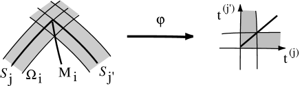
Figure 35. The eikonal flows from the hypersurfaces meeting at a corner and the resulting mapping $\varphi$ giving an edge-corner normal form.

By the above remarks, we can find for each $0<j\leq k$, an $\varepsilon_{j}>0$ so the eikonal flow $\psi_{j}|(S_{j}\times[-\varepsilon_{j},\varepsilon_{j}])$ is a diffeomorphism onto a neighborhood of $x$. We let $\varepsilon=\min\{\varepsilon_{j}\}$. We also let $W=\cap\,\psi_{j}(S_{j}\times(-\varepsilon,\varepsilon))$, which is an open neighborhood of $x$. Then, for each $j=1,\dots,k$ we can define on $W$ a smooth vector field $\zeta_{j}$ by extending $\mathbf{n}_{j}$ along the lines of the eikonal flow in $W$.

By possibly shrinking $W$ the vector fields $\{\zeta_{j}\}$ are linearly independent on $W$. We know that since $\zeta_{j}(x)=\mathbf{n}_{j}$, $\{\zeta_{1}(x^{(1)}),\dots,\zeta_{k}(x^{(k)})\}$ are linearly independent when $x^{(1)}=\dots=x^{(k)}=x$, hence by continuity of the $k$-tuple $(\zeta_{1},\dots,\zeta_{k})$ on the $k$-fold product $W^{k}=W\times\cdots\times W$, there is a neighborhood of $(x,x,\dots,x)$ in $W^{k}$ on which they are linearly independent. This neighborhood contains $W^{\prime\,k}$ for a neighborhood $W^{\prime}$ of $x$. Then, the $\{\zeta_{j}\}$ are the normal vectors to the level hypersurfaces $S_{j\,t}$ in $W$ and hence on $W^{\prime}$. Thus, for any $x^{\prime}\in W^{\prime}$ with $x^{\prime}\in S_{j\,t^{(j)}}$, for each $j$, we conclude they are in general position at $x^{\prime}$. We let $W^{\prime}$ be our desired neighborhood $W$. ∎

Proof of Theorem 4.5.

We first apply Lemma 15.1, where we may furthermore choose compact neighborhoods $x\in W^{\prime\prime}\subset W^{\prime}\subset W$ such that $W^{\prime\prime}$ has diameter $<a=\frac{1}{2}dist(W^{\prime},\,\Omega\backslash W)$, which is positive as $W^{\prime}$ is compact.

Then, we consider $x^{\prime}\in W^{\prime\prime}$. Then, $dist(x^{\prime},S_{j})\leq\varepsilon\leq a$, while $dist(x^{\prime},\mathcal{B}\backslash W)\geq 2a$. Thus, a point $x^{\prime}\in W^{\prime\prime}$ of the Blum medial axis of type $A_{1}^{\ell}$ must have radial distance $\leq\varepsilon$ and has the $A_{1}$ points in $\mathcal{B}\cap W^{\prime\prime}$ which are points in $S_{j}$ which map to $x^{\prime}$ under the eikonal flows $\psi_{j}$.

Thus, the Blum medial axis in $W^{\prime\prime}$ is formed from the transverse intersections of the eikonal flows. The inverse of the $j$-th eikonal flow on $W^{\prime\prime}$ is smooth and given by the mapping $x^{\prime}(=\psi_{j}(x^{(j)},t^{(j)}))\mapsto(x^{(j)},t^{(j)})$. Thus, $t^{(j)}$, $j=1,\dots,k$ are smooth functions on $W^{\prime\prime}$. These define a smooth mapping $\mu:W^{\prime\prime}\to{\mathbb{R}}^{k}$ by $\mu(x^{\prime})=(t^{(1)},\dots,t^{(k)})$. Then, for each subset $J=\{j_{1}<j_{2}\dots<j_{\ell}\}$ with $j_{\ell}\leq k$, we let

$$R^{\ell}_{J}\,=\,\{(t_{1},\dots,t_{k})\in{\mathbb{R}}^{k}:t_{j_{r}}=\min_{j}\{t_{j}\},r=1,\dots,\ell\}.$$

By the general position of the $S_{j\,t}$ and $(1)$ of Lemma 14.1, $\mu$ is transverse to all of the $R^{\ell}_{J}$. Then, the Blum medial axis in $W^{\prime\prime}$ consisting of points of type $A_{1}^{\ell}$ is the disjoint union of the $\mu^{-1}(R^{\ell}_{J})$ for subsets with $card(J)=\ell$.

Furthermore, $Z_{0}=\cap_{j=1}^{k}S_{j}$ is a submanifold of dimension $n+1-k$, and $T_{x}Z_{0}=\cap_{j=1}^{k}T_{x}S_{j}$. This is the subspace orthogonal to the $\mathbf{n}_{j}$. We let $\pi:{\mathbb{R}}^{n+1}\to T_{x}Z_{0}$ denote orthogonal projection. Then, $\pi$ projects $Z_{0}$ submersively onto $T_{x}Z_{0}$ in a neighborhood of $x$, which by shrinking we may assume is $W^{\prime\prime}$. Thus, as $T_{x}Z_{0}=\ker(d\mu(x))$, we conclude that the smooth map $\tilde{\mu}=(\mu,\pi):W^{\prime\prime}\to T_{x}Z_{0}\times{\mathbb{R}}^{k}\simeq{\mathbb{R}}^{n+1}$ is a local diffeomorphism in a neighborhood of $x$. It sends $W^{\prime\prime}\cap\,\Omega$ to a neighborhood of $0$ in $T_{x}Z_{0}\times{\mathbb{R}}_{+}^{k}\simeq{\mathbb{R}}^{n+1-k}\times{\mathbb{R}}_{+}^{k}$, which is the model for a corner $C_{k}$. Hence, $\tilde{\mu}^{-1}$ provides the local $k$–corner model as in Definition 4.4 with $E_{k}$ mapping to the Blum medial axis in a neighborhood of $x$. ∎

Proof of Theorem 4.18 for a Residual Set of Embeddings

We can now complete the proof of Theorem 4.18 for a residual set of embeddings. In the previous section, we have already established the properties i), ii) ,iv) and vi) for a residual set of embeddings $\Phi\in\mathcal{P}$. We have just completed the proof of Theorem 4.5, which establishes the edge-corner normal form for the Blum medial axis at corner points, yielding property iii). Moreover, Theorem 4.5 also shows that there is no linking occurring at corner points, yielding the remainder of condition v). Thus, Theorem 4.18 follows for a residual set of embeddings.

It remains to establish for both Theorem 4.17 and Theorem 4.18 the openness of genericity.

Openness of the Genericity Conditions

We first prove the openness of the genericity conditions for the case of a multi-region configuration $\boldsymbol{\Omega}$ consisting of disjoint compact regions $\Omega_{i}$ with smooth boundaries and without $\tilde{E}_{7}$ points on the medial axes (e.g. there will generically be no $\tilde{E}_{7}$ points for $n+1\leq 6$). This configuration is modeled by $\Phi:\boldsymbol{\Delta}\to{\mathbb{R}}^{n+1}$ and contained in ${\rm int}\,(\tilde{\Omega})$ for a compact region $\tilde{\Omega}$. As earlier $\Omega_{i}=\Phi(\Delta_{i})$, $\mathcal{B}_{i}=\Phi(X_{i})$. We let $\Omega=\coprod_{i}\Omega_{i}$, $X=\coprod_{i}X_{i}$, and $\mathcal{B}=\coprod_{i}\mathcal{B}_{i}$. We suppose it satisfies the genericity conditions with Blum medial axes $M_{i}$ for $\Omega_{i}$ and $M_{0}$ for $\Omega_{0}\cap\tilde{\Omega}$. As $\mathcal{B}$ is a compact (but not connected) smooth hypersurface, we let $\mathbf{n}$ denote the inward pointing unit normal vector field on $\mathcal{B}$. Then, there is an $\varepsilon>0$ such that the eikonal flow $x\mapsto\Phi(x)+t\mathbf{n}(x)$ defines a diffeomorphism $\Psi:X\times[-\varepsilon,\varepsilon]\to{\mathbb{R}}^{n+1}$ onto a tubular neighborhood $T_{\varepsilon}$ of $\mathcal{B}$. For $0<s<\varepsilon$ we denote the image $T_{s}=\Psi(X\times[-s,s])$. We may choose $\varepsilon$ sufficiently small so that $T_{\varepsilon}\subset V\subset{\rm int}\,(\tilde{\Omega})$, for an open subset $V$ containing $\Omega$.

We will use the following Lemma.

Lemma 15.2.

In the above situation, there is an $\varepsilon^{\prime}$ with $0<2\varepsilon^{\prime}<\varepsilon$ and an open neighborhood $\mathcal{U}$ of $\Phi$ in ${\rm Emb}\,(\boldsymbol{\Delta},{\mathbb{R}}^{n+1})$ such that if $\Phi^{\prime}\in\mathcal{U}$, then:

1. $\mathcal{B}^{\prime}=\Phi^{\prime}(X)\subset{\rm int}\,(T_{\varepsilon^{\prime}})$;

2. the eikonal flow for $\mathcal{B}^{\prime}$, $\Psi^{\prime}:X\times[-\varepsilon,\varepsilon]\to{\mathbb{R}}^{n+1}$ is a diffeomorphism onto its image, which is contained in $V\subset{\rm int}\,(\tilde{\Omega})$; and

3. $T_{2\varepsilon^{\prime}}\subset\Psi^{\prime}(X\times[-\varepsilon,\varepsilon])$.

We illustrate the Lemma in Figure 36.

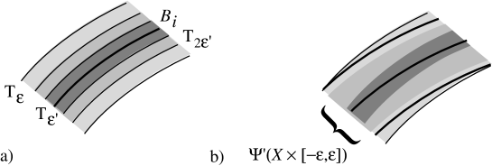
Figure 36. The relation between the tubular neighborhoods of $\mathcal{B}_{i}$ in a) and their images under the perturbation $\Psi$ in b).

After proving Lemma 15.2, we will deduce the consequences for the openness of the genericity conditions for the case of a multi-region configuration consisting of disjoint regions with smooth boundaries.

Proof of Lemma 15.2.

There is a continuous map ${\rm Emb}\,(X,{\mathbb{R}}^{n+1})\to C^{\infty}(X,S^{n})$ sending $\Phi$ to its Gauss map $\mathbf{n}_{\Phi}$, which is given by the inward pointing unit normal vector field. We may combine the two mappings to define a mapping $\Psi^{\prime}(x)=\Phi^{\prime}(x)+t\mathbf{n}_{\Phi^{\prime}}$ on $X\times[-\varepsilon,\varepsilon]\to{\mathbb{R}}^{n+1}$. This defines a continuous mapping in the Whitney topology

$$\tilde{G}:{\rm Emb}\,(\Delta,{\mathbb{R}}^{n+1})\, \rightarrow\,C^{\infty}(X\times[-\varepsilon,\varepsilon],{\mathbb{R}}^{n+1})$$

$$\Phi^{\prime}\, \mapsto\,\Psi^{\prime}.$$

First, as ${\rm int}\,(T_{\varepsilon^{\prime}})$ is an open subset of ${\mathbb{R}}^{n+1}$, the set of smooth mappings with images in ${\rm int}\,(T_{\varepsilon^{\prime}})$ form an open subset $\mathcal{U}_{1}$ of $C^{\infty}(X,{\mathbb{R}}^{n+1})$. Since the restriction map ${\rm Emb}\,(\boldsymbol{\Delta},{\mathbb{R}}^{n+1})\to C^{\infty}(X,{\mathbb{R}}^{n+1})$ is continuous, $\mathcal{U}_{1}$ is pulled back to an open subset $\mathcal{U}_{1}^{\prime}\subset{\rm Emb}\,(\boldsymbol{\Delta},{\mathbb{R}}^{n+1})$. The configuration embeddings in $\mathcal{U}_{1}^{\prime}$ then satisfy condition (1).

Next, for smooth manifolds $N$ and $P$ with $N$ compact, the set of $C^{\infty}$ $1-1$ immersions forms an open subset of $C^{\infty}(N,P)$, see e.g. [GG, Prop. 5.8]. Thus, there is an open subset $\mathcal{U}$ of $C^{\infty}$ $1-1$ immersions in $C^{\infty}(X\times[-\varepsilon,\varepsilon],{\mathbb{R}}^{n+1})$. As $X\times[-\varepsilon,\varepsilon]$ is compact, such an immersion is a diffeomorphism onto its image. Hence, property (2) holds for $\Phi$ in the inverse image of this open set under $\tilde{G}$.

Third, there is an open subset of $C^{\infty}(X\times[-\varepsilon,\varepsilon],{\mathbb{R}}^{n+1})$ containing $\Psi$ which will map $X\times[-\varepsilon,\varepsilon]$ into $V$ and each component of $X\times\{-\varepsilon,\varepsilon\}$ into $(\Omega\backslash{\rm int}\,(T_{2\varepsilon^{\prime}}))\cap{\rm int}\,(\tilde{\Omega})$. For a diffeomorphism $\Psi^{\prime}$ contained in a sufficiently small open set $\mathcal{U}^{\prime\prime}$ containing $\Psi$, it maps each $X_{i}\times\{\pm\varepsilon\}$ to the same complementary components as does $\Psi$. Thus, by a degree argument the image of $\Psi^{\prime}$ must contain $T_{2\varepsilon^{\prime}}$ giving (3). ∎

We now apply Lemma 15.2 to prove openness. We note that openness cannot be deduced from multi-transversality conditions on all of $\mathcal{B}^{(\ell)}$ (by Theorem 13.2 we only obtain openness on a compact subset of $\mathcal{B}^{(\ell)}$). Instead we show that we can pass to the infinitesimal stability of smooth maps associated to the multi-distance and height-distance functions, and apply Mather’s Theorem “Infinitesimal Stability Implies Stability”.

Relation with Infinitesimally Stable Mappings

We first choose the $\varepsilon^{\prime}$ satisfying the Lemma and yielding an open subset $\mathcal{U}\subset{\rm Emb}\,(\boldsymbol{\Delta},{\mathbb{R}}^{n+1})$. Then, for $i>0$ we let $C_{i}^{\prime}=\Omega_{i}\backslash{\rm int}\,(T_{2\varepsilon^{\prime}})$ and $C_{i}=\Omega_{i}\backslash{\rm int}\,(T_{\frac{3}{2}\varepsilon^{\prime}})$. Next, given $\tilde{\Omega}$ we choose compact submanifolds $\tilde{\Omega}_{1}$ and $\tilde{\Omega}^{\prime}$ satisfying

$$\tilde{\Omega}\subset{\rm int}\,(\tilde{\Omega}_{1})\subset\tilde{\Omega}_{1}\subset\tilde{\rm int}\,(\tilde{\Omega}^{\prime})\subset\tilde{\Omega}^{\prime}\,.$$

Then, we replace $\Omega_{0}$ by ${\rm int}\,(\tilde{\Omega}^{\prime})\cap\Omega_{0}$ and still denote it by $\Omega_{0}$. Next, we let $C_{0}^{\prime}=\tilde{\Omega}\backslash{\rm int}\,(T_{2\varepsilon^{\prime}}))$ and $C_{0}=\tilde{\Omega}_{1}\backslash{\rm int}\,(T_{\frac{3}{2}\varepsilon^{\prime}}))$. Third, for $i>0$ we let $U_{i}=\Omega_{i}\backslash(T_{\varepsilon^{\prime}})$ and $U_{0}={\rm int}\,(\tilde{\Omega}^{\prime})$. By Lemma 15.2, for $\Phi^{\prime}\in\mathcal{U}$, the corresponding Blum medial axes satisfy $M_{i}^{\prime}\subset C_{i}$ for $i>0$ and $M_{0}^{\prime}\cap\tilde{\Omega}\subset C_{0}$.

We then have for all $i\geq 0$,

$$C_{i}^{\prime}\,\,\subset\,\,{\rm int}\,(C_{i})\,\,\subset\,\,C_{i}\,\,\subset\,\,U_{i}\,\,\subset\,\,{\rm int}\,(\Omega_{i})$$

with $C_{i}$ and $C_{i}^{\prime}$ compact and $U_{i}$ open.

We will consider various functions related to the distance and height functions associated with the embedding $\Phi$. For $i\geq 0$ we begin with

(15.1) $$\bar{\sigma}_{i}:X_{i}\times{\rm int}\,(\Omega_{i}) \to{\mathbb{R}}\times{\rm int}\,(\Omega_{i})$$

$$(x,u^{(i)})\quad \mapsto\quad(\sigma(x,u^{(i)}),u^{(i)})\,,$$

and

(15.2) $$\bar{\nu}_{i}:X_{i}\times S^{n} \to{\mathbb{R}}\times S^{n}$$

$$(x,v)\quad \mapsto\quad(\nu(x,v),v)\,.$$

Then, via the following general lemma, we relate the local $\mathcal{R}^{+}$-versality of $\sigma_{i}$ and the local $\mathcal{A}$-stability of $\bar{\sigma}_{i}$, $i=0,\dots m$; and similarly for $\nu_{i}$ and $\bar{\nu}_{i}$.

Lemma 15.3.

Suppose $\bar{F}(x,u):{\mathbb{R}}^{n+1}\times U,S\times\{u^{(0)}\}\to{\mathbb{R}},0$ is an unfolding of $f(x):{\mathbb{R}}^{n+1},S\to{\mathbb{R}},0$, where each germ of $f$ at each $x^{(i)}\in S$ is weighted homogeneous. Then, $\bar{F}$ is the $\mathcal{R}^{+}$-versal unfolding of $f$ if and only if

$$F(x,u)=(\bar{F}(x;u),u):{\mathbb{R}}^{n+1}\times U,S\times\{u^{(0)}\}\to{\mathbb{R}}\times U,(0,u^{(0)})$$

is infinitesimally $\mathcal{A}$-stable.

Proof of Lemma 15.3.

In either direction it is sufficient to consider a finite set $S\subset{\mathbb{R}}^{n+1}$ with $u^{(0)}\in U$. We let $S=\{x^{(1)},\dots,x^{(r)}\}$, and choose local coordinates $x^{(j)}_{i}$ about each $x^{(j)}$. We note that points $x^{(j)}$ at which the multigerm is nonsingular can be ignored without affecting the conclusion. We also let $u=(u_{1},\dots u_{q})$ denote the local coordinates for $U$ about $u^{(0)}$, and $y$ a coordinate for ${\mathbb{R}}$. For these coordinates, we let $\bar{F}_{j}$ denote the germ of $\bar{F}$ at $x^{(j)}$. Next, we let $\mathcal{C}_{x^{(j)}}$ denote the ring of germs of functions at $x^{(j)}$ with maximal ideal $\text{\it m}_{x^{(j)}}$, and $\mathcal{C}_{x^{(j)},u}$ the ring of germs at $(x^{(j)},u^{(0)})$, with maximal ideal $\text{\it m}_{x^{(j)},u}$, etc. With $\{\varphi_{1},\dots,\varphi_{k}\}$ understood, we abbreviate a module $R\{\varphi_{1},\dots,\varphi_{k}\}$ by $R\{\varphi_{i}\}$.

Then the infinitesimal stability of $F(x,u):{\mathbb{R}}^{n+1}\times U,S\times\{u^{(0)}\}\to{\mathbb{R}}\times U,(0,u^{(0)})$ is equivalent to

(15.3) $$\sum_{j=1}^{r}\mathcal{C}_{x^{(j)},u}\{\dfrac{\partial\bar{F}_{j}}{\partial x^{(j)}_{i}},\dfrac{\partial}{\partial u_{i}}+\dfrac{\partial\bar{F}_{j}}{\partial u_{i}}\}\,+\mathcal{C}_{y,u}\{\dfrac{\partial}{\partial y},\dfrac{\partial}{\partial u_{i}}\}\,\,=\,\,\oplus_{j=1}^{r}\mathcal{C}_{x^{(j)},u}\{\dfrac{\partial}{\partial y},\dfrac{\partial}{\partial u_{i}}\}$$

where $\mathcal{C}_{y,u}\{\dfrac{\partial}{\partial y},\dfrac{\partial}{\partial u_{i}}\}\,\subset\,\oplus_{j=1}^{r}\mathcal{C}_{x^{(j)},u}\{\dfrac{\partial}{\partial y},\dfrac{\partial}{\partial u_{i}}\}$ is included by the diagonal map $F^{*}$ in each summand. Since $\{\dfrac{\partial}{\partial y},\dfrac{\partial}{\partial u_{i}}+\dfrac{\partial\bar{F}_{j}}{\partial u_{i}},i=1,\dots,q\}$ is also a set of free generators for $\mathcal{C}_{x^{(j)},u}\{\dfrac{\partial}{\partial y},\dfrac{\partial}{\partial u_{i}}\}$, we may project along each $\mathcal{C}_{x^{(j)},u}\{\dfrac{\partial}{\partial u_{i}}+\dfrac{\partial\bar{F}_{j}}{\partial u_{i}}\}$ onto $\mathcal{C}_{x^{(j)},u}\{\dfrac{\partial}{\partial y}\}$ and obtain that (15.3) is equivalent to

(15.4) $$\sum_{j=1}^{r}\mathcal{C}_{x^{(j)},u}\{\dfrac{\partial\bar{F}_{j}}{\partial x^{(j)}_{i}}\}\,+\,\mathcal{C}_{y,u}\{\dfrac{\partial}{\partial y},\dfrac{\partial\bar{F}}{\partial u_{1}},\dots,\dfrac{\partial\bar{F}}{\partial u_{q}}\}\,\,=\,\,\oplus_{j=1}^{r}\mathcal{C}_{x^{(j)},u}\{\dfrac{\partial}{\partial y}\}\,.$$

Then, the system of rings and ideals $(\mathcal{C}_{y,u},\text{\it m}_{u}\mathcal{C}_{y,u})\overset{F_{j}^{*}}{\rightarrow}(\mathcal{C}_{x^{(j)},u},\text{\it m}_{u}\mathcal{C}_{x^{(j)},u})$ is an adequate system of differentiable algebras in the sense of [D6, §6], so by an extension of Mather’s algebraic Lemma to the case of modules over adequate systems of algebras [D6, Lemma 7.3], (15.4) is equivalent to

(15.5) $$\sum_{j=1}^{r}\mathcal{C}_{x^{(j)}}\{\dfrac{\partial f_{j}}{\partial x^{(j)}_{i}}\}\,+\,\mathcal{C}_{y}\{\dfrac{\partial}{\partial y},\dfrac{\partial\bar{F}}{\partial u_{1}}_{|u=u^{(0)}},\dots,\dfrac{\partial\bar{F}}{\partial u_{q}}_{|u=u^{(0)}}\}\,\,=\,\,\oplus_{j=1}^{r}\mathcal{C}_{x^{(j)}}\{\dfrac{\partial}{\partial y}\}\,.$$

As each $f_{j}$ is weighted homogeneous, each $f_{j}\in\mathcal{C}_{x^{(j)}}\{\dfrac{\partial f_{j}}{\partial x^{(j)}_{i}}\}$. Hence

$$\text{\it m}_{y}\{\dfrac{\partial}{\partial y},\dfrac{\partial\bar{F}}{\partial u_{1}}_{|u=u^{(0)}},\dots,\dfrac{\partial\bar{F}}{\partial u_{q}}_{|u=u^{(0)}}\}\,\,\subset\,\,\sum_{j=1}^{r}\mathcal{C}_{x^{(j)}}\{\dfrac{\partial f_{j}}{\partial x^{(j)}_{i}}\}\,.$$

Thus, (15.5) is equivalent to

(15.6) $$\sum_{j=1}^{r}\mathcal{C}_{x^{(j)}}\{\dfrac{\partial f_{j}}{\partial x^{(j)}_{i}}\}\,+\,\langle\dfrac{\partial}{\partial y},\dfrac{\partial\bar{F}}{\partial u_{1}}_{|u=u^{(0)}},\dots,\dfrac{\partial\bar{F}}{\partial u_{q}}_{|u=u^{(0)}}\rangle\,\,=\,\,\oplus_{j=1}^{r}\mathcal{C}_{x^{(j)}}\{\dfrac{\partial}{\partial y}\}\,.$$

This is exactly the equation for the $\mathcal{R}^{+}$-infinitesimal versality of the multigerm $\bar{F}(x,u):{\mathbb{R}}^{n+1}\times U,S\times\{u^{(0)}\}\to{\mathbb{R}},0$, which by the versal unfolding theorem [D6, Thm 9.3] is equivalent to its $\mathcal{R}^{+}$-versality.

As each step is an equivalence, we have established the result. ∎

We apply Lemma 15.3 as follows. Let $\Phi\in\mathcal{P}=(\mathcal{P}_{\sigma\,\rho}\cap\mathcal{P}_{\tau})$, the residual set of mappings of the configuration with the generic properties on $\tilde{\Omega}^{\prime}$ from § 14. Then, the associated distance and height functions are $\mathcal{R}^{+}$-versal unfoldings for any finite set $S\subset X_{i}$. By the Lemma and the results of Mather, this implies that the associated mappings $\bar{\sigma}_{i}$ and $\bar{\nu}_{i}$, which are proper, are infinitesimally stable, as global mappings. This is proven, following Mather, by using a partition of unity argument for the local infinitesimal stability. Then, we want to apply Mather’s theorem “infinitesimal stability implies stability” [M5, Thm 3].

Theorem 15.4 (Mather).

Let $f:N\to P$ be a smooth mapping between manifolds without boundaries and let $M\subset N$ be a closed $0$-codimension submanifold which may have boundaries and corners. Then, if $f|M:M\to P$ is proper and infinitesimally stable, then there is a neighborhood $\mathcal{W}$ of $f|M\in C^{\infty}(M,P)$ and continuous mappings $H_{1}:\mathcal{W}\to{\rm Diff}\,(N)$ and $H_{2}:\mathcal{W}\to{\rm Diff}\,(P)$, with both $H_{1}(f|M)=Id_{N}$ and $H_{2}(f|M)=Id_{P}$, such that

$$g\,\,=\,\,H_{2}(g)\circ f\circ H_{1}(g)\qquad\text{ for all }g\in\mathcal{W}\,.$$

For our situation, we suppose that $M$ is compact with a given compact $M^{\prime}$ with $M^{\prime}\subset{\rm int}\,(M)$. Then, we may shrink $\mathcal{W}$ to a smaller neighhborhood $\mathcal{W}^{\prime}$ in the $C^{\infty}$-topology so that in addition $M^{\prime}\subset H_{1}(g)(M)$.

We apply this version of Mather’s Theorem for each of the mappings $\bar{\sigma}_{i}$ and $\bar{\nu}_{i}$ associated to the given $\Phi$. Each of these mappings is a proper infinitesimally stable mapping. Thus, for each mapping there are open neighborhoods: $\mathcal{V}_{1,i}$ of $\bar{\sigma}_{i}|X_{i}\times C_{i}$ in $C^{\infty}(X_{i}\times C_{i},{\mathbb{R}}\times C_{i})$, and $\mathcal{V}_{2,i}$ of $\bar{\nu}_{i}$ in $C^{\infty}(X_{i}\times S^{n},{\mathbb{R}}\times S^{n})$ satisfying the conclusions of Mather’s Theorem and the additional condition that $M^{\prime}\subset H_{1}(g)(M)$ for each case. However by Lemma 15.3, off of the appropriate compact submanifolds $M^{\prime}$ which denote either $X_{i}\times C_{i}^{\prime}$ or resp. $X_{i}\times S^{n}$, the corresponding mappings have at most stable $A_{1}$ singularities. Also, by Mather’s classification theorem for stable multigerms, the $\mathcal{A}$-equivalence type of the stable multigerms, which are formed from the simple $A_{k}$-germs, are determined by the $\mathcal{R}^{+}$-equivalence class $\Sigma^{(\boldsymbol{\alpha})}$. For any of the mappings $\bar{\sigma}_{i}$ or $\bar{\nu}_{i}$, we denote the set of points of singularity type $\mathbf{A}_{\boldsymbol{\alpha}}$ by $\Sigma^{(\boldsymbol{\alpha})}(\bar{\sigma}_{i})$, or $\Sigma^{(\boldsymbol{\alpha})}(\bar{\nu}_{i})$.

The restriction of the distance mapping to $X_{i}\times C_{i}$ defines a continuous mapping in the Whitney topology $\sigma\mapsto\bar{\sigma}_{i}$,

$$C^{\infty}(X_{i}\times{\mathbb{R}}^{n+1},{\mathbb{R}})\longrightarrow C^{\infty}(X_{i}\times C_{i},{\mathbb{R}}\times C_{i})\,.$$

Hence, there is an open set $\mathcal{U}^{\prime}\subset{\rm Emb}\,(\boldsymbol{\Delta},{\mathbb{R}}^{n+1})$ containing $\Phi$ which maps into each $\mathcal{V}_{i,1}$ and $\mathcal{V}_{i,2}$. Thus, by Lemma 15.3, the associated families of distance and height maps $\sigma_{i}^{\prime}$ or $\nu_{i}^{\prime}$ corresponding to $\Phi^{\prime}\in\mathcal{U}^{\prime}$ are $\mathcal{R}^{+}$-versal unfoldings for any finite set $S\subset X_{i}$. Thus, we obtain openness of the genericity properties of individual stratifications $\Sigma^{(\boldsymbol{\beta}_{i})}$, $\Sigma_{\infty}^{(\boldsymbol{\alpha})}$, and $\Sigma^{(\boldsymbol{\alpha})}$ in $X_{i}$.

We next consider the transverse intersection of the strata $\Sigma^{(\boldsymbol{\alpha})}$ for $\Omega_{0}$ and the $\Sigma^{(\boldsymbol{\beta}_{i})}$ for the $\Omega_{i}$. We form the associated mappings

(15.7) $$\hat{\sigma}_{i,0}:X_{i}\times C_{i}\times C_{0} \to{\mathbb{R}}\times C_{i}\times C_{0}$$

$$(x,u^{(i)},u^{(0)}))\quad \mapsto\quad(\sigma_{i}(x,u^{(i)}),u^{(i)},u^{(0)})\,,$$

(15.8) $$\hat{\sigma}_{0,0}:X_{i}\times C_{i}\times C_{0} \to{\mathbb{R}}\times C_{i}\times C_{0}$$

$$(x,u^{(i)},u^{(0)})\quad \mapsto\quad(\sigma_{0}(x,u^{(0)}),u^{(i)},u^{(0)})\,.$$

These are products of $\bar{\sigma}_{i}$ with identity mappings, so $\Sigma^{(\boldsymbol{\beta}_{j_{p}})}(\hat{\sigma}_{i,0})=\Sigma^{(\boldsymbol{\beta}_{j_{p}})}(\bar{\sigma}_{i})\times C_{0}$ for $i>0$ or $\Sigma^{(\boldsymbol{\alpha})}(\hat{\sigma}_{0,0})=\Sigma^{(\boldsymbol{\alpha})}(\bar{\sigma}_{0})\times C_{i}$. These stratifications are the images under projection of the stratifications $Z^{(\boldsymbol{\beta}_{j_{p}})}$, resp. $Z^{(\boldsymbol{\alpha})}$ in Proposition 14.6. As they are transverse and project diffeomorphically to the strata in the compact manifold (with boundaries and corners) $X_{i}\times C_{i}\times C_{0}$, the strata $\Sigma^{(\boldsymbol{\beta}_{j_{p}})}(\hat{\sigma}_{i,0})$ and $\Sigma^{(\boldsymbol{\alpha})}(\hat{\sigma}_{0,0})$ intersect transversely. They form a closed Whitney stratification of $X_{i}\times C_{i}\times C_{0}$.

Thus, for $\Phi^{\prime}\in\mathcal{U}^{\prime}$ with corresponding $\bar{\sigma}_{i}^{\prime}$ and $\bar{\nu}_{i}^{\prime}$, we may apply Mather’s Theorem and obtain for each $i$ the continuous families of diffeomorphisms $H^{(i)}_{j}(\bar{\sigma}_{i}^{\prime})$, $j=1,2$.

By the properties of the $M^{\prime}$ for $i>0$,

$$H^{(i)}_{1}(\bar{\sigma}_{i}^{\prime})(\Sigma^{(\boldsymbol{\beta}_{j_{p}})}(\bar{\sigma}_{i}))\cap(X_{i}\times C_{i}^{\prime})\,\,=\,\,\Sigma^{(\boldsymbol{\beta}_{j_{p}})}(\bar{\sigma}_{i}^{\prime})\cap(X_{i}\times C_{i}^{\prime})\,\,=\,\,\Sigma^{(\boldsymbol{\beta}_{j_{p}})}(\bar{\sigma}_{i}^{\prime})\,,$$

and similarly

$$H^{(0)}_{1}(\bar{\sigma}_{0}^{\prime})(\Sigma^{(\boldsymbol{\alpha})}(\bar{\sigma}_{0}))\cap(X_{i}\times C_{0}^{\prime})\,\,=\,\,\Sigma^{(\boldsymbol{\alpha})}(\bar{\sigma}_{0}^{\prime})\cap(X_{i}\times C_{0}^{\prime})\,\,=\,\,\Sigma^{(\boldsymbol{\alpha})}(\bar{\sigma}_{i}^{\prime})\,.$$

Thus, from the above, $\Sigma^{(\boldsymbol{\beta}_{j_{p}})}(\hat{\sigma}_{i,0}^{\prime})\cap\Sigma^{(\boldsymbol{\alpha})}(\hat{\sigma}_{0,0}^{\prime})$ is the intersection in $X_{i}\times C_{i}\times C_{0}$ of the pull-back of the closed Whitney stratification with strata $(\Sigma^{(\boldsymbol{\alpha})}(\bar{\sigma}_{i})\times C_{0})\times(\Sigma^{(\boldsymbol{\alpha})}(\bar{\sigma}_{0})\times C_{i})$,by the map

(15.9) $$((H^{(i)}_{1}\times Id_{C_{0}})^{-1},(H^{(0)}_{1}\times Id_{C_{i}})^{-1}):X_{i}\times C_{i}\times C_{0}\longrightarrow(X_{i}\times C_{i}\times C_{0})^{2}\,.$$

By the openness of transversality to closed Whitney stratified sets on compact sets, and the continuous dependence of the mapping (15.9) on $(\bar{\sigma}_{i}^{\prime},\bar{\sigma}_{0}^{\prime})$, and hence on $\Phi^{\prime}$, there is a smaller open neighborhood $\mathcal{U}^{\prime\prime}$ of $\Phi$, such that for $\Phi^{\prime}\in\mathcal{U}^{\prime\prime}$, (15.9) is transverse to the product stratification. Hence, $\Sigma^{(\boldsymbol{\beta}_{j_{p}})}(\bar{\sigma}_{i,0}))$ and $\Sigma^{(\boldsymbol{\alpha})}(\bar{\sigma}_{0,0}^{\prime})$ intersect transversely, and so do their projections in $X_{i}$ by Lemma 14.3. This establishes the openness of the condition that the strata $\Sigma^{(\boldsymbol{\alpha})}$ and $\Sigma^{(\boldsymbol{\beta}_{j_{p}})}$ intersect transversely in each $X_{i}$.

Next, we apply an analogous argument, using

(15.10) $$\check{\sigma}_{i}:X_{i}\times C_{i}\times S^{n} \to{\mathbb{R}}\times C_{i}\times S^{n}$$

$$(x,u^{(i)},v))\quad \mapsto\quad(\sigma_{i}(x,u^{(i)}),u^{(i)},v)\,$$

and

(15.11) $$\check{\nu}_{i}:X_{i}\times C_{i}\times S^{n} \to{\mathbb{R}}\times C_{i}\times S^{n}$$

$$(x,u^{(i)},v)\quad \mapsto\quad(\nu(x,v),u^{(i)},v)\,.$$

We then obtain the openness of the genericity condition of transversality of the strata $\Sigma^{(\boldsymbol{\beta}_{j_{p}})}$ and $\Sigma_{\infty}^{(\boldsymbol{\alpha})}$.

Lastly, we apply the argument a third time to the maps

(15.12) $$\hat{\hat{\sigma}}_{i,0}:X_{i}\times\prod_{i=0}^{m}C_{i} \to{\mathbb{R}}\times\prod_{i=0}^{m}C_{i}$$

$$(x,(u^{(0)},\dots,u^{(m)}))\quad \mapsto\quad(\sigma_{i}(x,u^{(i)}),(u^{(0)},\dots,u^{(m)}))\,$$

to obtain the openness of the genericity condition that the images of the interseections of the strata $\Sigma^{(\boldsymbol{\alpha})}$ and $\Sigma^{(\boldsymbol{\beta}_{j_{p}})}$ intersect in general position in $\Sigma_{M_{0}}^{(\boldsymbol{\alpha})}$.

This completes the proof of openness of the genericity conditions.

Openness of Generic Properties for General Configurations

For the general case, the argument is slightly complicated by the edge-corner points on the common boundaries of regions and the presense of $\tilde{E}_{7}$ points when $n+1=7$. We first allow common boundaries but still exclude $\tilde{E}_{7}$ points. The total space of $\boldsymbol{\Delta}$ is a manifold with boundaries and corners, although the corners are concave rather than convex. We begin with an extension lemma based on an extension result of Bierstone [Bi] .

Lemma 15.5.

If $\tilde{\boldsymbol{\Delta}}$ is an open neighborhood of $\boldsymbol{\Delta}$ in ${\mathbb{R}}^{n+1}$, then there is a continuous extension in the Whitney topology

(15.13) $$\eta:{\rm Emb}\,(\boldsymbol{\Delta},{\mathbb{R}}^{n+1})\longrightarrow C^{\infty}(\tilde{\boldsymbol{\Delta}},{\mathbb{R}}^{n+1})\,.$$

Proof.

In the case of convex corners, Mather proved an extension result giving a continuous extension of smooth functions on an $n$-manifold $M\subset{\mathbb{R}}^{n}$ with boundaries and corners to an open neighborhood $U$ of $M$ in ${\mathbb{R}}^{n}$ (see [M4] and the proposition in [M5, §5]). This method uses continuous local extensions for all $C^{\infty}$ functions in neighborhoods of the corner points, based on the extension method of Seeley [Se], together with a partition of unity. This method also works in our case provided we have a continuous local extension on a neighborhood for the concave corner points. In this case, whether of type $P_{k}$ or $Q_{k}$ the complement in the edge-corner model is the interior of an edge-corner point. The region itself is locally a closed semi-analytic set which is the closure of its interior. This is exactly the situation where the extension result of Bierstone [Bi] applies to give a continuous extension from $C^{\infty}$ functions on the region in a neighborhood of the edge-corner point to an open neighborhood of the point in ${\mathbb{R}}^{n+1}$. With this local extension, we can apply the same argument used by Mather to give the continuous extension (15.13), where $\tilde{\boldsymbol{\Delta}}$ denotes an open neighborhood of $\boldsymbol{\Delta}$. ∎

Then, in $\tilde{\boldsymbol{\Delta}}$ we can extend each nonempty $Cl(X_{i\,j})$ to an open hypersurface $\tilde{X}_{i\,j}$ and then construct a compact submanifold with boundaries and corners $S_{i\,j}$ so that $Cl(X_{i\,j})\subset{\rm int}\,(S_{i\,j})\subset\tilde{X}_{i\,j}$, where ${\rm int}\,(\cdot)$ is taken in the manifold $\tilde{X}_{i\,j}$.

We generally denote $\eta(\Phi)$ by $\tilde{\Phi}$. We choose $\tilde{\boldsymbol{\Delta}}$ small enough so that $\tilde{\Phi}$ is still an embedding. Then, we first restrict to the open subset $\mathcal{U}^{\prime}$ which is the pull-back of the open subset of $C^{\infty}(\tilde{\boldsymbol{\Delta}},{\mathbb{R}}^{n+1})$ consisting of those $\tilde{\Phi}^{\prime}$ which restricted to each $S_{i\,j}$ are embeddings.

We furthermore let $S_{i}=\coprod_{j}S_{i\,j}$ and $S=\coprod_{i}S_{i}$, which is a disjoint union of manifolds with boundaries and corners. Then, $\tilde{\Phi}$ still defines a smooth map denoted $\tilde{\Phi}:S\to{\mathbb{R}}^{n+1}$, which is an embedding. Then, we can proceed as earlier to define the eikonal flow using the inward pointing unit normal vector fields $\mathbf{n}_{i}$ for each $\Omega_{i}$. Again by compactness of each $S_{i\,j}$, there is an $\varepsilon>0$ so that each $\psi_{i\,j}:S_{i\,j}\times[-\varepsilon,\varepsilon]\to{\mathbb{R}}^{n+1}$ is a diffeomorphism onto its image $T_{i\,j,\varepsilon}$ for all $i,j$. Because the singular strata of the boundaries $X_{i}$ form compact sets, we can use the argument in the proof of Theorem 4.5 to find a smaller $\varepsilon>0$ so that in the union $\cup_{i,j}T_{i\,j,\varepsilon}$, the Blum medial axis consists of the edge-corner normal forms for the singular points of $X$.

Then, we replace the tubular neighborhoods $T_{s}$ by the unions $\tilde{T}_{i,s}=\cup_{j}T_{i\,j,s}$ and obtain the analogue of Lemma 15.2.

Lemma 15.6.

In the above situation, there is an $\varepsilon^{\prime}$ with $0<2\varepsilon^{\prime}<\varepsilon$ and an open neighborhood $\mathcal{U}$ of $\Phi$ in ${\rm Emb}\,(\boldsymbol{\Delta},{\mathbb{R}}^{n+1})$ such that if $\Phi^{\prime}\in\mathcal{U}$, then:

1. $\mathcal{B}_{i}^{\prime}=\Phi^{\prime}(X)\subset{\rm int}\,(\tilde{T}_{i,\varepsilon^{\prime}})$;

2. each eikonal flow for $\mathcal{B}_{i}^{\prime}$, $\Psi_{i\,j}^{\prime}:S_{i\,j}\times[-\varepsilon,\varepsilon]\to{\mathbb{R}}^{n+1}$ is a diffeomorphism onto its image; and

3. $\tilde{T}_{i,2\varepsilon^{\prime}}\cap\Omega_{i}\subset\Psi_{i}^{\prime}(S_{i}\times[-\varepsilon,\varepsilon]).$

We again enlarge $\tilde{\Omega}$ via $\tilde{\Omega}_{1}$ to $\tilde{\Omega}^{\prime}$ as earlier and replace $\Omega_{0}$ by $\tilde{\Omega}^{\prime}\cap\Omega_{0}$. With the $\varepsilon^{\prime}$ from Lemma 15.6, we now let $C_{i}^{\prime}=\Omega_{i}\backslash{\rm int}\,(T_{i,2\varepsilon^{\prime}})$ and $C_{0}^{\prime}=\tilde{\Omega}_{1}\cap(\Omega_{0}\backslash{\rm int}\,(T_{0,2\varepsilon^{\prime}}))$. Analogously, we let $C_{i}=\Omega_{i}\backslash{\rm int}\,(T_{i,\frac{3}{2}\varepsilon^{\prime}})$ and $C_{0}=\tilde{\Omega}^{\prime}\cap(\Omega_{0}\backslash{\rm int}\,(T_{0,\frac{3}{2}\varepsilon^{\prime}}))$. Third, we let $U_{i}$ denote ${\rm int}\,(\Omega_{i})\backslash T_{i,\varepsilon}$.

Then, we proceed as earlier. We have the analogous collection of mappings (15.1) - (15.2), (15.7) - (15.8), (15.10) - (15.11), and (15.12), for the corresponding families of distance and height based mappings, where we replace each $X_{i}$ by $X_{\mathcal{J}_{i}}$. First, using Lemma 15.6, we deduce that the stratifications are contained in the model $M^{\prime}$ for each case. Then, we apply Lemma 15.3 to conclude that these mappings are infinitesimally stable. We then apply the same adapted version of Mather’s Theorem for the corresponding mappings to obtain an open neighborhood of $\Phi^{\prime}\in\mathcal{U}^{\prime}$, to which we can repeat the arguments to conclude that the stratifications are closed Whitney stratifications which intersect transversely where appropriate. As earlier, we may conclude that they map diffeomorphically onto the boundary and intersect transversely. This completes the proof of openness of the genericity conditions for the general multi-configuration in the absence of $\tilde{E}_{7}$ points.

Openness of Generic Properties Allowing $\tilde{E}_{7}$ Points

Lastly, we include the possibility of $\tilde{E}_{7}$ points when $n+1=7$. By transversality to the $\tilde{E}_{7}$-stratum, these points will occur at isolated points. Consider points $x_{0}\in X_{i}$ and $u_{0}\in M_{i}$, such that $\sigma(\cdot,u_{0})$ has a minimum $y_{0}$ at $x_{0}$ of type $\tilde{E}_{7}$. By transversality, we may suppose $j_{1}^{4}\sigma(x,u)$ is transverse at $(x_{0},u_{0})$ to the Whitney stratified set defined by the closure of the $\tilde{E}_{7}$-stratum. Then, there is an open neighborhood $\mathcal{U}^{\prime\prime}$ of embeddings and open neighborhoods $u_{0}\in U$ and $x_{0}\in V$ so that for $\Phi^{\prime}\in\mathcal{U}^{\prime\prime}$, the associated distance function $\sigma^{\prime}$ saisfies: $j_{1}^{4}\sigma^{\prime}(x,u)$ transversely meets $\tilde{E}_{7}$-stratum at a unique point $(x^{\prime},u^{\prime})\in V\times U$ and the associated $\sigma^{\prime}(x,u^{\prime})$ has a minimum at $x^{\prime}$. Furthermore, by a result of Looijenga [L2], the transversality to the $\tilde{E}_{7}$ stratum implies that the resulting unfolding at such a point as in (15.1) given by

$$\bar{\sigma}_{i}:X_{i}\times{\rm int}\,(\Omega_{i})\to{\mathbb{R}}\times{\rm int}\,(\Omega_{i})$$

will define a topologically stable mapping near $(x_{0},u_{0})$. Looijenga [L2] shows that the germ is topologically equivalent to the unfolding which is infinitesimally versal except for the modulus term; and the proof of topological stability is given in [D8, Thm 4]. By this we mean: that there is a neighborhood of embeddings, still denoted by $\mathcal{U}^{\prime\prime}$, compact neighborhoods $u_{0}\in D_{1}\subset{\rm int}\,(D_{2})\subset D_{2}\subset U$, $x_{0}\in V_{1}\subset{\rm int}\,(V_{2})\subset V_{2}\subset V$ and $y_{0}\in W_{1}\subset{\rm int}\,(W_{2})\subset W_{2}\subset{\mathbb{R}}$ such that if $\Phi^{\prime}\in\mathcal{U}^{\prime\prime}$, with associated mapping $\bar{\sigma}_{i}^{\prime}$ then:

• there are homeomorphisms onto their images $\varphi=(\varphi_{1},\varphi_{2}):V_{2}\times D_{2}\to\stackrel{{\scriptstyle\circ}}{{X}}_{i}\times U$, and $\psi:W_{2}\times D_{2}\to{\mathbb{R}}\times U$;

• such that $\bar{\sigma}_{i}^{\prime}=\psi\circ\bar{\sigma}_{i}\circ\varphi^{-1}$ on $\varphi(V_{2}\times D_{2})$;

• $\varphi(D_{2}\times V_{2})\supset D_{1}\times V_{1}$, $\psi(W_{2}\times V_{2})\supset W_{1}\times V_{1}$; and

• $\varphi$ is a smooth diffeomorphism on the complement of $(x_{0},u_{0})$ and $\psi$ is a smooth diffeomorphism on the complement of $(y_{0},u_{0})$.

We can repeat this for each $\tilde{E}_{7}$ point for $\sigma_{i}$, and ensure that the above neighborhoods are distinct. If they are labeled by an index $j$, then we can apply the earlier argument after we remove the ${\rm int}\,(D^{(j)}_{1})$ for all $j$. Then, off the union of the $D^{(j)}_{1}$ the generic properites persist in an open neighborhood of $\Phi$. Also, on each $D^{(j)}_{1}$, the medial axis for $\Phi^{\prime}$ will be the image of that of $\Phi$ via the homeomorphism $\varphi$ and will have generic properties off $\varphi_{2}(x_{0},u_{0})$, which must also be an $\tilde{E}_{7}$ point, and hence equals the unique point $(x^{\prime},u^{\prime})$. Thus, the medial axis has generic properties off the $\tilde{E}_{7}$ points; and at these points its structure is topologically constant. Because the $\tilde{E}_{7}$ points are isolated, the codimension conditions and transversality only allow the linking as earlier described, so in this sense the generic properties for $\tilde{E}_{7}$ points hold for an open set of embeddings.

16. Reductions of the Proofs of the Transversality Theorems

We begin the proofs of Theorems 13.1 and 13.2 by first outlining the three main steps of the proofs:

1. reduce Theorem 13.1 to a relative transversality theorem and Theorem 13.2 to a “hybrid transversality theorem”which combines the relative and absolute transversality theorems in [D5];

2. introduce the families of perturbations needed to prove the transversality for the space of mappings and compute the necessary infinitesimal deformations; and

3. verify the transversality conditions for the families of perturbations.

We explain each of these steps in more detail.

The “hybrid transversality theorem”is an extension of Thom’s transversality theorem which applies to a continuous mapping $\Psi:\mathcal{H}\to C^{\infty}(M,N)$, where $\mathcal{H}$ is a Baire space, and $M$ and $N$ are smooth manifolds (where we allow $M$ to have boundaries and corners). We assume there is given a subbundle $\mathcal{H}^{k}(M,N)$ of the jet space $J^{k}(M,N)$ which consists of $k$-jets $j^{k}(\Psi(h))(x)$ for all $h\in\mathcal{H}$ and all $x\in M$. Then, for any $h\in\mathcal{H}$ the associated jet mapping $j^{k}(\Psi(h))(M)\subset\mathcal{H}^{k}(M,N)$. We consider either closed Whitney stratified sets $W\subset\mathcal{H}^{k}(M,N)$ or submanifolds $W$ whose closures form Whitney stratified sets with $W$ a stratum. We refer to the latter $W$ as being “relatively Whitney stratifiable”. Then, by [D5, Thm 1.3] and [D5, Thm 1.5], provided (in an appropriate sense) $\Psi$ is “transverse to $W$”  relative to $\mathcal{H}^{k}(M,N)$, then on any compact subset $C\subset M$ there is an open dense subset of $h\in\mathcal{H}$ for which $j^{k}(\Psi(h))$ is transverse on $C$ to the closed Whitney stratified set determined by $W$. We may alternatively consider the situation where for a closed Whitney stratified set $Y\subset M\backslash E$, with $E\subset M$ a closed subset, $\mathcal{H}^{k}(M\backslash E,N)$ is the restriction of the bundle to $M\backslash E$. If $\Psi$ is “transverse on $Y$ to $W$”  relative to $\mathcal{H}^{k}(M\backslash E,N)$, then, there is a corresponding transversality result that on any compact subset $C\subset M\backslash E$, there is an open dense subset of $h\in\mathcal{H}$ for which $j^{k}(\Psi(h))$ is transverse on $Y\cap C$ to $W$.

We apply either of these results to the geometric mappings that associate to an embedding $\Phi:\boldsymbol{\Delta}\to{\mathbb{R}}^{n+1}$ either the multi-distance functions $\rho_{i}$ or the height-distance function $\tau$. In each case we must verify that “the mapping $\Psi$ is transverse to the appropriate closed Whitney stratified sets”(we recall the definition below). The transversality conditions in Theorem 13.2 are shown to be equivalent to conditions in the setting of the hybrid transversality theorem for the appropriate Whitney stratified sets.

It then remains to show that the corresponding mappings $\Psi$ satisfy the transversality conditions. For this we consider specific families of perturbations of $\Phi$ within ${\rm Emb}\,(\boldsymbol{\Delta},{\mathbb{R}}^{n+1})$ and verify the appropriate local transversality conditions for the families.

Hybrid Transversality Theorem

We give a modified form of [D5, Thms 1.3 and 1.5] for a continuous mapping $\Psi:\mathcal{H}\to C^{\infty}(M,N)$ which is transverse off a closed subset $E\subset M$ to $W\subset\mathcal{H}^{k}(M,N)$, which is either a closed Whitney stratified set or its closure $Cl(W)$ is a Whitney stratified set with $W$ a stratum. While in [D1] $M$ was a smooth manifold, here we allow $M\subset{\mathbb{R}}^{\ell}$ to be a closed stratified set such that $sing(M)\subset E$, a closed subset of $M$. We also let $Y\subset M\backslash E$ be a closed Whitney stratified set. Then, the smoothness of a function $f:M\backslash E\to N$ is still defined.

Definition 16.1.

The map $\Psi$ is said to be transverse or completely transverse to $W\subset\mathcal{H}^{k}(M,N)$ off $E$ if, given an open subset $\mathcal{U}\subset\mathcal{H}$, $x\in M$ and $y\in N$, there are open sets $x\in U\subset M$, and $y\in V\subset N$ such that for every map $h\in\mathcal{U}$, there exists a finite-dimensional smooth manifold $\mathcal{T}\subset\mathcal{U}$ with $h\in\mathcal{T}$ such that for the family

$$\Gamma:M\times\mathcal{T} \rightarrow N,$$

$$(x,f) \mapsto\Psi(f)(x)$$

the $k$-jet extension

$$j^{k}\Gamma:(U\backslash E)\times\mathcal{T} \rightarrow\mathcal{H}^{k}(U\backslash E,N),$$

$$(x,f) \mapsto j^{k}(\Psi(f))(x)$$

is transverse to $W$, respectively transverse to $Cl(W)$, at all points $\{(x,h)\}$ with $x\in U\cap\Psi(h)^{-1}(V)$.

If instead $j^{k}\Gamma|(Y\times\mathcal{T})$ is transverse (on each stratum $Y_{i}\times\mathcal{T}$) to $W$, respectively transverse to $Cl(W)$, at all points $\{(x,h)\}$ with $x\in Y\cap U\cap\Psi(h)^{-1}(V)$, then we say $\Psi$ restricted to $Y$ is transverse or completely transverse to $W$.

Then, for a continuous $\Psi:\mathcal{H}\to C^{\infty}(M,N)$ such that for each $h\in\mathcal{H}$, $j^{k}(\Psi(h)|M\backslash E)$ maps into the subbundle $\mathcal{H}^{k}(M\backslash E,N)=\mathcal{H}^{k}(M,N)\cap J^{k}(M\backslash E,N)$, the hybrid transversality theorem takes the following form.

Theorem 16.2 (Hybrid Transversality Theorem).

Let $E\subset M$ be closed with $Y\subset M\backslash E$ a closed Whitney stratified set. Suppose $W\subset\mathcal{H}^{k}(M\backslash E,N)$ is a closed Whitney stratified subset. If both $\Psi$ and $\Psi$ restricted to $Y$ are transverse to $W$, then for a subset $X\subset M\backslash E$:

• $$\mathcal{W}\,=\,\{h\in\mathcal{H}:j^{k}\Psi(h)\text{ and }j^{k}\Psi(h)|Y\text{ are transverse on $X$ to }W\text{ in }\mathcal{H}^{k}(M\backslash E,N)\}$$

  is open and dense if $X$ is compact and in general is a residual set in the regular $C^{\infty}$–topology;

• in particular, if $W$ is relatively Whitney stratifiable and $X$ is compact then

  $$\tilde{\mathcal{W}}\, =\,\{h\in\mathcal{H}:j^{k}\Psi(h)\text{ and }j^{k}\Psi(h)|Y\text{ are completely transverse on $X$ to }$$

  $$\hskip 36.135ptW\text{ in }\mathcal{H}^{k}(M\backslash E,N)\}$$

  is open and dense in the regular $C^{\infty}$–topology.

Remark 16.3.

The hybrid transversality theorem combines versions of a “relative transversality theorem”, where $j^{k}\Psi(\mathcal{H})=\mathcal{H}^{k}(M,N)$ but for a Whitney stratified set $X\subset M\backslash E$, which requires transversality of ${{}_{s}}j_{1}^{k}(\Psi(h))|X$ to $W$, and an “absolute transversality theorem”, where $\mathcal{H}^{k}(M,N)=J^{k}(M,N)$, but only requires transversality for ${{}_{s}}j_{1}^{k}(\Psi(h))$, possibly on a compact subset (see [D5]). These are formulated so that $\Psi$ can be an operation involving differential or integral operators (as well as geometrically defined mappings) to obtain genericity results for solutions to PDE’s.

The proof of this version of the transversality theorem follows the proof of the relative transversality theorem [D5, Thm 1.3] modifying it to only require that $\Psi$ be transverse to $W$ off $E$ in $\mathcal{H}^{k}(M\backslash E,N)$ as in the absolute transversality theorem [D5, Thm 1.5]. The failure of $Y$ to be smooth on $M$ does not affect the proof.

If we compose $\Psi$ with the continuous mapping $C^{\infty}(M,N)\to C^{\infty}(M^{s},N^{s})$ defined by $f\mapsto f\times\cdots\times f$ and let $E=\Delta^{(s)}M$ we obtain a multi-transversality version of the theorem (extending Corollaries 1.9 and 1.11 given in [D5]). Here recall from §12 the standard notation that $X^{s}=X\times X\times\cdots\times X$ with $s$ factors while $\Delta^{(s)}X$ denotes the generalized diagonal of $X^{s}$. However, to deduce Theorem 13.2 we need a version valid for families of mappings. We apply Theorem 16.2 to deduce a multijet version of the hybrid transversality theorem for families.

Given a smooth mapping $f\in C^{\infty}(M\times Z,N)$, we let ${{}_{s}}j_{1}^{k}(f)(x_{1},\dots,x_{s},z)={{}_{s}}j^{k}(f(\cdot,z)(x_{1},\dots,x_{s})$, with $f(\cdot,z)$ denoting for the fixed value $z\in Z$ the function on $M$. We consider a continuous mapping $\Psi:\mathcal{H}\to C^{\infty}(M\times Z,N)$, and suppose $j_{1}^{k}(\Psi(h))\in\mathcal{H}^{k}(M,N)$. We may define ${{}_{s}}\mathcal{H}^{k}(M,N)$ as the restriction of $(\mathcal{H}^{k}(M,N))^{s}$ to $M^{(s)}\times N^{s}$, yielding ${{}_{s}}\mathcal{H}^{k}(M,N)\subset{{}_{s}}J^{k}(M,N)$. This implies that for $h\in\mathcal{H}$ the map ${{}_{s}}j_{1}^{k}(\Psi(h)):M^{(s)}\times Z\to{{}_{s}}\mathcal{H}^{k}(M,N)$. We may extend Definition 16.1 to the case of $\Psi:\mathcal{H}\to C^{\infty}(M\times Z,N)$. We let $E\subset M^{(s)}$ be a closed subset such that $M^{(s)}\backslash E$ is smooth, and let $Y\subset M^{(s)}\backslash E$ be a closed Whitney stratified subset.

Definition 16.4.

The map $\Psi:\mathcal{H}\to C^{\infty}(M\times Z,N)$ is said to be transverse or completely transverse to $W\subset{{}_{s}}\mathcal{H}^{k}(M,N)$ off $E$ if, given an open subset $\mathcal{U}\subset\mathcal{H}$, $x\in M^{(s)}\backslash E$, $z\in Z$, and $y\in N$, there are open sets $x\in U\subset M^{(s)}\backslash E$, $z\in U^{\prime}\subset Z$, and $y\in V\subset N$ such that for every map $h\in\mathcal{U}$, there exists a finite-dimensional smooth manifold $\mathcal{T}\subset\mathcal{U}$ with $h\in\mathcal{T}$ such that for the family

$$\Gamma:M\times Z\times\mathcal{T} \rightarrow N,$$

$$(x,z,h) \mapsto\Psi(h)(x,z)$$

the $k$-jet extension

$${{}_{s}}j_{1}^{k}(\Gamma):(U\times U^{\prime})\times\mathcal{T} \rightarrow{{}_{s}}\mathcal{H}^{k}(M,N),$$

$$((x_{1},\dots,x_{s}),z,h) \mapsto{{}_{s}}j_{1}^{k}(\Psi(h))((x_{1},z)\dots,(x_{s},z))$$

is transverse to $W$, respectively transverse to $Cl(W)$, relative to ${{}_{s}}\mathcal{H}^{k}(M\backslash E,N)$, at all points $\{((x_{1},\dots,x_{s}),z,h)\}$ with $((x_{1},\dots,x_{s}),z)\in(U\times U^{\prime})\cap\Psi(h)^{-1}(V)$.

If instead ${{}_{s}}j_{1}^{k}(\Gamma)|(Y\times U^{\prime})\times\mathcal{T}$ is transverse (on each stratum $Y_{i}\times\mathcal{T}$) to $W$, respectively transverse to $Cl(W)$, at all points $\{(x,h)\}$ with $x\in((Y\cap U)\times U^{\prime})\cap\Psi(h)^{-1}(V)$, then we say $\Psi$ restricted to $Y$ is transverse or completely transverse to $W$.

Then there is the following multijet version of the Hybrid Transversality Theorem.

Theorem 16.5 (Hybrid Multi-Transversality Theorem).

Let $W\subset{{}_{s}}\mathcal{H}^{(k)}(M,N)$ and $Y\subset M^{(s)}\backslash E$ be closed Whitney stratified sets and let $X\subset M^{(s)}\backslash E$. Suppose that both $\Psi$ and $\Psi$ restricted to $Y$ are transverse to $W$ off $E$. Then, the set

$$\mathcal{W} =\{h\in\mathcal{H}:{{}_{s}}j_{1}^{k}\Psi(h)\text{ and }{{}_{s}}j_{1}^{k}\Psi(h)|(Y\times Z)\text{ are transverse on $X$ to }$$

$$\hskip 224.03743ptW\text{ in }{{}_{s}}\mathcal{H}^{(k)}(M,N)\}$$

is a residual set, and if $X$ is compact, $\mathcal{W}$ is open and dense in the regular $C^{\infty}$–topology.

If $W$ is relatively Whitney stratifiable and $X$ is compact, then

$$\tilde{\mathcal{W}}\, =\,\{h\in\mathcal{H}:{{}_{s}}j^{k}\Psi(h)\text{ and }{{}_{s}}j_{1}^{k}\Psi(h)|(Y\times Z)\text{ are completely transverse on $X$ to }$$

$$\hskip 252.94499ptW\text{ in }{{}_{s}}\mathcal{H}^{k}(M,N)\}$$

is open and dense in the regular $C^{\infty}$–topology.

The proof follows from Theorem 16.2 by composing $\Psi$ with the continuous mapping $C^{\infty}(M\times Z,N)\to C^{\infty}(M^{s}\times Z,N^{s})$ defined by $f\mapsto\tilde{f}$ where $\tilde{f}(x_{1},\dots,x_{s},z)=(f(x_{1},z),f(x_{2},z),\dots,f(x_{s},z))$ and letting $Y\times Z$ be used for $Y$ and $E\cup(\Delta^{(s)}M\times Z)$ be used for $E$ in Theorem 16.2. This yields Theorem 16.5.

Deducing the Transversality Theorems from the Hybrid Transversality Theorems

We will deduce Theorems 13.1 and 13.2 from the preceding hybrid transversality theorems. To do so we must show that Theorems 13.1 and 13.2 can be placed in the frameworks of these transversality theorems.

We first consider Theorem 13.1 and apply Theorem 16.5. If we decompose $X_{i}^{*}$ into connected components $X_{i\,\ell}^{*}$, where $\ell$ is just an index for the components. Then the closure of each $X_{i\,\ell}^{*}$ is a compact manifold with boundaries and corners. We form the disjoint union $\bar{X}_{i}^{*}=\coprod Cl(X_{i\,j}^{*})$, over the connected components of $X_{i}^{*}$. Then, we let $M=(\bar{X}_{i}^{*})^{(s)}\times{\mathbb{R}}^{n+1}$, $N=({\mathbb{R}})^{s}$, and $Y=\Sigma_{Q}\times{\mathbb{R}}^{n+1}$, and $E=\partial(\bar{X}_{i}^{*})^{(s)}\times{\mathbb{R}}^{n+1}$. Also, we let $\mathcal{H}^{k}(M,N)={{}_{s}}J^{k}(\bar{X}_{i}^{*},{\mathbb{R}})$. We define

$$\Psi_{\sigma_{i}}:{\rm Emb}\,(\boldsymbol{\Delta},{\mathbb{R}}^{n+1})\rightarrow C^{\infty}((\bar{X}_{i}^{*})^{(s)}\times{\mathbb{R}}^{n+1},({\mathbb{R}})^{s})$$

such that $\Psi_{\sigma_{i}}(\Phi)$ is defined by $((x_{1},\dots,x_{s}),u)\mapsto(\sigma_{i}(x_{1},u),\dots\sigma_{i}(x_{s},u))$ with $\sigma_{i}$ the distance function associated to $\Phi$ for $X_{i}$. Then, Theorem 16.5 implies the conclusion of Theorem 13.1, once we have shown that $\Psi_{\sigma_{i}}$ is continuous (see Lemma 16.6) and satisfies the perturbation transversality condition in Definition 16.1. This will be verifed in what follows.

Second, we shall also use Theorem 16.5 to prove Theorem 13.2. To do so we must define the setting which applies to the multi-distance and height-distance functions in each case. Given $m>0$ with an assignment $p\mapsto j_{p}$ and a partition $\mathbf{\ell}=(\ell_{1},\dots,\ell_{m})$, we embed $X_{\mathcal{J}_{i}}^{(\mathbf{\ell})}$ in a closed compact manifold with boundaries and corners. First, for any $j$ we let $\bar{X}_{j}=\coprod_{j^{\prime}\in\mathcal{J}_{j}}Cl(X_{j\,j^{\prime}})$, which is a manifold with boundaries and corners such that $\stackrel{{\scriptstyle\circ}}{{X}}_{j}\subset\bar{X}_{j}$ is the smooth interior submanifold. Then, we let $\bar{X}_{\mathcal{J}_{i}}=\coprod_{j\in\mathcal{J}_{i}}\bar{X}_{j}$. Then $\bar{X}_{\mathcal{J}_{i}}$ is a manifold with boundary and corners with interior $X_{\mathcal{J}_{i}}$.

We next extend $X_{\mathcal{J}_{i}}^{(\mathbf{\ell})}$. For the assignment $p\mapsto j_{p}$, and partition $\mathbf{\ell}$, we define

(16.1) $$\bar{X}_{\mathcal{J}_{i}}^{(\mathbf{\ell})}\,\,=\,\,\{(x^{(j_{1})},\dots,x^{(j_{m})})\in\bar{X}_{j_{1}}^{(\ell_{1})}\times\cdots\times\bar{X}_{j_{m}}^{(\ell_{m})}:x_{1}^{(j_{p})}\in X_{i\,j_{p}}\text{ for all $p$}\}$$

Then, we let $M=\bar{X}_{\mathcal{J}_{i}}^{(\mathbf{\ell})}$, which is a manifold with boundaries and corners which contains as a dense open smooth submanifold $X_{\mathcal{J}_{i}}^{(\mathbf{\ell})}$. We may represent $X_{\mathcal{J}_{i}}^{(\mathbf{\ell})}=\bar{X}_{\mathcal{J}_{i}}^{(\mathbf{\ell})}\backslash E$ where $E=\partial M\cup E^{(\mathbf{\ell})}$ with

(16.2) $$E^{(\mathbf{\ell})}\,\, =\,\,\{(x^{(j_{1})},\dots,x^{(j_{m})})\in\bar{X}_{\mathcal{J}_{i}}^{(\mathbf{\ell})}:\text{ there are }p\neq p^{\prime},q,q^{\prime}\text{ so that}$$

$$\qquad\qquad\qquad j_{p}=j_{p^{\prime}},\text{and }x_{q}^{(j_{p})}=x_{q^{\prime}}^{(j_{p^{\prime}})}\}.$$

Here, $E$ is a closed (stratified) set.

First, for the $i$–th multi-distance function we let $Z=({\mathbb{R}}^{n+1})^{(m+1)}$, $N={\mathbb{R}}^{2}$, and define

$$\Psi_{\rho_{i}}:{\rm Emb}\,(\boldsymbol{\Delta},{\mathbb{R}}^{n+1})\rightarrow C^{\infty}(\bar{X}_{\mathcal{J}_{i}}\times({\mathbb{R}}^{n+1})^{(m+1)},{\mathbb{R}}^{2})$$

such that for $j\in\mathcal{J}_{i}$ $\Psi_{\rho_{i}}(\Phi)|\bar{X}_{j_{p}}\times({\mathbb{R}}^{n+1})^{(m+1)}$ applied to $(x,(u^{(j_{1})},\dots,u^{(j_{m})}),u^{(i)})$ equals $(\sigma(x,u^{(i)}),\sigma(x,u^{(j_{p})}))$. This is the smooth extension of the multi-distance function $\rho_{i}$ associated to $\Phi$.

Likewise for the height-distance function we let $Z=({\mathbb{R}}^{n+1})^{(m)}\times S^{n}$, $N={\mathbb{R}}^{2}$, and define

$$\Psi_{\tau}:{\rm Emb}\,(\boldsymbol{\Delta},{\mathbb{R}}^{n+1})\rightarrow C^{\infty}(\bar{X}_{\mathcal{J}_{0}}\times({\mathbb{R}}^{n+1})^{(m)}\times S^{n},{\mathbb{R}}^{2})$$

such that $\Psi_{\tau}(\Phi)|X_{\mathcal{J}_{0}}\times({\mathbb{R}}^{n+1})^{(m)}\times S^{n})=\tau$ and $\Psi_{\tau}(\Phi)$ smoothly extends $\tau$ to the closure $\bar{X}_{\mathcal{J}_{0}}$.

Lemma 16.6.

All of the $\Psi_{\sigma_{i}}$, $\Psi_{\rho_{i}}$, and $\Psi_{\tau}$ are continuous in the Whitney topology (i.e. regular $C^{\infty}$–topology as source spaces are compact).

Proof of Lemma 16.6.

We give the proof for $\Psi_{\rho_{i}}$ and that for $\Psi_{\sigma_{i}}$ and $\Psi_{\tau}$ is similar.

As each restriction $\Phi\mapsto\Phi|\bar{X}_{j_{p}k}$ defines a continuous map ${\rm Emb}\,(\boldsymbol{\Delta},{\mathbb{R}}^{n+1})\to C^{\infty}(\bar{X}_{j_{p}k},{\mathbb{R}}^{n+1})$, the disjoint union over $k$ of the maps gives a continuous map

(16.3) $${\rm Emb}\,(\boldsymbol{\Delta},{\mathbb{R}}^{n+1})\rightarrow C^{\infty}(\bar{X}_{j_{p}},{\mathbb{R}}^{n+1})\,.$$

Second, we may form the product with the identity map on $({\mathbb{R}}^{n+1})^{(m+1)}$ to yield a continuous map in the Whitney topology

(16.4) $$C^{\infty}(\bar{X}_{j_{p}},{\mathbb{R}}^{n+1})\rightarrow C^{\infty}(\bar{X}_{j_{p}}\times({\mathbb{R}}^{n+1})^{(m+1)},{\mathbb{R}}^{n+1}\times({\mathbb{R}}^{n+1})^{(m+1)}).$$

This follows by an argument similar to that in Proposition 3.10 [GG, Chap. 2]. Third, we may compose maps in $C^{\infty}(\bar{X}_{j_{p}}\times({\mathbb{R}}^{n+1})^{(m+1)},{\mathbb{R}}^{n+1}\times({\mathbb{R}}^{n+1})^{(m+1)})$ with the smooth multi-distance map $\sigma_{j}:{\mathbb{R}}^{n+1}\times({\mathbb{R}}^{n+1})^{(m+1)}\to{\mathbb{R}}^{2}$ given by $\sigma_{j}=(\sigma\circ\pi_{m+1},\sigma\circ\pi_{j})$. Here $\pi_{k}$ denotes projection onto the $k$–th factor of $({\mathbb{R}}^{n+1})^{(m+1)}$. As $\sigma_{j}$ is smooth, the composition with $\sigma_{j}$ defines for $j=j_{p}$ a continuous map

(16.5) $$C^{\infty}(\bar{X}_{j_{p}}\times({\mathbb{R}}^{n+1})^{(m+1)},{\mathbb{R}}^{n+1}\times({\mathbb{R}}^{n+1})^{(m+1)})\rightarrow C^{\infty}(\bar{X}_{j_{p}}\times({\mathbb{R}}^{n+1})^{(m+1)},{\mathbb{R}}^{2})$$

(see e.g. Proposition 3.9 of [GG, Chap. 2]).

Then, the composition of (16.3), (16.4), and (16.5) yields a continuous map

(16.6) $${\rm Emb}\,(\boldsymbol{\Delta},{\mathbb{R}}^{n+1})\rightarrow C^{\infty}(\bar{X}_{j_{p}}\times({\mathbb{R}}^{n+1})^{(m+1)},{\mathbb{R}}^{2}).$$

Taking the disjoint unions of these maps over the disjoint $\bar{X}_{j_{p}}\times({\mathbb{R}}^{n+1})^{(m+1)})$ for $p=1,\dots m$ defines a continuous map

(16.7) $${\rm Emb}\,(\boldsymbol{\Delta},{\mathbb{R}}^{n+1})\rightarrow C^{\infty}(\bar{X}_{\mathcal{J}_{i}}\times({\mathbb{R}}^{n+1})^{(m+1)},{\mathbb{R}}^{2}).$$

This is $\Psi_{\rho_{i}}$.

∎

Then, for $\Phi\in{\rm Emb}\,(\boldsymbol{\Delta},{\mathbb{R}}^{n+1})$, $\Psi_{\rho_{i}}(\Phi)$ extends $\rho_{i}$ associated to $\Phi$ and its multijet restricted to $\bar{X}_{\mathcal{J}_{i}}^{(\mathbf{\ell})}\backslash E=X_{\mathcal{J}_{i}}^{(\mathbf{\ell})}$ is contained in ${{}_{s}}\mathcal{H}^{k}(M\backslash E,N)=\,{{}_{\mathbf{\ell}}}E^{(k)}(X_{\mathcal{J}_{i}},{\mathbb{R}}^{2})$. Then, to apply Theorem 16.5 it remains to verify the local transversality condition in Definition 16.4.

For the height-distance function, the argument will be similar except we let $Z=({\mathbb{R}}^{n+1})^{(m)}\times S_{n}$, and ${{}_{s}}\mathcal{H}^{k}(M\backslash E,N)=\,{{}_{\mathbf{\ell}}}E^{(k)}(X_{\mathcal{J}_{0}},{\mathbb{R}}^{2})$ over $X_{\mathcal{J}_{0}}^{(\mathbf{\ell})}$.

Perturbation Transversality Conditions for the Multi-Distance and Height-Distance Functions

We will first consider the case of the multi-distance functions and indicate the modifications that must be applied for the height-distance function. We consider $m>0$ with assignmment $p\mapsto j_{p}$ and partition $\mathbf{\ell}=(\ell_{1},\dots,\ell_{m})$. Suppose $W\subset\,_{\mathbf{\ell}}E^{(k)}(X_{\mathcal{J}_{i}},{\mathbb{R}}^{2})$ is a distinguished submanifold (which is invariant under the action of ${{}_{\mathbf{\ell}}}\mathcal{R}^{+}$). Let $\Phi\in{\rm Emb}\,(\boldsymbol{\Delta},{\mathbb{R}}^{n+1})$, and let $(x,u)\in X_{\mathcal{J}_{i}}\times({\mathbb{R}}^{n+1})^{(m+1)})$ with $x=(x^{(j_{1})},\dots,x^{(j_{m})})$, $x^{(j_{p})}=(x^{(j_{p})}_{1},\dots,x^{(j_{p})}_{\ell_{j_{p}}})$ and $u=(u^{(j_{1})},\dots,u^{(j_{m})},u^{(i)})$. Suppose that the associated multi-distance map $\rho_{i}$ satisfies $\,{}_{\mathbf{\ell}}j_{1}^{k}(\rho_{i})(x,u)\in W$. In the notation of Definition 16.4, we let $N={\mathbb{R}}^{2}$ and $V={\mathbb{R}}^{2}$. Then, we must give a finite dimensional submanifold $\mathcal{T}\subset{\rm Emb}\,(\boldsymbol{\Delta},{\mathbb{R}}^{n+1})$, with $\Phi\in\mathcal{T}$, yielding the finite-dimensional family

(16.8) $$\Gamma:X_{\mathcal{J}_{i}}\times({\mathbb{R}}^{n+1})^{(m+1)}\times\mathcal{T} \rightarrow{\mathbb{R}}^{2}$$

$$(x,u,\Phi^{\prime}) \mapsto\Psi_{\rho_{i}}(\Phi^{\prime})(x,u)=\rho_{i}^{\prime}(x,u)$$

where $\rho_{i}^{\prime}$ is the multi-distance function associated to $\Phi^{\prime}\in\mathcal{T}$. It will have the property that the corresponding partial multi $k$-jet extension

(16.9) $${{}_{\mathbf{\ell}}}j_{1}^{k}\Gamma:X_{\mathcal{J}_{i}}^{(\mathbf{\ell})}\times({\mathbb{R}}^{n+1})^{(m+1)}\times\mathcal{T} \rightarrow{{}_{s}}J^{k}(X_{\mathcal{J}_{i}},{\mathbb{R}}^{2}),$$

$$\;(x,u,\Phi^{\prime}) \mapsto{{}_{\mathbf{\ell}}}j_{1}^{k}\rho_{i}^{\prime}(x,u)$$

is transverse on $U^{(\mathbf{\ell})}\times({\mathbb{R}}^{n+1})^{(m+1)}\times\mathcal{T}$ to $W$ relative to ${{}_{\mathbf{\ell}}}E^{(k)}(X_{\mathcal{J}_{i}},{\mathbb{R}}^{2})$.

We proceed in an analogous fashion for the height function constructing the submanifold $\mathcal{T}$ and corresponding family

(16.10) $$\Gamma:X_{\mathcal{J}_{0}}\times({\mathbb{R}}^{n+1})^{(m)}\times S^{n}\times\mathcal{T} \rightarrow{\mathbb{R}}^{2}$$

$$(x,u,\Phi^{\prime}) \mapsto\Psi_{\tau}(\Phi^{\prime})(x,u)=\tau^{\prime}(x,u)$$

where $\tau^{\prime}$ is the multi-distance function associated to $\Phi^{\prime}$.

In the next section we will construct the submanifolds $\mathcal{T}$ of ${\rm Emb}\,(\boldsymbol{\Delta},{\mathbb{R}}^{n+1})$ using families of perturbations, and verify the required conditions.

17. Families of Perturbations and their Infinitesimal Properties

We begin by giving a general scheme for constructing the submanifolds $\mathcal{T}$ for families of perturbations, and then specialize to those perturbations arising from polynomial mappings.

Construction of the Families of Perturbations

To find an appropriate finite-dimensional manifold $\Phi\in\mathcal{T}\subset{\rm Emb}\,(\boldsymbol{\Delta},{\mathbb{R}}^{n+1})$ which will define a finite family of perturbations, we modify the method used by Looijenga [L] and Wall [Wa] for constructing a family of perturbations in the case of a single distance function. Then, extra care must now be taken in the multi-function case to verify the transversality conditions which will not result from submersions. We shall carry out the local derivative computations for specific families of perturbations using local Monge patches and the algebraic representation of fibers in jet space.

As $\boldsymbol{\Delta}$ is compact, the composition with a smooth embedding $\Phi:\boldsymbol{\Delta}\to{\mathbb{R}}^{n+1}$ defines a continuous map in the Whitney topology (see e.g. [GG, Prop. 3.9, Chap. 2])

$$\Phi^{*}:C^{\infty}({\mathbb{R}}^{n+1},{\mathbb{R}}^{n+1})\longrightarrow C^{\infty}(\boldsymbol{\Delta},{\mathbb{R}}^{n+1})\,.$$

If $T$ is a finite dimensional vector space of smooth mappings in $C^{\infty}({\mathbb{R}}^{n+1},{\mathbb{R}}^{n+1})$, then $\Phi^{*}$ restricts to give a continuous linear map $\Phi^{*}|T:T\to C^{\infty}(\boldsymbol{\Delta},{\mathbb{R}}^{n+1})$. If $\Phi^{*}|T$ is not injective, we can always restrict to a complement to $\ker(\Phi^{*}|T)$. Hence, we suppose $\Phi^{*}|T$ is injective. For example, as $\Phi(\boldsymbol{\Delta})=\boldsymbol{\Omega}$ has non-empty interior, if $T$ is a vector space of polynomial mappings, then $\Phi^{*}|T$ is injective. This gives a submanifold $T^{\prime}=\Phi^{*}(T)\subset C^{\infty}(\boldsymbol{\Delta},{\mathbb{R}}^{n+1})$, as is the translate $T^{\prime\prime}=\Phi+T^{\prime}$. As $\Phi\in{\rm Emb}\,(\boldsymbol{\Delta},{\mathbb{R}}^{n+1})$, which is open in $C^{\infty}(\boldsymbol{\Delta},{\mathbb{R}}^{n+1})$, there is an open subset $\mathcal{T}\subset T^{\prime\prime}$ containing $\Phi$ and lying in ${\rm Emb}\,(\boldsymbol{\Delta},{\mathbb{R}}^{n+1})$.

We will use this method to construct the submanifolds $\mathcal{T}\subset{\rm Emb}\,(\boldsymbol{\Delta},{\mathbb{R}}^{n+1})$ which will satisfy the transversality condition for $\rho_{i}$ and the distinguished submanifolds $W\subset{{}_{\mathbf{\ell}}}E^{(k)}(X_{\mathcal{J}_{i}},{\mathbb{R}}^{2})$.

Perturbation Family from Polynomial Mappings

We recall that for a point in $X_{\mathcal{J}_{i}}^{\mathbf{\ell}}$ the $x^{(j_{p})}$ for each $p$ satisfy $x^{(j_{p})}_{1}\in X_{i\,j_{p}}$. Then, for each $p=1,\dots,m$, we choose disjoint open neighborhoods $U_{j_{p}}^{(q)}\subset{\mathbb{R}}^{n+1}$ of the $x^{(j_{p})}_{q}$ and let $U_{j_{p}}=\prod_{q=1}^{\ell_{p}}U_{j_{p}}^{(q)}$. Likewise, we choose disjoint open neighborhoods $V_{j_{p}}\subset{\mathbb{R}}^{n+1}$ of $u^{(j_{p})}$ and $V_{i}$ of $u^{(i)}$. We note that if there are $j_{p},j_{p^{\prime}}\in\mathcal{T}_{i}$ such that $X_{j_{p}\,j_{p^{\prime}}}\neq\emptyset$, then it is possible that $x^{(j_{p})}_{q}=x^{(j_{p^{\prime}})}_{q^{\prime}}$ for some $q$ and $q^{\prime}$. In this case we choose the neighborhoods $U_{j_{p}}^{(q)}=U_{j_{p^{\prime}}}^{(q^{\prime})}\subset X_{j_{p}\,j_{p^{\prime}}}$. However, there will be different $u^{(j_{p})}$, $u^{(j_{p^{\prime}})}$ and disjoint neighborhoods $V_{j_{p}}$ and $V_{j_{p^{\prime}}}$.

In each $U_{j_{p}}^{(q)}$ we choose a $C^{\infty}$ bump function $\chi_{j_{p}\,q}$ with support in $U_{j_{p}}^{(q)}$ and $\equiv 1$ in a neighborhood of $x^{(j_{p})}_{q}$. For $k>0$ let $\mathcal{P}^{(k)}({\mathbb{R}}^{n+1})$ denote the vector space of polynomial mappings $g:{\mathbb{R}}^{n+1}\to{\mathbb{R}}^{n+1}$ of degree $\leq k$, of the form $g(y)=(g_{1}(y),\dots,g_{n+1}(y))$ with $y=(y_{1},\dots,y_{n+1})$. Then we define vector spaces

$$T^{(k)}_{j_{p}\,q}\,=\,\{\chi_{j_{p}\,q}\cdot g:g\in\mathcal{P}^{(k)}({\mathbb{R}}^{n+1})\}\quad\text{ and }\quad T\,=\,\times_{x^{(j_{p})}_{q}}T^{(k)}_{j_{p}\,q}\,.$$

where the product for $T$ is over distinct points $x^{(j_{p})}_{q}$. So if $x^{(j_{p})}_{q}=x^{(j_{p^{\prime}})}_{q^{\prime}}$, then there is a single perturbation space $T^{(k)}_{j_{p}\,q}=T^{(k)}_{j_{p^{\prime}}\,q^{\prime}}$ which will provide perturbations for each of them in the single neighborhood $U_{j_{p}}^{(q)}=U_{j_{p^{\prime}}}^{(q^{\prime})}$. We shall see in §18 that nonetheless in this case the appropriate perturbation transversality conditions are still satisfied using the perturbation family we are about to define.

As we have described, $\mathcal{T}$ will be an open subset of $T^{\prime\prime}$ containing $\Phi$, giving the corresponding families (16.8) or (16.10). Our desired $U$ will be obtained by shrinking, if necessary, $U=\prod_{p=1}^{m}U_{j_{p}}$. Hence, to determine the effect of elements of $T$, we observe that elements of $T^{(k)}_{j_{p}\,q}$ only affect the open set $U_{j_{p}}^{(q)}$ containing $x^{(j_{p})}_{q}$. Thus these perturbations act independently and we can consider their effects individually.

For a single $x^{(j_{p})}_{q}$, we simplify notation in the derivative calculations that follow and denote it by $x^{(0)}$ and let $y^{(0)}=\Phi(x^{(0)})\in\mathcal{B}$. We locally represent a neighborhood of $\mathcal{B}$ about $y^{(0)}$ using a Monge patch

(17.1) $$(y_{1},\dots,y_{n+1})\,\,=\,\,(x_{1},\dots,x_{n},f(x_{1},\dots,x_{n}))$$

so that $y=\Phi(x)$ locally is given by (17.1), with $y=(y_{1},\dots,y_{n+1})$ denoting coordinates in ${\mathbb{R}}^{n+1}$ and $x=(x_{1},\dots,x_{n})$ denoting local coordinates for $X$ near $x^{(0)}$. We may also suppose in the case of $x^{(0)}=x^{(j_{p})}_{1}$ that the region $\Omega_{i}$ is below the Monge patch graph and $\Omega_{j_{p}}$ above the graph. We may obtain such a form by an orthogonal transformation and a translation; hence, such transformations still send $\mathcal{P}^{(k)}({\mathbb{R}}^{n+1})$ to itself. We use the following notation to describe the generators for $\mathcal{P}^{(k)}({\mathbb{R}}^{n+1})$. Let $\boldsymbol{\alpha}=(\alpha_{1},\dots,\alpha_{n+1})$ be a multi-index, $y^{\boldsymbol{\alpha}}=y^{\alpha_{1}}\cdots y^{\alpha_{n+1}}$, and use the standard notation $|\boldsymbol{\alpha}|=\sum_{j=1}^{n+1}\alpha_{j}$. For the standard basis $\{e_{i}\}$ for ${\mathbb{R}}^{n+1}$ we let $w_{\boldsymbol{\alpha},\ell}(y)=y^{\boldsymbol{\alpha}}e_{\ell}$ (so the $\ell$-th coordinate is $y^{\boldsymbol{\alpha}}$, and the others are $0$). Then a basis for $\mathcal{P}^{(k)}({\mathbb{R}}^{n+1})$ is given by $\{w_{\boldsymbol{\alpha},\ell}:0\leq|\boldsymbol{\alpha}|\leq k\text{ and }0\leq\ell\leq n+1\}$. Thus, any $g(y)\in\mathcal{P}^{(k)}({\mathbb{R}}^{n+1})$ may be written as $g(y)=\sum_{\ell=1}^{n+1}\sum_{|\boldsymbol{\alpha}|\leq k}\,t_{\boldsymbol{\alpha},\ell}\,w_{\boldsymbol{\alpha},\ell}$. We will use $\mathbf{t}=(t_{{\boldsymbol{\alpha},\ell}})$ as coordinates for $\mathcal{P}^{(k)}({\mathbb{R}}^{n+1})$.

By restricting to a sufficiently small neighborhood of $x^{(0)}$ we may assume $\chi\equiv 1$, so sufficiently near $x^{(0)}$, the elements of $T^{\prime}$ have the form

(17.2) $$\tilde{\Phi}\,\,=\,\,\Phi+\sum_{\ell=1}^{n+1}\sum_{|\boldsymbol{\alpha}|\leq k}t_{\boldsymbol{\alpha},\ell}\,w_{\boldsymbol{\alpha},\ell}\circ\Phi\,.$$

Computation of Derivatives for Families of Perturbations

In this section, we use (17.2) to define the perturbed functions associated to $\tilde{\Phi}$ from the basic distance and height functions $\sigma^{\prime}(y,u)=\|y-u\|^{2}$ and $\nu^{\prime}(y,v)=y\cdot v$ on ${\mathbb{R}}^{n+1}$. The perturbed distance function is defined by $\tilde{\sigma}=\sigma^{\prime}\circ(\tilde{\Phi}\times id)$ so that $\tilde{\sigma}(x,u,\mathbf{t})=\|\tilde{\Phi}(x,\mathbf{t})-u\|^{2}$. For a tuple $(u^{(j_{1})},\dots,u^{(j_{m})},u^{(i)})$, we let $\tilde{\sigma}_{j_{p}}(x,\mathbf{t})=\tilde{\sigma}(x,u^{(j_{p})},\mathbf{t})=\|\tilde{\Phi}(x,\mathbf{t})-u^{(j_{p})}\|^{2}$ for each $p$, and also for $i$ in place of $j_{p}$. Second, the perturbed height function $\tilde{\nu}=\nu^{\prime}\circ(\tilde{\Phi}\times id)$ so $\tilde{\nu}(x,v,\mathbf{t})=\tilde{\Phi}(x,\mathbf{t})\cdot v$. Then, from these we define the perturbed multi-distance function $\tilde{\rho}_{i}$ by replacing in (12.1) $\sigma(x,u^{(j_{p})})$ by $\tilde{\sigma}(x,u^{(j_{p})},\mathbf{t})$ for all $p$, and similarly for $i$ in place of $j_{p}$. Likewise, the perturbed height-distance function $\tilde{\tau}$ is defined from (12.2) by replacing $\nu(x,v)$ by $\tilde{\nu}(x,v,\mathbf{t})$, and $\sigma(x,u^{(j_{p})})$ by $\tilde{\sigma}(x,u^{(j_{p})},\mathbf{t})$ for all $p$.

For these we determine the resulting infinitesimal deformations resulting from the perturbation $\tilde{\Phi}$. We progressively proceed from germs and multigerms of the distance and height functions to the multi-distance and height-distance functions. For the derivatives with respect to $u$ we use orthonormal coordinates $(u_{1},\dots,u_{n+1})$ in a neighborhood of $u^{(0)}$. For $v^{(0)}\in S^{n}$, we choose for a neighborhood of $v^{(0)}$ an orthonormal basis $\{v_{j}\}$ for $T_{v^{(0)}}S^{n}$ (so orthogonal to $v^{(0)}$), with coordinates $\mathbf{s}=(s_{1},\dots,s_{n})$ defined by $(s_{1},\dots,s_{n})\mapsto\sum_{j=1}^{n}s_{i}v_{i}+s_{n+1}v^{(0)}$, where $s_{n+1}=\sqrt{1-\sum_{j=1}^{n}s_{i}^{2}}$.

Then, we compute

$$\dfrac{\partial\sigma^{\prime}}{\partial y_{i}}=2(y-u)\cdot e_{i}\qquad \text{ and }\qquad\dfrac{\partial\nu^{\prime}}{\partial y_{i}}=e_{i}\cdot v^{(0)};$$

(17.3) $$\dfrac{\partial\sigma^{\prime}}{\partial u_{i}}=-2(y-u)\cdot e_{i}\qquad \text{ and }\qquad\dfrac{\partial\nu^{\prime}}{\partial s_{i}}=y\cdot(v_{i}-\frac{s_{i}}{s_{n+1}}v^{(0)})\,,$$

where here and below “$\cdot$”denotes dot product on ${\mathbb{R}}^{n+1}$.

Then, we use (17) and the chain rule to compute the derivatives of the perturbations of the distance function $\tilde{\sigma}(\cdot,u^{(0)})$ at $(x^{(0)},u^{(0)})$ and the height function $\tilde{\nu}(\cdot,v^{(0)})$ at $(x^{(0)},v^{(0)})$. To compute the derivatives at $x=0$, $\mathbf{s}=0$, $\mathbf{t}=0$, and $u=u^{(0)}$, we let $z=(x,\mathbf{t},\mathbf{s},u)$ and $z_{0}=(0,0,0,u_{0})$ and obtain

• derivatives of the perturbed distance function :

  $$\dfrac{\partial\tilde{\sigma}}{\partial x_{i}}_{|z=z_{0}}\,\, =\,\,2(\Phi-u^{(0)})\cdot\dfrac{\partial\Phi}{\partial x_{i}}\,;$$

  $$\dfrac{\partial\tilde{\sigma}}{\partial u_{j}}_{|z=z_{0}}\,\, =\,\,-2(\Phi-u^{(0)})\cdot e_{j}\,;$$

  $$\dfrac{\partial\tilde{\sigma}}{\partial t_{{\boldsymbol{\alpha},\ell}}}_{|z=z_{0}}\,\, =\,\,2(\Phi-u^{(0)})\cdot(y^{\boldsymbol{\alpha}}\circ\Phi)e_{\ell}\,;$$

  (17.4) $$\dfrac{\partial\tilde{\sigma}}{\partial s_{j}}_{|z=z_{0}}\,\, =\,\,0\,;$$

  and

• derivatives of the perturbed height function :

  $$\dfrac{\partial\tilde{\nu}}{\partial x_{i}}_{|z=z_{0}}\,\, =\,\,\dfrac{\partial\Phi}{\partial x_{i}}\cdot v^{(0)}\,;$$

  $$\dfrac{\partial\tilde{\nu}}{\partial u_{i}}_{|z=z_{0}}\,\, =\,\,0\,;$$

  $$\dfrac{\partial\tilde{\nu}}{\partial t_{{\boldsymbol{\alpha},\ell}}}_{|z=z_{0}}\,\, =\,\,(y^{\boldsymbol{\alpha}}\circ\Phi)e_{\ell}\cdot v^{(0)}\,;$$

  (17.5) $$\dfrac{\partial\tilde{\nu}}{\partial s_{j}}_{|z=z_{0}}\,\, =\,\,\Phi\cdot v_{j}\,.$$

To evaluate these derivatives, we distinguish whether or not the distance function $\tilde{\sigma}(\cdot,u^{(0)})$ and the height function $\tilde{\nu}(\cdot,v^{(0)})$ have critical points at $x^{(0)}$. For the distance function, the condition for a critical point is that $u^{(0)}$ is lying in the normal line to the surface, which for the Monge patch is the $y_{n+1}$-axis so $u^{(0)}_{j}=0$ for $j\leq n$. Then, the distance function will be of the form (13.6). Thus, it will be an $A_{1}$ point unless $u^{(0)}_{n+1}=\frac{1}{\kappa_{j}}$ for some $j\leq n$ and then it is an $A_{k}$ point with $k\geq 2$. We use the same notation as in (13.6), so for a local maximum we must have $u^{(0)}_{n+1}=\frac{1}{\kappa_{1}}$.

For the height function, the condition is that $v^{(0)}$ is normal to the surface so that $v^{(0)}_{j}=0$ for $j\leq n$, and moreover that $x^{(0)}$ is a maximum for the height function for $v^{(0)}$ requires that $v^{(0)}$ is in the positive $y_{n+1}$-direction.

Evaluating Derivatives of Jet Extension Mappings

Next, we use (i)) and (ii)) to evaluate the derivatives of the jet mappings ${{}_{s}}j_{1}^{k}(\tilde{\sigma})$ and ${{}_{s}}j_{1}^{k}(\tilde{\nu})$. To do so we use the local representation of the partial multijet spaces as products in (12.4) of Definition 12.4.

(17.6) $${{}_{\mathbf{\ell}}}E^{(k)}(X_{\mathcal{J}_{i}},{\mathbb{R}}^{2})\,\,=\,\,\prod_{p=1}^{m}\,{{}_{\ell_{p}}}J^{k}(\stackrel{{\scriptstyle\circ}}{{X}}_{j_{p}},{\mathbb{R}}^{2})\,|\,(X_{\mathcal{J}_{i}})^{(\mathbf{\ell})}\,.$$

Furthermore, the multijet space ${{}_{\ell_{p}}}J^{k}(\stackrel{{\scriptstyle\circ}}{{X}}_{j_{p}},{\mathbb{R}}^{2})$ is itself locally a product of jet spaces $J^{k}(X_{i\,j_{p}},{\mathbb{R}}^{2})$ and the jet mapping acts as a product when we fix a value in ${\mathbb{R}}^{n+1}_{i}$ or $S^{n}$:

$$j_{1}^{k}(\tilde{\sigma}):U_{j_{p}}^{(q)}\times V_{j_{p}}\times T_{j_{p}}^{(q)} \longrightarrow J^{k}(U_{j_{p}}^{(q)},{\mathbb{R}})\,\,\simeq\,\,U_{j_{p}}^{(q)}\times{\mathbb{R}}\times J^{k}(n,1)\,,$$

(17.7) $$j_{1}^{k}(\tilde{\nu}):U_{j_{p}}^{(q)}\times S^{n}\times T_{j_{p}}^{(q)} \longrightarrow J^{k}(U_{j_{p}}^{(q)},{\mathbb{R}})\,\,\simeq\,\,U_{j_{p}}^{(q)}\times{\mathbb{R}}\times J^{k}(n,1)\,.$$

As usual $J^{k}(n,1)$ denotes the $k$-jets of germs ${\mathbb{R}}^{n},0\to{\mathbb{R}},0$, and $J^{k}(n,1)\times{\mathbb{R}}\simeq\mathcal{C}_{x}\backslash\text{\it m}^{k+1}$, where $\mathcal{C}_{x}$ denotes the ring of germs on $({\mathbb{R}}^{n},0)$ with maximal ideal m. A $\mathcal{R}^{+}$-invariant submanifold $W$ of (multi-)jet space is a bundle over the base with fiber $W_{0}$. For a local representation of the jet bundle as a product, let $\pi_{f}$ denote projection of the jet bundle onto a fiber. Then, transversality of a multijet map ${{}_{s}}j_{1}^{k}(\psi)$ to $W$ is equivalent to transversality of $\pi_{f}\circ{{}_{s}}j_{1}^{k}(\psi)$ to the fiber $W_{0}$. We refer to $\pi_{f}\circ{{}_{s}}j_{1}^{k}(\psi)$ as the fiber jet extension map, which we denote by ${{}_{s}}j_{f}^{k}(\psi)$.

If $w$ denotes any of the local coordinates and $\psi$ denotes either the distance or height function, then as partial derivatives commute, the fiber jet extension maps can be computed by

(17.8) $$dj_{f}^{k}(\psi)_{|z=z_{0}}(\dfrac{\partial}{\partial w})\,\,=\,\,\dfrac{\partial\psi}{\partial w}_{|z=z_{0}}\quad{\rm mod}\;\text{\it m}^{k+1}.$$

This reduces the verification of the transversality conditions to $W$ in Definitions 16.1 and 16.4 to verifying the transversality of the appropriate fiber jet extension map to the fiber $W_{0}$.

We first use (i)) and (ii)) in (17.8) to compute the derivatives for the Monge patch in the case that $\tilde{\sigma}(\cdot,u^{(0)})$ and $\tilde{\nu}(\cdot,v^{(0)})$ have critical points at $0$. As $\Phi$ is of the form (13.5), $\dfrac{\partial\Phi}{\partial x_{i}}=e_{i}+\dfrac{\partial f}{\partial x_{i}}e_{n+1}$. Evaluating (i)) and (ii)), using the conditions on $u^{(0)}$ and $v^{(0)}$ for critical points, we obtain the following:

• derivatives of the distance function at a critical point:

  $$\dfrac{\partial\tilde{\sigma}}{\partial x_{i}}_{|z=z_{0}}\,\, =\,\,2(x_{i}+(f-u^{(0)}_{n+1})\dfrac{\partial f}{\partial x_{i}})\,;$$

  (17.11) $$\dfrac{\partial\tilde{\sigma}}{\partial u_{j}}_{|z=z_{0}}\,\, =\,\,\left\{\begin{array}[]{lr}-2x_{j}&\displaystyle 0\leq j\leq n\\ -2(f-u^{(0)}_{n+1})&\displaystyle j=n+1\end{array}\right.\,;$$

  (17.14) $$\dfrac{\partial\tilde{\sigma}}{\partial t_{{\boldsymbol{\alpha},\ell}}}_{|z=z_{0}}\,\, =\,\,\left\{\begin{array}[]{lr}2x_{j}(y^{\boldsymbol{\alpha}}\circ\Phi)&\displaystyle 0\leq\ell\leq n\\ 2(f-u^{(0)}_{n+1})(y^{\boldsymbol{\alpha}}\circ\Phi)&\displaystyle\ell=n+1\end{array}\right.\,;$$

  (17.15) $$\dfrac{\partial\tilde{\sigma}}{\partial v_{j}}_{|z=z_{0}}\,\, =\,\,0\,;$$

  and

• derivatives of the height function at a critical point:

  $$\dfrac{\partial\tilde{\nu}}{\partial x_{i}}_{|z=z_{0}}\,\, =\,\,\dfrac{\partial f}{\partial x_{i}}\,;$$

  $$\dfrac{\partial\tilde{\nu}}{\partial u_{i}}_{|z=z_{0}}\,\, =\,\,0\,;$$

  (17.18) $$\dfrac{\partial\tilde{\nu}}{\partial t_{{\boldsymbol{\alpha},\ell}}}_{|z=z_{0}}\,\, =\,\,\left\{\begin{array}[]{lr}0&\displaystyle 0\leq\ell\leq n\\ (y^{\boldsymbol{\alpha}}\circ\Phi)&\displaystyle\ell=n+1\end{array}\right.\,;$$

  (17.19) $$\dfrac{\partial\tilde{\nu}}{\partial v_{j}}_{|z=z_{0}}\,\, =\,\,x_{j}\,.$$

Multijet Properties Implying Stratification Properties on the Boundaries

Before completing the proofs of the transversality theorems, we first take a brief detour to use these calculations to give the proofs of several Lemmas referred to in §14. These Lemmas were used there to prove certain stratification properties of the strata in the boundaries of the regions corresponding to the Blum types.

Specifically we consider the infinitesimal deformations of the multigerms of either multi-distance or height-distance functions arising from the variation of either $u$ or $v$ and all but one of the multigerm points on the boundary. In these cases, $\mathbf{t}=0$ so we are considering the derivative calculations as they apply to $\sigma$ and $\nu$.

We then prove that on the inverse images of certain classes of submanifolds $W^{(\boldsymbol{\alpha})}$ under the (multi)jet maps, these functions are not singular.

Lemma 17.1.

Suppose the distance function $\sigma$ defines the $\mathcal{R}^{+}$–versal unfolding at $x=\{x^{(1)},\dots,x^{(s)}\}$ and $u=u^{(0)}$ of the multigerm $g(x)=\sigma(x,u^{(0)})$ of type $A_{\boldsymbol{\alpha}}$. If either $s>1$, or $s=1$ and $\boldsymbol{\alpha}=(k)$ with $k\geq 2$, then

$$d{{}_{s}}j_{1}^{k}(\sigma)(x,u^{(0)})(\oplus_{j=2}^{s}T_{x^{(j)}}X\oplus T_{u^{(0)}}R^{n+1})\,\cap\,T_{{{}_{s}}j_{1}^{k}(g)(x)}W^{(\boldsymbol{\alpha})}\,\,=\,\,0\,.$$

There is an analogous result for the height function.

Lemma 17.2.

Suppose the height function $\nu$ defines the $\mathcal{R}^{+}$–versal unfolding at $x=\{x^{(1)},\dots,x^{(s)}\}$ and $v=v^{(0)}$ of the multigerm $h(x)=\nu(x,v^{(0)})$ of type $A_{\boldsymbol{\alpha}}$. If either $s>1$, or $s=1$ and $\boldsymbol{\alpha}=(k)$ with $k\geq 2$, then

$$d{{}_{s}}j_{1}^{k}(\nu)(x,v^{(0)})(\oplus_{j=2}^{s}T_{x^{(j)}}X\oplus T_{v^{(0)}}S^{n})\,\cap\,T_{{{}_{s}}j_{1}^{k}(h)(x)}W^{(\boldsymbol{\alpha})}\,\,=\,\,0\,.$$

Note that these lemmas are equally valid replacing the first factor by any other.

A third property involves the Thom-Boardman strata.

Lemma 17.3.

Suppose the distance function $\sigma$, resp. the height function $\nu$, defines the $\mathcal{R}^{+}$–versal unfolding at $x=\{x^{(1)},\dots,x^{(s)}\}$ for $u=u^{(0)}$ of the germ $g(x)=\nu(x,u^{(0)})$, resp. for $v=v^{(0)}$ of the germ $h(x)=\nu(x,v^{(0)})$. If these germs are of Thom-Boardman type $\Sigma_{n,1}$ then

$$dj_{1}^{k}(\sigma)(x,u^{(0)})(T_{u^{(0)}}R^{n+1})\,\cap\,T_{j_{1}^{k}(g)(x)}\Sigma_{n,1}\,\, =\,\,0\,,$$

(17.20) $$dj_{1}^{k}(\nu)(x,v^{(0)})(T_{v^{(0)}}S^{n})\,\cap\,T_{j_{1}^{k}(h)(x)}\Sigma_{n,1}\,\, =\,\,0\,.$$

Proof of Lemma 17.1.

We first consider the case when $s=1$ and use the Monge patch given by (17.1). By (i)),

(17.21) $$dj_{1}^{k}(\sigma)(0,u^{(0)})(T_{u^{(0)}}R^{n+1})\,\,=\,\,\langle-2x_{1},\dots-2x_{n},-2(f-u^{(0)}_{n+1})\rangle\,.$$

For this Monge patch, the distance function $g(x)=\sigma(x,u^{(0)})$ has the form (13.6).

(17.22) $$g(x)\,\, =\,\,\sum_{i=1}^{n}(1-u^{(0)}_{n+1}\kappa_{i})x_{i}^{2}-2u_{0,n+1}\sum_{|\boldsymbol{\alpha}|\geq 3}a_{\boldsymbol{\alpha}}x^{\boldsymbol{\alpha}}+(u^{(0)}_{n+1})^{2}$$

$$\qquad\qquad+\,(\sum_{i=1}^{n}\frac{1}{2}\kappa_{i}x_{i}^{2}\,+\,\sum_{|\boldsymbol{\alpha}|\geq 3}a_{\boldsymbol{\alpha}}x^{\boldsymbol{\alpha}})^{2}.$$

Hence, as $g$ is an $A_{k}$ with $k\geq 2$, $u^{(0)}_{n+1}=\frac{1}{\kappa_{i}}$ for some $i$. For simplicity we assume $i=1$; then

(17.23) $$T\mathcal{R}^{+}\cdot g\,\,\subset\,\,\langle 1\rangle\,+\,\text{\it m}_{x}(x_{2},\dots,x_{n})+\text{\it m}_{x}^{3}\,.$$

Then, since $\kappa_{1}\neq 0$, $f$ has a nonzero term $x_{1}^{2}$, and so the RHS of (17.21) is a complement of dimension $n+1$ to the subspace of $\mathcal{C}_{x}$ given by the RHS of (17.23). Hence, its intersection with the subspace $T\mathcal{R}^{+}\cdot g$ is $0$.

Next, suppose that $s>1$. We let $x_{0}=(x^{(1)}_{0},\dots,x^{(s)}_{0})\subset\stackrel{{\scriptstyle\circ}}{{X}}^{(s)}$ and $g(x)=\sigma(x,u^{(0)})$. Let $g_{j}$ denote the germ of $g$ at $x^{(j)}_{0}$ expressed in terms of a local Monge patch in a neighborhood $U_{j}$ about $x^{(j)}_{0}$ with local coordinates $(x^{(j)}_{1},\dots,x^{(j)}_{n})$. We suppose that the multigerm of $g$ at $x_{0}$ is of type $\boldsymbol{\alpha}=(\alpha_{1},\dots\alpha_{s})$. To simplify notation, we let $z_{j}=j^{k}(g_{j})(x^{(j)})$, $z=(z_{1},\dots,z_{s})$, $z^{\prime}=(z_{2},\dots,z_{s})$, $x^{\prime}_{0}=(x^{(2)}_{0},\dots,x^{(s)}_{0})$ and $\boldsymbol{\alpha}^{\prime}=(\alpha_{2},\dots\alpha_{s})$. We note that $z={{}_{s}}j_{1}^{k}(\sigma)(x_{0},u^{(0)})$.

To prove the Lemma in this case it is sufficient to show that for a set of generators $\{w_{i}\}$ of $\oplus_{j=2}^{s}T_{x^{(j)}}X\oplus T_{u^{(0)}}R^{n+1}$, that $\{d{{}_{s}}j_{1}^{k}(\sigma)(x_{0},u^{(0)})(w_{i})\}$ are linearly independent in $T_{z}\,{{}_{s}}J^{k}(\stackrel{{\scriptstyle\circ}}{{X}},{\mathbb{R}})/T_{z}W^{(\boldsymbol{\alpha})}$. We use the set of generators

$$\{\dfrac{\partial}{\partial x^{(j)}_{i}},j=2,\dots,s,i=1,\dots,n;\dfrac{\partial}{\partial u_{i}},i=1,\dots,n+1\}.$$

We first note that for any $g_{j}$ of type $A_{\alpha_{j}}$, that $\{\dfrac{\partial g_{j}}{\partial x^{(j)}_{1}},\dots,\dfrac{\partial g_{j}}{\partial x^{(j)}_{n}}\}$ form a regular sequence in $\mathcal{C}_{x^{(j)}}$; and hence are linearly independent ${\rm mod}\;\text{\it m}_{x^{(j)}}(\dfrac{\partial g_{j}}{\partial x^{(j)}_{1}},\dots,\dfrac{\partial g_{j}}{\partial x^{(j)}_{n}})$. Thus, in $J^{k}(U_{j},{\mathbb{R}})\simeq U_{j}\times{\mathbb{R}}\times(\text{\it m}_{x^{(j)}}/\text{\it m}_{x^{(j)}}^{k+1})$,

$$dj^{k}(g_{j})(T_{x^{(j)}_{0}}X)\quad\text{is spanned by }\{\dfrac{\partial}{\partial x^{(j)}_{i}}+\dfrac{\partial g_{j}}{\partial x^{(j)}_{i}},i=1,\dots,n\},$$

which are linearly independent in $T_{z_{j}}J^{k}(U_{j},{\mathbb{R}})/T_{z_{j}}W^{(\alpha_{j})}$. Thus, $\{\dfrac{\partial g_{j}}{\partial x^{(j)}_{i}},j=2,\dots,s,\,i=1,\dots,n\}$ are linearly independent in $T_{z^{\prime}}\,{{}_{(s-1)}}J^{k}(\stackrel{{\scriptstyle\circ}}{{X}},{\mathbb{R}})/T_{z^{\prime}}W^{(\boldsymbol{\alpha}^{\prime})}$. Hence,

$$\{\dfrac{\partial g_{j}}{\partial x^{(j)}_{i}},j=2,\dots,s,\,i=1,\dots,n;\,\dfrac{\partial(g_{1},\dots,g_{s})}{\partial u_{i}},i=1,\dots,n+1\}$$

are linearly dependent in $T_{z}\,{{}_{s}}J^{k}(\stackrel{{\scriptstyle\circ}}{{X}},{\mathbb{R}})/T_{z}W^{(\boldsymbol{\alpha})}$ if and only if $\{\dfrac{\partial(g_{1},\dots,g_{s})}{\partial u_{i}},i=1,\dots,n+1\}$ together with $(1,\dots,1)$ are linearly dependent in

$$\mathcal{C}_{x^{(1)}}/(T\mathcal{R}^{+}g_{1})\oplus_{j=2}^{s}\mathcal{C}_{x^{(j)}}/(\dfrac{\partial g_{j}}{\partial x^{(j)}_{1}},\dots,\dfrac{\partial g_{j}}{\partial x^{(j)}_{n}})\,.$$

As $(\dfrac{\partial g_{j}}{\partial x^{(j)}_{1}},\dots,\dfrac{\partial g_{j}}{\partial x^{(j)}_{n}})\subset\text{\it m}_{x^{(j)}}$, it is sufficient to show that $\{\dfrac{\partial(g_{1},\dots,g_{s})}{\partial u_{i}},i=1,\dots,n+1\}$ together with $(1,\dots,1)$ are linearly independent in

(17.24) $$L\,\,=\,\,\mathcal{C}_{x^{(1)}}/(T\mathcal{R}^{+}g_{1})\oplus_{j=2}^{s}\mathcal{C}_{x^{(j)}}/\text{\it m}_{x^{(j)}}.$$

Now

$$\dfrac{\partial g_{j}}{\partial u_{i}}\,\,=\,\,\left\{\begin{array}[]{lr}-2x^{(j)}_{i}&\displaystyle i\leq n,\\ -2(g_{j}-u^{(j)}_{0\,n+1})&\displaystyle i=n+1\end{array}\right.$$

where $u^{(j)}_{0}$ is the point $u^{(0)}$ in the coordinates $x^{(j)}$. Then,

$$\dfrac{\partial(g_{1},\dots,g_{s})}{\partial u_{i}}\,\equiv\,(-2x_{i},0,\dots,0)\quad{\rm mod}\;L\qquad\text{ for }i=1,\dots,n$$

and

$$\dfrac{\partial(g_{1},\dots,g_{s})}{\partial u_{n+1}}\,\equiv\,(-2(g_{j}-u^{(0)}_{n+1}),2u^{(2)}_{0\,n+1},\dots,2u^{(s)}_{0\,n+1})\quad{\rm mod}\;L\,.$$

If $\alpha_{1}\geq 2$, then we can apply the same argument for the case $s=1$ to conclude that these together with $(1,\dots,1)$ are linearly independent in $L$.

If instead $\alpha_{1}=1$, we examine the relations for the first two coordinates in $L$. Again there are two cases based on whether $u^{(0)}-x^{(1)}$ and $u^{(0)}-x^{(2)}$ are or are not collinear. First, if $u^{(0)}-x^{(1)}$ and $u^{(0)}-x^{(2)}$ are not collinear, then they span a plane $P$ which intersects each tangent plane in a line. We choose an orthonormal basis $\{e_{i},i=1,\dots,n-1\}$ for the orthogonal complement to the line. For the tangent plane at $x^{(1)}$ we let $e_{n}$ be a unit vector in the line, and $e_{n+1}$ be along $u^{(0)}-x^{(1)}$. For the second tangent plane we let $e_{i}^{\prime}=e_{i},i=1,\dots,n-1$, $e_{n}^{\prime}$ be along the line of intersection of $P$ with the tangent plane and $e_{n+1}^{\prime}$ be along $u^{(0)}-x^{(1)}$ so that $\{e_{n}^{\prime},e_{n+1}^{\prime}\}$ have the same orientation in $P$ as does $\{e_{n},e_{n+1}\}$. Hence, there is a rotation by an angle $\theta$ sending $\{e_{n}^{\prime},e_{n+1}^{\prime}\}$ to $\{e_{n},e_{n+1}\}$. By (17.21) applied to each germ $g_{j}$, and $i=1,\dots,n-1$,

(17.25) $$d{{}_{2}}j_{1}^{k}(\sigma)((x^{(1)},x^{(2)}),u^{(0)})(e_{i})\,\equiv\,\,(-2x^{(1)}_{i},0)\quad{\rm mod}\;\text{\it m}_{x^{(1)}}^{2}\oplus\text{\it m}_{x^{(2)}}\,.$$

It suffices to show that $d{{}_{2}}j_{1}^{k}(\sigma)((x^{(1)},x^{(2)}),u^{(0)})(e_{i})$ for $i=1,\dots,n+1$ and $(1,1)$ are linearly independent in $\mathcal{C}_{x^{(1)}}/\text{\it m}_{x^{(1)}}^{2}\oplus\mathcal{C}_{x^{(2)}}/\text{\it m}_{x^{(2)}}$. Already (17.25) shows this is true for $i<n$. For $\{e_{n},e_{n+1}\}$, we use (17.21) for $g_{0}$, and (17.21), but for $g_{1}$, together with

$$e_{n}\,\, =\,\,\cos(\theta)e_{n}^{\prime}\,+\,\sin(\theta)e_{n+1}^{\prime}\,,$$

(17.26) $$e_{n+1}\,\, =\,\,-\sin(\theta)e_{n}^{\prime}\,+\,\cos(\theta)e_{n+1}^{\prime}\,.$$

We obtain ${\rm mod}\;\text{\it m}_{x^{(1)}}^{2}\oplus\text{\it m}_{x^{(2)}}$

$$d{{}_{2}}j_{1}^{k}(\sigma)((x^{(1)},x^{(2)}),u^{(0)})(e_{n}) \equiv-2(x_{n}^{(1)},-\sin(\theta)u^{(1)}_{n+1}),$$

(17.27) $$d{{}_{2}}j_{1}^{k}(\sigma)((x^{(1)},x^{(2)}),u^{(0)})(e_{n+1}) \equiv-2(-u^{(0)}_{n+1},-\cos(\theta)u^{(1)}_{n+1})\,.$$

In the subspace spanned by $\{(x_{n}^{(1)},0),(1,0),(0,1)\}$, as $\cos(\theta)\neq 1$, the two terms in (17) together with the term $(1,1)$ are checked to be linearly independent. These together with those in (17.25) are linearly independent in $\mathcal{C}_{x^{(1)}}/\text{\it m}_{x^{(1)}}^{2}\oplus\mathcal{C}_{x^{(2)}}/\text{\it m}_{x^{(2)}}$. This gives the result in this case. The case when $u^{(0)}-x^{(1)}$ and $u^{(0)}-x^{(2)}$ are collinear is easier as we may let $e_{n}^{\prime}=e_{n}$ and $e_{n+1}^{\prime}=-e_{n+1}$ so that (17.25) holds for $i\leq n$ and (17) becomes

$$d{{}_{2}}j_{1}^{k}(\sigma)((x^{(1)},x^{(2)}),u^{(0)})(e_{n+1})\equiv-2(-u^{(0)}_{n+1},u^{(1)}_{n+1}).$$

As $u^{(0)}_{n+1}$ and $u^{(1)}_{n+1}$ have the same sign, this term and $(1,1)$ are linearly independent so again the result is true.

∎

Proof of Lemma 17.2.

The proof here is similar but much easier. Again for $s=1$, we use the Monge patch in (17.1) so $v^{(0)}=e_{n+1}$, and $T_{v^{(0)}}S^{n}$ is spanned by the orthonormal basis $\{e_{i},i=1,\dots,n\}$. By (ii)),

$$\dfrac{\partial\nu}{\partial v_{j}}_{|(x,\mathbf{t})=(0,0)}\,\,=\,\,x_{j}\quad\text{ for }j=1,\dots,n\,.$$

Hence, its intersection with the subspace $T\mathcal{R}^{+}\cdot h$ is $0$. If $s>1$, the case $\alpha_{1}\geq 2$ reduces to an argument analogous to the case $s=1$. If $\alpha_{1}=1$ we again consider the first two factors. Now we may use the same orthogonal basis for the multigerm $h$ at $\{x^{(1)},x^{(2)}\}$ (using the same notation and Monge patches as in the preceding proof). We obtain in place of (17.25) for $i=1,\dots n$,

(17.28) $$d{{}_{2}}j_{1}^{k}{\nu}((x^{(1)},x^{(2)}),v^{(0)})(e_{i})\,\,\equiv\,\,(x^{(1)}_{n},0)\quad{\rm mod}\;\text{\it m}_{x^{(1)}}^{2}\oplus\text{\it m}_{x^{(2)}}\,.$$

Hence, its intersection with the subspace $T{{}_{2}}\mathcal{R}^{+}\cdot h=\langle(1,1)\rangle\,+\,\text{\it m}_{x^{(1)}}^{2}\oplus\text{\it m}_{x^{(2)}}$ is $0$. ∎

Proof of Lemma 17.3.

The proof is similar to the first part of each of the two preceding Lemmas. We give the argument for the distance function with the height function being analogous. We use the Monge patch given by (17.1) with the same notation as in the previous Lemmas. This time we use Mather’s formula ([M6, §5]) for the tangent space to $\Sigma_{n,1}$ for the distance function $g(x)=\sigma(x,u^{(0)})$ of the form (17.22), where $u^{(0)}_{n+1}=\frac{1}{\kappa_{1}}$. In the fiber $J^{2}(n,1)\times{\mathbb{R}}$,

$$T_{j^{2}g}\Sigma_{n,1}\oplus{\mathbb{R}}\,\,\equiv\,\,\langle 1\rangle+\text{\it m}_{x}(\dfrac{\partial g}{\partial x_{1}},\dots,\dfrac{\partial g}{\partial x_{n}})+\beta(g)\quad{\rm mod}\;\text{\it m}_{x}^{3}$$

where the operator $\beta$ applied to the ideal $(g)$ satisfies

$$\beta(g)\,\,\equiv\,\,(g)+(\dfrac{\partial g}{\partial x_{1}},\dots,\dfrac{\partial g}{\partial x_{n}})^{2}\quad{\rm mod}\;\text{\it m}_{x}^{3}\,.$$

Hence,

(17.29) $$T_{j^{2}g}\Sigma_{n,1}\,\,\equiv\,\,\text{\it m}_{x}(\dfrac{\partial g}{\partial x_{1}},\dots,\dfrac{\partial g}{\partial x_{n}})+(g)\quad{\rm mod}\;\text{\it m}_{x}^{3}\,.$$

Now, we follow the proof of the first part of Lemma 17.1 and apply (17.21) using that $f$ has a nonzero term $x_{1}^{2}$, and so the RHS of (17.21) is a complement of dimension $n+1$ to the subspace of $\mathcal{C}_{x}$ given by the RHS of (17.29). Hence, its intersection with the subspace $T_{j^{2}g}\Sigma_{n,1}$ is $0$. ∎

18. Completing the Proofs of the Transversality Theorems

We are ready to return to the derivative calculations of the previous section to complete the proofs of Theorems 13.1 and 13.2.

Perturbation Transversality Conditions via Fiber Jet Extension Maps

We consider a given $i$, an $m>0$ with an assignment $p\mapsto j_{p}$, a partition $\mathbf{\ell}=(\ell_{1},\dots,\ell_{p})$, and a distinguished submanifold $W\subset{{}_{\mathbf{\ell}}}E^{k}(X_{\mathcal{J}_{i}},{\mathbb{R}}^{2})$.

In order to verify the conditions in Definitions 16.1 and 16.4, we consider the family of perturbations $\tilde{\Phi}$ constructed in the last section (17.2) for a point $x=(x^{(j_{1})},\dots,x^{(j_{m})})\in X_{\mathcal{J}_{i}}$. We have seen that because the subspaces of perturbations act locally on one factor, it is sufficient to consider for each $x^{(j_{p})}=(x^{(j_{p})}_{1},\dots,x^{(j_{p})}_{\ell_{p}})$, the local representations in (17.6) and (17) in the neighborhoods of a point $x^{(j_{p})}_{q}$.

We establish transversality progressively by beginning first with $\mathcal{R}^{+}$-invariant submanifolds of jet space, then second for ${{}_{s}}\mathcal{R}^{+}$-invariant submanifolds of multijet space; and then we use (17.8), to establish transversality for the multi-distance and height-distance functions to distinguished submanifolds of partial multijet space.

Fiber Jet Extension Maps to Jet Spaces

For a $\mathcal{R}^{+}$-invariant submanifold $W$ in jet space, it is sufficient to verify transversality of the fiber jet extension map to the fiber $W_{0}$ in the fiber $J^{k}(n,1)\times{\mathbb{R}}\simeq\mathcal{C}_{x}/\text{\it m}_{x}^{k+1}$.

Proposition 18.1.

The fiber jet extension maps for the distance and height functions are submersions in all cases, except for the distance function when $u^{(0)}=x^{(0)}$. In that case, it is transverse to the $\mathcal{R}^{+}$-orbit for $A_{1}$-type singularities.

Proof.

First we use (i)) and (ii)) together with (17.8) to compute the image of the derivative of the fiber jet extension maps for the basic distance and height functions. For $\boldsymbol{\alpha}$ of the form $\boldsymbol{\alpha}=(\alpha_{1},\dots\alpha_{n},0)$, $y^{\boldsymbol{\alpha}}\circ\Phi=x^{\boldsymbol{\alpha}}$. By (i)),

(18.1) $$\dfrac{\partial\tilde{\sigma}_{i}}{\partial t_{{\boldsymbol{\alpha},\ell}}}_{|z=z_{0}}\,\,=\,\,\left\{\begin{array}[]{lr}2(x_{\ell}-u^{(0)}_{\ell})x^{\boldsymbol{\alpha}}&\displaystyle\ell\leq n,\\ 2(f-u^{(0)}_{n+1})x^{\boldsymbol{\alpha}}&\displaystyle\ell=n+1\end{array}\right.\,.$$

We consider two cases depending on whether $u^{(0)}=$ or $\neq x^{(0)}$.

In the case $u^{(0)}\neq x^{(0)}$, there is some $u^{(0)}_{\ell}\neq 0$. If $\ell\leq n$, then $x_{\ell}-u^{(0)}_{\ell}$ is a unit in $\mathcal{C}_{x}$, while if $\ell=n+1$, then $f-u^{(0)}_{n+1}$ is a unit in $\mathcal{C}_{x}$. Hence, in either case for appropriate $\ell$, the set of elements $\{\dfrac{\partial\tilde{\sigma}_{i}}{\partial t_{{\boldsymbol{\alpha},\ell}}}_{|z=z_{0}}\}$, as we vary over $\boldsymbol{\alpha}$ with $\alpha_{n+1}=0$ and $|\boldsymbol{\alpha}|\leq k$, generate $\mathcal{C}_{x}/\text{\it m}_{x}^{k+1}$ as a vector space. Thus, the fiber jet extension map $j_{f}(\tilde{\sigma}_{i})$ is a submersion in a neighborhood of $(x^{(0)},u^{(0)})$.

If instead $u^{(0)}=x^{(0)}$, then $u^{(0)}_{j}=0$ for all $j$. The set of elements $\{\dfrac{\partial\tilde{\sigma}_{i}}{\partial t_{{\boldsymbol{\alpha},\ell}}}_{|z=z_{0}}=2x_{\ell}\,x^{\boldsymbol{\alpha}}\}$ for $\ell\leq n$ generate as a vector space $\text{\it m}_{x}/\text{\it m}_{x}^{k+1}$. Now, the distance function has an $A_{1}$ singularity at $x^{(0)}$, so $W_{0}=W^{(1)}\times{\mathbb{R}}$. As $TW_{0}=\langle 1\rangle+\text{\it m}_{x}^{2}$, $j_{f}(\tilde{\sigma}_{i})$ is transverse to $W_{0}$ in a neighborhood of $(x^{(0)},u^{(0)})$. Thus, in each case the condition in Definition 16.1 is satisfied in a neighborhood of $z$.

For the height function we perform a similar analysis using

(18.2) $$\dfrac{\partial\tilde{\nu}}{\partial t_{{\boldsymbol{\alpha},\ell}}}_{|z=z_{0}}\,\,=\,\,v^{(0)}_{\ell}x^{\boldsymbol{\alpha}}\,.$$

If $x^{(0)}$ is a critical point for the height function $\tilde{\nu}$ for $v^{(0)}$, then $v^{(0)}_{n+1}=\pm 1$. Then, by (18.2) the set of elements $\{\dfrac{\partial\tilde{\nu}}{\partial t_{{\boldsymbol{\alpha},n+1}}}_{|z=z_{0}}=\pm x^{\boldsymbol{\alpha}}\}$, as we vary over $\boldsymbol{\alpha}$ with $\alpha_{n+1}=0$ and $|\boldsymbol{\alpha}|\leq k$, again generate as a vector space $\mathcal{C}_{x}/\text{\it m}_{x}^{k+1}$. If instead $x^{(0)}$ is not a critical point, then there is a $j\leq n$ such that $v^{(0)}_{j}\neq 0$. Now, we use instead $\{\dfrac{\partial\tilde{\nu}}{\partial t_{{\boldsymbol{\alpha},j}}}_{|z=z_{0}}=v^{(0)}_{j}\,x^{\boldsymbol{\alpha}}\}$ and obtain $\mathcal{C}_{x}/\text{\it m}_{x}^{k+1}$. In either case, the fiber jet extension map $j_{f}(\tilde{\nu})$ is a submersion in a neighborhood of $(x^{(0)},v^{(0)})$.

Thus, the fiber jet extension maps are locally submersions in all cases, except for the distance map when $u^{(0)}=x^{(0)}$; and then it is transverse to the $\mathcal{R}^{+}$-orbit for $A_{1}$-type singularities. ∎

We will refer to the transversality condition in Definition 16.4 as the perturbation transversality condition. We see that it is satisfied for both the jet maps for distance and height functions.

Fiber Jet Extension Maps to Multijet Spaces

Second, we extend the preceding results to fiber multijet maps.

Proposition 18.2.

The perturbation transversality condition is satisfied for multijet maps for both distance and height functions.

Proof.

Let $W=\prod_{j=1}^{q}W_{j}\times\Delta^{q}{\mathbb{R}}$. First we consider the multigerm of the distance function $\tilde{\sigma}(\cdot,u^{(0)})$ at $x=(x^{(1)},\dots,x^{(q)})\in X^{(q)}$. First, suppose $u^{(0)}=x^{(j)}$ for some $j$. Since $\sigma(x^{(\ell)},u^{(0)})=\sigma(x^{(j)},u^{(0)})=0$ for all other $\ell$, and the $x^{(\ell)}$ are distinct, we can only have $q=1$. Thus, we are back to the case of a single germ.

Otherwise, $u^{(0)}\neq x^{(j)}$ for any $j$, and we construct a family of perturbations as already described. We restrict to a product neighborhood $U=\prod_{j=1}^{q}U_{j}$ and a neighborhood $V$ of $u^{(0)}$. We denote by $T_{j}$ the space of localized polynomial perturbations on $U_{j}$ and let $T=\times_{j=1}^{q}T_{j}$ with the resulting perturbation of $\Phi$. First, if $u^{(0)}\neq x^{(j)}$ for any $j$, then $dj_{f}(\tilde{\sigma}(\cdot,u^{(0)}))(x)_{|T_{j}}$ is a local submersion onto $J^{k}(n,1)\times{\mathbb{R}}$ for each $j$. Hence, the fiber multijet map $d{{}_{q}}j_{f}(\tilde{\sigma}(\cdot,u^{(0)}))(x)_{|T}$ is a local submersion in a neighborhood of $(x,u^{(0)},0)$. This argument applies to all points in the neighborhood.

The argument for the height-distance function is similar as the fiber jet map on each perturbation space $T_{j}$ will again be a local submersion by the case of single germs; thus so is the fiber multijet map. Thus, the perturbation transversality condition is satisfied in either multijet case. ∎

Remark 18.3.

Because of the surjectivity of the perturbation map when we replace $X_{i}$ by $X_{i}^{*}$, the perturbation transversality condition remains valid for any submanifold which is invariant under ${{}_{q}}\mathcal{R}^{+}$. Then, the general transversality theorem for multijets implies Theorem 13.1 for multijets ${{}_{s}}j_{1}^{k}(\sigma_{i})$ (and jets for $s=1$). This yields Mather’s theorem.

Next, we shall use these, along with the derivative computations for the multi-function cases, to verify the perturbation transversality condition for the partial multijet mappings.

Fiber Jet Extension Maps to Partial Multijet Spaces

We now consider the multi-distance and height-distance functions. Given $i$, and $m>0$ with assignment $p\mapsto j_{p}$,and partition $\mathbf{\ell}=(\ell_{1},\dots,\ell_{m})$, we let $x=(x^{(j_{1})},\dots,x^{(j_{m})})\in X_{\mathcal{J}_{i}}^{(\mathbf{\ell})}$ with $x^{(j_{p})}=(x^{(j_{p})}_{1},\dots,x^{(j_{p})}_{\ell_{p}})$ and where by our earlier definition of $X_{\mathcal{J}_{i}}^{(\mathbf{\ell})}$, $x^{(j_{p})}_{1}\in X_{i\,j_{p}}$ for all $p$. For the multi-distance function we also consider $u=(u^{(j_{1})},\dots,u^{(j_{m})},u^{(i)})\in({\mathbb{R}}^{n+1})^{(m+1)}$. We use the local representation of $X_{\mathcal{J}_{i}}^{(\mathbf{\ell})}$ and ${{}_{\mathbf{\ell}}}E^{(k)}(X_{\mathcal{J}_{i}},{\mathbb{R}}^{2})$ given in (17.6) and in §14. We suppose ${{}_{\mathbf{\ell}}}j^{k}(\tilde{\sigma}_{i})(x,u,\mathbf{t})\in W\subset{{}_{\mathbf{\ell}}}E^{(k)}(X_{\mathcal{J}_{i}},{\mathbb{R}}^{2})$. Here $W$ is a distinguished submanifold and has the following form by (13.3) contained in (18.3), where we restrict the products on the RHS to $X_{\mathcal{J}_{i}}^{(\mathbf{\ell})}$:

(18.3) $${{}_{\mathbf{\ell}}}E^{(k)}(X_{\mathcal{J}_{i}},{\mathbb{R}}^{2})\,\, =\,\,\prod_{p=1}^{m}\,{{}_{\ell_{p}}}J^{k}(\stackrel{{\scriptstyle\circ}}{{X}}_{j_{p}},{\mathbb{R}}^{2})$$

$$=\,\,\prod_{p=1}^{m}\left(\prod_{q=1}^{\ell_{p}}(J^{k}(\stackrel{{\scriptstyle\circ}}{{X}}_{j_{p}},{\mathbb{R}})\times J^{k}(\stackrel{{\scriptstyle\circ}}{{X}}_{j_{p}},{\mathbb{R}}))\right)\,.$$

Then, for fixed $u$ and $\mathbf{t}$, the partial multijet of the multi-distance function is the product of jet maps $\prod_{p=1}^{m}\prod_{q=1}^{\ell_{p}}j_{1}^{k}(\tilde{\sigma}_{i},\tilde{\sigma}_{j_{p}})$, with each $j_{1}^{k}(\tilde{\sigma}_{i},\tilde{\sigma}_{j_{p}}):X_{i\,j_{p}}\to J^{k}(X_{i\,j_{p}},{\mathbb{R}}^{2})$.

Because the perturbations act independently in a neighborhood of each $x^{(j_{p})}_{q}$ it is enough to consider two cases. One is for $x^{(j_{p})}=(x^{(j_{p})}_{1},\dots,x^{(j_{1})}_{\ell_{p}})$ with $x^{(j_{p})}_{1}\in X_{i\,j_{p}}$. We then will determine the derivatives of the perturbations of each factor for each local multi-distance map $(\tilde{\sigma}_{i},\tilde{\sigma}_{j_{p}})$. The second case is when there are $j_{p},j_{p^{\prime}}\in\mathcal{J}_{i}$ with $j_{p}\neq j_{p^{\prime}}$, and $q,q^{\prime}$, such that $x^{(j_{p})}_{q}=x^{(j_{p^{\prime}})}_{q^{\prime}}$ as points in $X_{j_{p}\,j_{p^{\prime}}}$. Then, we have an analogous situation except we have to simultaneously consider the perturbations applied at the common point for both distance functions $\tilde{\sigma}_{j_{p}}$ and $\tilde{\sigma}_{j_{p^{\prime}}}$. We consider case 1, and then indicate the modifications for case 2.

Unlike the two preceding special cases for jets and multijets, we must now examine the contributions to the fiber partial multijet map of the perturbed multi-distance map.

To simplify notation (and agree with earlier notation involving derivatives of distance and height functions), we consider $p$ and denote $x^{(j_{p})}_{1}$ as $x^{(0)}$, $u^{(i)}$ as $u^{(0)}$, and $u^{(j_{p})}$ as $u^{(1)}$.

Derivatives of Multi-Distance and Height-Distance Functions

We then first obtain from (i)) the form of the derivatives of the multi-distance functions at $(x^{(0)},u^{(0)},u^{(1)})$ with $x^{(0)}\in X_{i,j}$ and $u^{(0)}\neq u^{(1)}$. Locally we are reduced to the multi-distance function $\tilde{\rho}_{i}=(\tilde{\sigma}_{i},\tilde{\sigma}_{j})$, with $\tilde{\sigma}_{i}=\tilde{\sigma}(\cdot,u^{(0)})$, and $\tilde{\sigma}_{j}=\tilde{\sigma}(\cdot,u^{(1)})$. The derivative computations are with respect to two sets of orthonormal coordinates $(u_{j})$ and $(u_{j}^{\prime})$ about the points $u^{(0)}$ and $u^{(1)}$, where $u^{(0)}$ and $u^{(1)}$ vary independently. Here $u^{(0)}=(u^{(0)}_{1},\dots,u^{(0)}_{n+1})$ and $u^{(1)}=(u^{(1)}_{1},\dots,u^{(1)}_{n+1})$ at a point $(x^{(0)},u^{(0)},u^{(1)})$. We compute the derivatives with respect to coordinates used earlier, $z=(x,s,\mathbf{t},u,u^{\prime})$ and $z_{0}=(0,0,0,u^{(0)},u^{(1)})$, where $u^{\prime}$ denotes orthogonal coordinates about $x^{(0)}$ for $u^{(1)}$.

Derivatives of the multi-distance function:

$$\dfrac{\partial\tilde{\rho}_{i}}{\partial x_{i}}_{|z=z_{0}}\,\, =\,\,\left(2(\Phi-u^{(0)})\cdot\dfrac{\partial\Phi}{\partial x_{i}},2(\Phi-u^{(1)})\cdot\dfrac{\partial\Phi}{\partial x_{i}}\right)\,;$$

$$\dfrac{\partial\tilde{\rho}_{i}}{\partial u_{j}}_{|z=z_{0}}\,\, =\,\,\left(-2(\Phi-u^{(0)})\cdot e_{j},0\right)\,;$$

$$\dfrac{\partial\tilde{\rho}_{i}}{\partial u_{j}^{\prime}}_{|z=z_{0}}\,\, =\,\,\left(0,-2(\Phi-u^{(1)})\cdot e_{j}\right)\,;$$

(18.4) $$\dfrac{\partial\tilde{\rho}_{i}}{\partial t_{{\boldsymbol{\alpha},\ell}}}_{|z=z_{0}}\,\, =\,\,\left(2(\Phi-u^{(0)})\cdot(y^{\boldsymbol{\alpha}}\circ\Phi)e_{\ell},\,2(\Phi-u^{(1)})\cdot(y^{\boldsymbol{\alpha}}\circ\Phi)e_{\ell}\right)\,,$$

where as earlier “$\cdot$”denotes the dot product in ${\mathbb{R}}^{n+1}$.

Second, we use (i)) and (ii)) to obtain the derivatives of the height-distance function at a point $(x^{(0)},u^{(0)},v^{(0)})$, with $x^{(0)}$ again denoting $x^{(j_{p})}_{1}\in\stackrel{{\scriptstyle\circ}}{{X}}_{i}$, $u^{(0)}\in{\mathbb{R}}^{n+1}$ and $v^{(0)}\in S^{n}$. Locally we are reduced to the height-distance function $\tilde{\tau}=(\tilde{\nu},\tilde{\sigma}_{i})$, with $\tilde{\nu}=\tilde{\nu}(\cdot,v^{(0)})$ and $\tilde{\sigma}_{i}=\tilde{\sigma}(\cdot,u^{(0)})$. The derivative computations are with respect to the same coordinates used earlier about $x^{(0)}$, $u^{(0)}$, and $v^{(0)}$, with $z=(x,s,\mathbf{t},u)$ and $z_{0}=(0,0,0,u^{(0)})$.

Derivatives of the height-distance function:

$$\dfrac{\partial\tilde{\tau}}{\partial x_{i}}_{|z=z_{0}}\,\, =\,\,\left(\dfrac{\partial\Phi}{\partial x_{i}}\cdot v^{(0)},2(\Phi-u^{(0)})\cdot\dfrac{\partial\Phi}{\partial x_{i}}\right)\,;$$

$$\dfrac{\partial\tilde{\tau}}{\partial u_{j}}_{|z=z_{0}}\,\, =\,\,\left(0,2(\Phi-u^{(0)})\cdot e_{j}\right)\,;$$

$$\dfrac{\partial\tilde{\tau}}{\partial t_{\boldsymbol{\alpha},\ell}}_{|z=z_{0}}\,\, =\,\,\left((y^{\boldsymbol{\alpha}}\circ\Phi)e_{\ell}\cdot v^{(0)},2(\Phi-u^{(0)})\cdot(y^{\boldsymbol{\alpha}}\circ\Phi)e_{\ell}\right)\,;$$

(18.5) $$\dfrac{\partial\tilde{\tau}}{\partial s_{j}}_{|z=z_{0}}\,\, =\,\,(\Phi\cdot v_{j},0)\,.$$

Then we compute the contribution of these terms to the derivative of the fiber partial multijet map.

For $\boldsymbol{\alpha}$ of the form $\boldsymbol{\alpha}=(\alpha_{1},\dots\alpha_{n},0)$, $y^{\boldsymbol{\alpha}}\circ\Phi=x^{\boldsymbol{\alpha}}$. Then, by (i)) and (18)

$$\dfrac{\partial\tilde{\rho}_{i}}{\partial t_{{\boldsymbol{\alpha},\ell}}}_{|z=z_{0}}\,\,=\,\,\left\{\begin{array}[]{lr}2((x_{\ell}-u^{(0)}_{\ell})x^{\boldsymbol{\alpha}},(x_{\ell}-u^{(1)}_{\ell})x^{\boldsymbol{\alpha}})&\displaystyle\ell\leq n\,,\\ 2((f-u^{(0)}_{n+1})x^{\boldsymbol{\alpha}},(f-u^{(1)}_{n+1})x^{\boldsymbol{\alpha}})&\displaystyle\ell=n+1\,.\end{array}\right.$$

Thus, the set of elements $\{\dfrac{\partial\tilde{\rho}_{i}}{\partial t_{{\boldsymbol{\alpha},\ell}}}_{|z=z_{0}}\}$ as we vary over $\boldsymbol{\alpha}$ with $\alpha_{n+1}=0$ and $|\boldsymbol{\alpha}|\leq k$ generate as a vector space the submodule

$$K_{1}\,\, =\,\,\mathcal{C}_{x}\cdot\{(x_{\ell}-u^{(0)}_{\ell},x_{\ell}-u^{(1)}_{\ell}),\ell=1,\dots,n,(f-u^{(0)}_{n+1},f-u^{(1)}_{n+1})\}$$

(18.6) $$\hskip 144.54pt\quad{\rm mod}\;(\text{\it m}_{x}^{k+1}\oplus\text{\it m}_{x}^{k+1})\,.$$

Also, the vector spaces spanned by

$$\{\dfrac{\partial\tilde{\rho}_{i}}{\partial u_{\ell}}_{|z=z_{0}}:\ell=1,\dots,n+1\},\,\,\text{ resp., }\,\,\{\dfrac{\partial\tilde{\rho}_{i}}{\partial u_{\ell}^{\prime}}_{|z=z_{0}}:\ell=1,\dots,n+1\}$$

are resp.

$$K_{2}\,\, =\,\,\langle(x_{\ell}-u^{(0)}_{\ell}),0),\ell=1,\dots n,(f-u^{(0)}_{n+1},0)\rangle\,,$$

(18.7) $$K_{3}\,\, =\,\,\langle(0,x_{\ell}-u^{(1)}_{\ell})),\ell=1,\dots n,(0,f-u^{(1)}_{n+1})\rangle\,.$$

Third, by (18) we have for i = 1, …, n,

$$\dfrac{\partial\tilde{\rho}_{i}}{\partial x_{i}}_{|z=z_{0}}\,\,=\,\,2((x_{i}-u^{(0)}_{i}+(f-u^{(0)}_{n+1})\dfrac{\partial f}{\partial x_{i}}),(x_{i}-u^{(1)}_{i})+(f-u^{(1)}_{n+1})\dfrac{\partial f}{\partial x_{i}})).$$

Thus, $\dfrac{\partial\tilde{\rho}_{i}}{\partial x_{i}}_{|z=z_{0}}\in K_{1}+K_{2}+K_{3}$.

For the height-distance function, we have a corresponding set of conclusions using (18). The set of elements $\{\dfrac{\partial\tilde{\tau}}{\partial t_{{\boldsymbol{\alpha},\ell}}}_{|z=z_{0}}\}$ as we vary over $\boldsymbol{\alpha}$ with $\alpha_{n+1}=0$ and $|\boldsymbol{\alpha}|\leq k$ generate as a vector space the submodule

(18.8) $$L_{1}\,\, =\,\,\mathcal{C}_{x}\cdot\{(v^{(0)}_{\ell},x_{\ell}-u^{(0)}_{\ell}),\ell=1,\dots,n,(v^{(0)}_{n+1},f-u^{(0)}_{n+1})\}$$

$$\hskip 144.54pt\quad{\rm mod}\;(\text{\it m}_{x}^{k+1}\oplus\text{\it m}_{x}^{k+1})\,.$$

Also, the vector spaces spanned by

$$\{\dfrac{\partial\tilde{\tau}}{\partial u_{\ell}}_{|z=z_{0}}:\ell=1,\dots,n+1\},\,\,\text{ resp., }\,\,\{\dfrac{\partial\tilde{\tau}}{\partial v_{\ell}}_{|z=z_{0}}:\ell=1,\dots,n\}$$

are resp.

(18.9) $$L_{2}\,\, =\,\,\langle(0,x_{\ell}-u^{(0)}_{\ell})),\ell=1,\dots n,(0,f-u^{(0)}_{n+1})\rangle\,,$$

$$L_{3}\,\, =\,\,\langle(x_{\ell},0),\ell=1,\dots n\rangle\,.$$

We will not have need of the $\dfrac{\partial\tilde{\tau}}{\partial x_{i}}_{|z=z_{0}}$.

Verifying the Perturbation Transversality Conditions

With the given $i$, the $m>0$ with assignment $p\mapsto j_{p}$, and the partition $\mathbf{\ell}=(\ell_{1},\dots,\ell_{p})$ already chosen, we consider a compact subset $Z\subset X_{\mathcal{J}_{i}}^{(\mathbf{\ell})}\times({\mathbb{R}}^{n+1})^{(m+1)}$. We want to establish the perturbation multi-transversality condition for a distinguished submanifold $W\subset{{}_{\mathbf{\ell}}}E^{(k)}(X_{\mathcal{J}_{i}},{\mathbb{R}}^{2})$ and the partial multijet map

$${{}_{\mathbf{\ell}}}j_{1}^{k}(\rho_{i}):X_{\mathcal{J}_{i}}^{(\mathbf{\ell})}\times({\mathbb{R}}^{n+1})^{(m+1)}\to{{}_{\mathbf{\ell}}}E^{(k)}(X_{\mathcal{J}_{i}},{\mathbb{R}}^{2})\,$$

restricted to $Z$. We may cover $Z$ by a finite number of compact sets of the form $(\prod_{p=1}^{m}Z_{j_{p}})\times(\prod_{j=1}^{m+1}Z^{\prime}_{j})$ with $Z_{j_{p}}=(\prod_{q=1}^{\ell_{p}}Z^{\prime}_{q})\subset X_{j_{p}}^{(\ell_{p})}$ for each $p$ and $\prod_{j=1}^{m+1}Z^{\prime\prime}_{j}\subset({\mathbb{R}}^{n+1})^{(m+1)}$. Thus, we may assume $Z$ has this form. We consider $(x,u)\in X_{\mathcal{J}_{i}}^{(\mathbf{\ell})}\times({\mathbb{R}}^{n+1})^{(m+1)}$ with as before $x=(x^{(j_{1})},\dots,x^{(j_{m})})$, $x^{(j_{p})}=(x^{(j_{p})}_{1},\dots,x^{(j_{p})}_{\ell_{p}})$, $u=(u^{(j_{1})},\dots,u^{(j_{m})},u^{(i)})$.

We suppose $(x,u)\in Z$, so each $x^{(j_{p})}\in Z_{j_{p}}$ and each $u^{(j_{p})}\in Z^{\prime\prime}_{j_{p}}$, and in additiion ${{}_{\mathbf{\ell}}}j_{1}^{k}(\rho_{i})(x,u)\in W$. By Theorem 13.1 for jets and multijets, we have that there is an open dense subset $\mathcal{U}\subset{\rm Emb}\,(\boldsymbol{\Delta},{\mathbb{R}}^{n+1})$ such that for $\Phi\in\mathcal{U}$, the conclusions of Mather’s Theorem hold for multigerms: $\sigma_{j_{p}}$ at $S_{j_{p}}\subset X_{j_{p}}$ with $S_{j_{p}}=\{x^{(j_{p})}_{1},\dots,x^{(j_{p})}_{\ell_{p}}\}\subset Z_{j_{p}}$ and $u^{(j_{p})}\in Z^{\prime}_{j_{p}}$ for each $p$, and $\sigma_{i}$ at $S_{i}\subset X_{i}$ with $S_{i}=\{x^{(j_{1})}_{1},\dots,x^{(j_{m})}_{1}\}\subset(\prod_{p=1}^{m}Z^{\prime}_{1})$ and $u^{(i)}\in Z^{\prime\prime}_{i}$.

We will verify that the perturbation transversality conditions to the distinguished submanifolds hold on $Z$ for the partial multijets corresponding to $\Phi\in\mathcal{U}$. It will then follow by the Hybrid Multi-Transversality Theorem 16.5, that there is an open dense subset $\mathcal{U}^{\prime}\subset\mathcal{U}$, such that for $\Phi\in\mathcal{U}^{\prime}$, the partial multijets ${{}_{\mathbf{\ell}}}j_{1}^{k}(\rho_{i})$ are transverse to distinguished submanifolds on $Z$. Then, $\mathcal{U}^{\prime}$ is then also open and dense in ${\rm Emb}\,(\boldsymbol{\Delta},{\mathbb{R}}^{n+1})$. As this is true for each of the finite number of $i$, $m$, assignments $p\mapsto j_{p}$, partitions $\mathbf{\ell}$, and distinguished submanifolds $W$, the intersection of these is still open and dense in ${\rm Emb}\,(\boldsymbol{\Delta},{\mathbb{R}}^{n+1})$. Thus, ($a_{1}$) of the Transversality Theorem 13.2 holds, and as explained earlier it follows that (b) holds for multi-distance functions. There will be an analogous argument for the height-distance functions, completing the proof of Theorem 13.2.

Then, we consider $(x,u)\in Z$ with ${{}_{\mathbf{\ell}}}j_{1}^{k}(\rho_{i})(x,u)\in W\subset{{}_{\mathbf{\ell}}}E^{(k)}(X_{\mathcal{J}_{i}},{\mathbb{R}}^{2})$. Unlike the cases of simple germs and multigerms, we will not always have a submersion onto the jet spaces. We first use (18) and (18) to compute the image of the subspaces of infinitesimal perturbations and prove transversality to $W$.

As $W$ is a distinguished submanifold, we may represent $W$ in the following form

$$W=\left(\prod_{p=1}^{m}\big{(}(\prod_{q=1}^{\ell_{p}}W^{(j_{p})}_{q})\times\Delta^{\ell_{p}}{\mathbb{R}}\big{)}\right)\times\Delta^{m}{\mathbb{R}}\,,$$

Also, each $W^{(j_{p})}_{q}$ has the form

$$W^{(j_{p})}_{q}\,\,=\,\,\left\{\begin{array}[]{lr}W^{(j_{p})}_{1\,0}\times W^{(j_{p})\prime}_{1\,0}&\displaystyle x^{(j_{p})}_{q}\in X_{i\,j_{p}}\text{ a singular point of }\sigma_{i},\\ J^{k}(n,1)\times W^{(j_{p})\prime}_{q\,0}&\displaystyle\text{otherwise}\end{array}\right.\,,$$

where the $W^{(j_{p})}_{q\,0}$ and $W^{(j_{p})\prime}_{q\,0}$ are the $\mathcal{R}$-invariant submanifolds of jets of singular germs, introduced in §13.

Let $S_{i}=\{x^{(j_{1})}_{1},\dots,x^{(j_{m})}_{1}\}$ and $S_{j_{p}}=\{x^{(j_{p})}_{1},\dots,x^{(j_{p})}_{\ell_{p}}\}$ for all $p$. Then, by assumption $(\sigma_{i}(x^{(j_{1})}_{1}),\dots,\sigma_{i}(x^{(j_{m})}_{1}))\in\Delta^{m}{\mathbb{R}}$, and $(\sigma_{j_{p}}(x^{(j_{p})}_{1}),\dots,\sigma_{j_{p}}(x^{(j_{p})}_{\ell_{p}}))\in\Delta^{\ell_{p}}{\mathbb{R}}$ for all $p$; thus there are common values $\sigma_{i}(x^{j_{p}}_{1})=y^{(i)}$ for all $p$, and $\sigma_{j_{p}}(x^{(j_{p})}_{q})=y^{(j_{p})}$ for all $q$. Since $\Phi$ belongs to the open dense set $\mathcal{U}$, the multigerms $\sigma_{i}:X_{i}\times{\mathbb{R}}^{n+1},S_{i}\times\{u^{(i)}\}\to{\mathbb{R}},y^{(i)}$ and $\sigma_{j_{p}}:X_{j_{p}}\times{\mathbb{R}}^{n+1},S_{j_{p}}\times\{u^{(j_{p})}\}\to{\mathbb{R}},y^{(j_{p})}$ are $\mathcal{R}^{+}$-versal unfoldings for all cases except $n+1=7$ when one of the points is an $\tilde{E}_{7}$ point. In that case, that is the only point in the $S_{i}$, resp. $S_{j_{p}}$, and we consider that case separately later.

Then for the perturbation, we are considering the partial multijet of the multi-distance function $\tilde{\rho}_{i}$ about the points $(x^{(j_{1})}_{1},\dots,x^{(j_{m})}_{1})$, where $\tilde{\rho}_{i}=(\tilde{\sigma}_{i},\tilde{\sigma}_{j_{p}})$ about $x^{(j_{1})}_{p}$. Here we view $\tilde{\sigma}_{j_{p}}$ as a multigerm about $(x^{(j_{p})}_{1},\dots,x^{(j_{p})}_{\ell_{p}})$ with each $x^{(j_{p})}_{1}\in X_{i\,j_{p}}$.

There are two cases involving $x^{(0)}(=x^{(j_{p})}_{1})$, $u^{(0)}$, and $u^{(1)}$.

• $u^{(0)}=x^{(0)}$, (and then $u^{(1)}\neq x^{(0)}$);

• $u^{(0)}\neq x^{(0)}$ .

We consider each of these cases.

Case $(a)$: Suppose $u^{(0)}=x^{(0)}$. As $u^{(0)}\neq u^{(1)}$, $x^{(0)}\neq u^{(1)}$. Then, $\sigma(x^{(0)},u^{(0)})=0$ so as in an earlier case, there are no other $x^{(j_{p})}$ so the multigerm is just a germ at $x^{(j_{1})}$, with $m=\ell_{1}$. Second, as $u^{(1)}\neq x^{(0)}$, then also $u^{(1)}\neq x^{(j_{1})}_{q}$, for any $q$. Hence, by the preceding case for multigerms, each factor of $dj_{1}^{k}(\tilde{\sigma}(\cdot,u^{(1)}))_{|T_{j_{1},q}}$ at $(x^{(j_{1})}_{q},u^{(1)},0)$ is a submersion onto $J^{k}(n,1)\times{\mathbb{R}}$. Hence, $j_{f}(\tilde{\sigma}_{i},\tilde{\sigma}_{j_{p}})_{|T_{j_{1},q}}$ is transverse to the factor $(J^{k}(n,1)\times{\mathbb{R}})\times W$ in $J^{k}(n,2)\times{\mathbb{R}}^{2}$.

For the point $x^{(0)}$, $u^{(0)}_{j}=0$ for all $j$, while as $u^{(1)}\neq x^{(0)}$, $u^{(1)}_{j}\neq 0$ for some $j$. Thus, if $j\leq n$ then $x_{j}-u^{(1)}_{j}$ is a unit, or if $j=n+1$, then $f-u^{(1)}_{n+1}$ is a unit. As $\tilde{\sigma}(\cdot,u^{(0)})$ has an $A_{1}$ singularity at $x^{(0)}$, then in the first factor

$$K_{2}+\langle 1\rangle+\text{\it m}_{x}^{2}\,\,=\,\,\mathcal{C}_{x}\,.$$

Then, we apply (18) and obtain

(18.10) $$K_{1}\,\,\equiv\,\,\langle(x_{\ell},x_{\ell}-u^{(1)}_{\ell}),\ell=1,\dots,n,(0,-u^{(1)}_{n+1})\rangle\quad{\rm mod}\;(\text{\it m}_{x}^{k+1}\oplus\text{\it m}_{x}^{k+1})\,.$$

Hence,

$$K_{1}+(\mathcal{C}_{x}\oplus 0)\,\,\equiv\,\,\mathcal{C}_{x}^{2}\quad{\rm mod}\;(\text{\it m}_{x}^{k+1}\oplus\text{\it m}_{x}^{k+1}).$$

Thus, $j_{f}(\tilde{\sigma}_{i},\tilde{\sigma}_{j_{1}})_{|T_{j_{1}\,1}\times{\mathbb{R}}^{n+1}_{i}}$ is transverse in a neighborhood of $x^{(0)}$ to $W^{(j_{p})}_{1\,0}\times W^{(j_{p})\prime}_{1\,0}$. This applies for each stratum in $\bar{W}$. Thus, by openness of transversality to closed Whitney stratified sets, $j_{f}(\tilde{\sigma}_{i},\tilde{\sigma}_{j_{1}})_{|T\times{\mathbb{R}}^{n+1}_{i}}$ is transverse to $W$ in a neighborhood of $z_{0}$ for a neighborhood of $0\in T$. Thus, the perturbation transversality condition is satisfied.

Note that if we interchange the roles of $u^{(0)}$ and $u^{(1)}$, then we obtain the same conclusion for transversality of $j_{f}(\tilde{\rho}_{i})$ at $x^{(j_{1})}_{1}$ (by using $K_{3}$ in place of $K_{2}$).

Case $(b)$: $x^{(0)}\neq u^{(0)}$.

First, we consider when also $x^{(0)}\neq u^{(1)}$. As the partial multijet map has image at $(x,u)$ in a distinguished submanifold $W$, both $\tilde{\sigma}(\cdot,u^{(0)})$ and $\tilde{\sigma}(\cdot,u^{(1)})$ have critical points at $x^{(0)}$. Then, both $u^{(i)}$ lie on the normal line to the boundary at $x^{(0)}$.

We separately consider the multigerms of $\sigma_{i}$ and $\sigma_{j_{p}}$ for $x^{(0)}=x^{(j_{p})}$. First, for $\sigma_{j_{p}}$, we note that because the partial multijet has image of $(x,u)$ in a distinguished submanifold, any $x^{(j_{p})}_{q}\in X_{i\,j_{p}}$ is a critical point for $\sigma_{j_{p}}$ (and satisfies $\sigma_{j_{p}}(x^{(j_{p})}_{q})=\sigma_{j_{p}}(x^{(j_{p})}_{1})$). Also, $x^{(j_{1})}_{q}$ is also be a critical point of $\sigma_{i}$. Thus, both $u^{(0)}$ and $u^{(1)}=u^{(j_{p})}$ would lie in the normal line to $X_{i}$ at $x^{(j_{p})}_{q}$. However, they already lie in the normal line to $x^{(0)}=x^{(j_{p})}_{1}$. Hence, these normal lines are the same line. Then, there is a unique point on this line that satisfies $\sigma(x,u^{(0)})=y^{(i)}=\sigma(x^{(0)},u^{(0)})$ and $\sigma(x,u^{(1)})=y^{(p)}=\sigma(x^{(0)},u^{(1)})$. Thus, $x^{(j_{p})}_{q}=x^{(j_{p})}_{1}$, a contradiction. Hence, each $x^{(j_{p})}_{q}\notin X_{i\,j_{p}}$ for $1<q\leq\ell_{p}$. As $\sigma(x^{(0)},u^{(0)}),\sigma(x^{(0)},u^{(1)})\neq 0$, then $\sigma(x^{(j_{p})}_{q},u^{(1)})\neq 0$ for $q>1$. This is true for each $p$.

Using the Monge patch representation at $x^{(0)}$, by the normality condition, both $u^{(0)}_{j},u^{(1)}_{j}=0$ for $j\leq n$ and $u^{(0)}_{n+1},u^{(1)}_{n+1}\neq 0$. Thus, we obtain from (18)

(18.11) $$K_{1}\,\,=\,\,\text{\it m}_{x}\cdot\{(1,1)\}\,\,+\,\,\mathcal{C}_{x}\cdot\{(f-u^{(0)}_{n+1},f-u^{(1)}_{n+1})\}\quad{\rm mod}\;(\text{\it m}_{x}^{k+1}\oplus\text{\it m}_{x}^{k+1})\,.$$

Since $u^{(0)}_{n+1}\neq u^{(1)}_{n+1}$, then $(1,1)$ and $(-u^{(0)}_{n+1},-u^{(1)}_{n+1})$ are independent in ${\mathbb{R}}^{2}$; hence, by Nakayama’s Lemma,

$$\mathcal{C}_{x}^{2}\,\,=\,\,\mathcal{C}_{x}\{(1,1),(f-u^{(0)}_{n+1},f-u^{(1)}_{n+1})\}\,.$$

Thus, by (18.11) $\mathcal{C}_{x}^{2}$ is spanned by $K_{1}$ and a single constant term $(1,0)$. In addition, we see that $\{\dfrac{\partial\tilde{\rho}_{i}}{\partial u_{\ell}}_{|z=z_{0}}:\ell=1,\dots,n+1\}$, which by (18) spans $K_{2}$, includes the constant term $(-u_{n+1},0)\,{\rm mod}\;(\text{\it m}_{x}\oplus\text{\it m}_{x})$ (for the Monge patch). This is true for each $j_{p}$. Moreover, as $\sigma_{i}:X_{i}\times{\mathbb{R}}^{n+1},S_{i}\times\{u^{(i)}\}\to{\mathbb{R}},y^{(i)}$ is an $\mathcal{R}^{+}$-versal unfolding, and each $x^{(j_{p})}_{1}$ is a singular point of $\sigma_{i}$, it follows that $\{\dfrac{\partial\tilde{\sigma}_{i}}{\partial u_{\ell}}_{|z=z_{0}}:\ell=1,\dots,n+1\}$ together with $(1,\dots,1)$ must span $\oplus_{p=1}^{m}\mathcal{C}_{x}/\text{\it m}_{x}$, the constant terms of the summands for each $x^{(j_{p})}_{1}$.

Thus, the factor maps $j_{f}(\tilde{\sigma}_{i},\tilde{\sigma}_{j_{p}})_{|T_{j_{p},1}}$, $p=1,\dots,m$ together with the infinitesimal variations of the $u^{(i)}$ and the term $(1,\dots,1)$ (spanning $T\boldsymbol{\Delta}^{m}{\mathbb{R}}$) span the tangent spaces of the fibers $(J^{k}(n,1)\times{\mathbb{R}})^{2}$. By the remark at the end of case a), this continues to apply for any $p$ for which $u^{(j_{p})}=x^{(j_{p})}_{1}$.

Thus, $j_{f}(\tilde{\sigma}_{i},\tilde{\sigma}_{j_{1}})_{|(\times_{p}T_{j_{p},1})\times{\mathbb{R}}^{n+1}_{j_{p}}}$ is transverse to $(\times_{p}W^{(j_{p})}_{1})\times\boldsymbol{\Delta}^{m}{\mathbb{R}}$.

We can apply a similar argument for a fixed $p$ and $\tilde{\rho}_{i}=(\tilde{\sigma}_{i},\tilde{\sigma}_{j_{p}})$ on $S_{j_{p}}=\{x^{(j_{p})}_{1},\dots,x^{(j_{p})}_{\ell_{p}}\}$. First, by the preceding argument, at $x^{(j_{p})}_{1}$ the local perturbations from $T_{j_{p},1}$ together with $\{\dfrac{\partial\tilde{\rho}_{i}}{\partial u_{\ell}}_{|z=z_{0}}:\ell=1,\dots,n+1\}$ and $(1,\dots,1)$ span $(J^{k}(n,2)\times{\mathbb{R}})^{2}$. Next for $x^{(j_{p})}_{q}$ with $1<q\leq\ell_{p}$, $W^{(j_{p})}_{q}=J^{k}(n,1)\times W^{(j_{p})\prime}_{0\,q}$. If $x^{(j_{p})}_{q}\neq x^{(j_{p^{\prime}})}_{q^{\prime}}$ for $p^{\prime}\neq p$ and any $q^{\prime}$, then by the argument for multitransversality $dj_{f}(\tilde{\sigma}_{j_{p}})(x^{(j_{p})}_{q})_{|(T_{j_{p},q})}$ is surjective onto $J^{k}(n,2)\times{\mathbb{R}}$. For each $x^{(j_{p})}_{q}$ with $x^{(j_{p})}_{q}=x^{(j_{p^{\prime}})}_{q^{\prime}}$ for some unique $p^{\prime}\neq p$ and $q^{\prime}$, then

(18.12) $$W^{(j_{p})}_{q}\times W^{(j_{p^{\prime}})}_{q^{\prime}}\,\,=\,\,(J^{k}(n,1)\times W^{(j_{p})\,\prime}_{0\,q})\times(J^{k}(n,1)\times W^{(j_{p^{\prime}})\,\prime}_{0\,q^{\prime}})\,.$$

By the argument given for $(\tilde{\sigma}_{i},\tilde{\sigma}_{j_{p}})$ applied to $(\tilde{\sigma}_{j_{p}},\tilde{\sigma}_{j_{p}^{\prime}})$, we see that the corresponding $K_{1}$ for $T_{j_{p},q}$ will span a codimension one subspace of $(J^{k}(n,1)\times{\mathbb{R}})\times(J^{k}(n,1)\times{\mathbb{R}})$ corresponding to the second and fourth factors, with $(0,1,0,0)$ spanning the complement. Then, again as $\sigma_{j_{p}}:X_{j_{p}}\times{\mathbb{R}}^{n+1},S_{j_{p}}\times\{u^{(j_{p})}\}\to{\mathbb{R}},y^{(j_{p})}$ is an $\mathcal{R}^{+}$-versal unfolding, the infinitesimal variations from $u^{(j_{p})}$, giving $\{\dfrac{\partial\tilde{\sigma}_{j_{p}}}{\partial u^{(j_{p})}_{\ell}}_{|z=z_{0}}:\ell=1,\dots,n+1\}$, together with $(1,1,\dots,1)$ spans the sum $\oplus_{q=1}^{\ell_{p}}\mathcal{C}_{x}/\text{\it m}_{x}$, the constant terms of the summands for each $x^{(j_{p})}_{q}$. Thus, $j_{f}(\tilde{\sigma}_{i},\tilde{\sigma}_{j_{p}})_{|\times_{q=1}^{\ell_{p}}T_{j_{p},q}\times{\mathbb{R}}^{n+1}_{j_{p}}}$ is transverse to $(\times_{q=1}^{\ell_{p}}W^{(j_{p})}_{q}\times\boldsymbol{\Delta}^{\ell_{p}}{\mathbb{R}})\times(\times_{x^{(j_{p^{\prime}})}_{q^{\prime}}}W^{(j_{p^{\prime}})}_{q^{\prime}})$. where the last product is over those $x^{(j_{p^{\prime}})}_{q^{\prime}}=x^{(j_{p})}_{q}$ for some $q>1$. Hence, taken together, the surjectivity for each $j_{p}$ implies that ${{}_{\mathbf{\ell}}}j^{k}_{f}(\tilde{\rho}_{i})$ is transverse to $W$ at $(x,u)$, and hence also on a neighborhood of $(x,u)$ by the argument above. Thus, the perturbation transversality condition for the partial multijet map for $\tilde{\rho}_{i}$ is satisfied when there are no $\tilde{E}_{7}$ points.

Lastly, if say $x^{(j_{1})}_{1}$ is an $\tilde{E}_{7}$ point for $\sigma_{i}$, then by the multitransversality condition being satisfied for $\sigma_{i}$, the codimension of the $\tilde{E}_{7}$ stratum implies there are no other singular points in $S_{i}$, so $m=1$. Then, at $x^{(j_{1})}_{1}$ we first use the above arguments for $\sigma_{i}$ at $x^{(j_{1})}_{1}$ and then for $\sigma_{j_{1}}$ at $S_{j_{1}}$ to verify the perturbation transversality condition. If instead there is a $j_{p}$ such that $\sigma_{j_{p}}$ has an $\tilde{E}_{7}$ point at $x^{(j_{p})}_{1}$, then again by codimension conditions for the multigerm $\sigma_{j_{p}}$ at $S_{j_{p}}$, there is only one point $x^{(j_{p})}_{1}$, and just the first step of the above argument guarantees transversality to $W^{(j_{p})}_{1}$, so the perturbation transversality condition is satisfied.

Remark 18.4.

This last case implies by the multitransversality results for partial multijets that the only linking that occurs involving $\tilde{E}_{7}$ points either is self-linking of the form $(\tilde{E}_{7}:A^{2}_{1})$ or simple linking of the form $(A^{2}_{1}:\tilde{E}_{7},A_{1}^{2})$.

Perturbation Transversality Conditions for Height-Distance Functions

We apply similar reasoning to the height-distance function. However, we note that for $n+1=7$, by dimension reasons, there will generically not be $\tilde{E}_{7}$ points for the height function $\nu$, but there can be for the distance functions $\sigma_{j_{p}}$. We consider the case where there are no $\tilde{E}_{7}$ points for either when $n+1\leq 7$, and the special argument for such points for $n+1=7$ follows as above.

Now $X_{i}$ is replaced by $X_{0}$, but we still consider an $m>0$ with assignment $p\mapsto j_{p}\in\mathcal{J}_{0}$ and partition $\mathbf{\ell}=(\ell_{1},\dots,\ell_{m})$. We use the same notation for $(x,u)$ as above with $x=(x^{(j_{1})},\dots,x^{(j_{m})})$, $u=(u^{(j_{1})},\dots,u^{(j_{m})})$. In addition we consider $v\in S^{n}$ with $(x,u,v)\in Z$ for a compact $Z\subset X_{\mathcal{J}_{0}}\times({\mathbb{R}}^{n+1})^{m}\times S^{n}$. As above we may reduce to the case where $Z$ is a product of compact subspaces of each factor.

By the multitransversality theorem applied to both $\nu$ and $\sigma_{j}$, there is an open dense subset $\mathcal{U}\subset{\rm Emb}\,(\boldsymbol{\Delta},{\mathbb{R}}^{n+1})$ such that for $\Phi\in\mathcal{U}$ and $(x,u,v)\in Z$ : i) $\nu(\cdot,v)$ defines a multigerm with critical points at $S_{0}=\{x^{(j_{1})}_{1},\dots,x^{(j_{m})}_{1}\}$ where $x^{(j_{p})}_{1}\in X_{0\,j_{p}}$ for each $p$; and $\nu:\stackrel{{\scriptstyle\circ}}{{X}}_{0}\times\,S^{n},S_{0}\times\{v\}\to{\mathbb{R}},t_{0}$ is an $\mathcal{R}^{+}$-versal unfolding; ii) likewise, each $\sigma_{j_{p}}(\cdot,u^{(j_{p})})$ defines a multigerm of critical points at $S_{j_{p}}=\{x^{(j_{p})}_{1},\dots,x^{(j_{p})}_{\ell_{p}}\}\subset\stackrel{{\scriptstyle\circ}}{{X}}_{j_{p}}$ and $\sigma_{j_{p}}:\stackrel{{\scriptstyle\circ}}{{X}}_{0}\times{\mathbb{R}}^{n+1},S_{j_{p}}\times\{u^{(j_{p})}\}\to{\mathbb{R}},y^{(p)}$ is an $\mathcal{R}^{+}$-versal unfolding.

First, for a given $p$, let $x^{(j_{p})}_{1}$ be denoted by $x^{(0)}$ and $u^{(j_{p})}$ by $u^{(0)}$, and the specific $v$ by $v^{(0)}$. As the distance function $\sigma(\cdot,u^{(0)})$ and height function $\nu(\cdot,v^{(0)})$ have critical points at $x^{(0)}$, it follows that $u^{(0)}$ is lying in the normal line to the surface, which for the Monge patch is the $y_{n+1}$-axis, so $u^{(0)}_{j}=0$ for $j\leq n$. For the height function, the condition is that $v^{(0)}$ is normal to the surface so that $v^{(0)}_{j}=0$ for $j\leq n$.

We determine the derivative of the fiber jet map for the multigerm of $\tilde{\tau}(\cdot,u^{(0)},v^{(0)})$ at $\{x^{(j_{1})}_{1},\dots,x^{(j_{m})}_{1}\}$. For the Monge patch at $x^{(0)}$, $v^{(0)}$ has coordinates $v^{(0)}_{j}=0$, for $j\leq n$ and $v^{(0)}_{n+1}=1$. We apply (18.8) for $x^{(0)}$ and obtain for $dj_{f}^{k}(\tilde{\tau})(x)_{|T^{(k)}_{0\,j_{1}}}$,

$$L_{1}\,\,\equiv\,\,\mathcal{C}_{x}\{(v^{(0)}_{n+1},-u^{(0)}_{n+1})\}\oplus\text{\it m}_{x}\{(0,1)\}\quad{\rm mod}\;(\text{\it m}_{x}^{k+1}\oplus\text{\it m}_{x}^{k+1})\,.$$

This is true for each $p$. As $v^{(0)}_{n+1}=1$, the complement is spanned by the constant term $(0,1)$, which by (18.9) is obtained from $L_{2}$ provided $u^{(0)}\neq x^{(0)}$ so $u^{(0)}_{n+1}\neq 0$. Since the terms in $L_{2}$ are generated by the infinitesimal variations $\{\dfrac{\partial\tilde{\tau}}{\partial u^{(j_{p})}_{\ell}}_{|z=z_{0}}:\ell=1,\dots,n+1\}$, we also have to determine their contribution to the perturbations at the $x^{(j_{p})}_{q}$ for all $q$.

Again there are two cases depending on whether $u^{(0)}=$ or $\neq x^{(0)}$ for each $j_{p}$.

If $u^{(0)}=x^{(0)}$, then we argue as in Proposition 18.1 so there is only one $x^{(j_{p})}_{1}=x^{(0)}$ in $S_{j_{p}}$. Also, $\sigma_{j_{p}}=\sigma(\cdot,u^{(0)})$ has an $A_{1}$ point at $x^{(0)}$; and $j_{f}(\tilde{\sigma}_{j_{p}})$ is transverse in a neighborhood of $(x^{(0)},u^{(0)})$ to $W_{1}$, the $\mathcal{R}^{+}$-orbit for $A_{1}$-type singularities. This gives the term $(0,1)$ to $W_{j_{1}}$ and establishes the perturbation transversality condition for $j_{f}(\tilde{\tau})$ at $x^{(j_{p})}_{1}$.

In the case $u^{(0)}\neq x^{(0)}$, then $u^{(0)}$ is in the normal line to the boundary at $x^{(0)}$. By an analogous argument to that given earlier, $x^{(j_{p})}_{q}\notin X_{0\,j_{p}}$ for $q>1$. Then, we compute $dj_{f}(\tilde{\nu},\tilde{\sigma}_{j_{p}})_{|\times_{q}T_{j_{p}\,q}}$ for $S_{j_{p}}=\{x^{(j_{p})}_{1},\dots,x^{(j_{p})}_{\ell_{p}}\}$ with $\sigma_{j_{p}}(x^{(j_{p})}_{q})=\sigma_{j_{p}}(x^{(j_{p})}_{1})$ for all $q$. We consider the other points $x^{(j_{p})}_{q}$, with $q>1$.

If $x^{(j_{p})}_{q}\neq x^{(j_{p^{\prime}})}_{q^{\prime}}$ for any $p^{\prime}\neq p$, then by Proposition 18.1 for $\tilde{\sigma}_{j_{p}}$, the fiber jet map ${{}_{\ell_{q}}}j_{f}^{k}(\tilde{\sigma}_{j_{p}})(x)_{|T_{j_{p}\,q}}$ is locally a submersion in a neighborhood of $(x^{(0)},u^{(0)},v^{(0)},0)$ onto $J^{k}(n,1)\times{\mathbb{R}}$, providing the constant term $(0,1)$. Thus, $j_{f}^{k}(\tilde{\nu}(\cdot,v^{(0)}),\tilde{\sigma}_{j_{p}})(\cdot,u^{(0)})_{|T_{j_{p}\,q}}$ is transverse at $x^{(0)}$ to $(J^{k}(n,1)\times{\mathbb{R}})\times W_{j_{p}}$. As $W^{(j_{1})}_{1}=W^{(j_{1})}_{1\,0}\times W^{(j_{1})\prime}_{1\,0}$ is $\mathcal{R}^{+}$-invariant, $(1,1)\in TW^{(j_{1})}_{1}$.

In the case there are $x^{(j_{p})}_{q}=x^{(j_{p^{\prime}})}_{q^{\prime}}$ for some $p^{\prime}\neq p$, we repeat the argument given above. Since $W^{(j_{p})}_{q}\times W^{(j_{p^{\prime}})}_{q^{\prime}}$ for $\tau$ at $x^{(j_{p})}_{q}$ has the same form given in (18.12), we reduce to the same argument for $dj_{f}(\tilde{\sigma}_{i},\tilde{\sigma}_{j_{p}})$ using the $\mathcal{R}^{+}$-versality of $\sigma_{j_{p}}$ at $S_{j_{p}}$. Then, $j_{f}(\tilde{\tau},\tilde{\sigma}_{j_{p}})_{|\times_{q=1}^{\ell_{p}}T_{j_{p},q}\times{\mathbb{R}}^{n+1}_{j_{p}}}$ is transverse to $(\times_{q=1}^{\ell_{p}}W^{(j_{p})}_{q}\times\boldsymbol{\Delta}^{\ell_{p}}{\mathbb{R}})\times(\times_{x^{(j_{p^{\prime}})}_{q^{\prime}}}W^{(j_{p^{\prime}})}_{q^{\prime}})$, where the last product is over those $x^{(j_{p^{\prime}})}_{q^{\prime}}=x^{(j_{p})}_{q}$ for some $q>1$.

Hence, by taking the product of the factor maps, we deduce that ${{}_{\mathbf{\ell}}}j_{f}^{k}(\tilde{\tau})(x)_{|T}$ is transverse to $W$. Again this holds for the strata in $\bar{W}$ so it remains true in a neighborhood of $z_{0}$ for $\mathbf{t}$ in a neighborhood of $0\in T$. We conclude that the perturbation transversality condition is satisfied.

Concluding the Proofs

It remains to deduce Theorems 13.1 and 13.2. By Lemma 16.6, $\Psi_{\sigma}$, $\Psi_{\rho_{i}}$, and $\Psi_{\tau}$ are continuous, and perturbation transversality conditions are satisfied for each of them for compact subsets $Z$ and distinguished submanifolds $W$ in the cases : $Z\subset X_{\mathcal{J}_{i}}\times{\mathbb{R}}^{n+1}$ and $W\subset{{}_{s}}J^{k}(X^{*}_{i},{\mathbb{R}})$; $Z\subset X_{\mathcal{J}_{i}}^{(\mathbf{\ell})}\times({\mathbb{R}}^{n+1})^{(m+1)}$ and $W\subset{{}_{\mathbf{\ell}}}E^{(k)}(X_{\mathcal{J}_{i}},{\mathbb{R}}^{2})$; and $Z\subset X_{\mathcal{J}_{0}}^{(\mathbf{\ell})}\times({\mathbb{R}}^{n+1})^{(m)}\times S^{n}$ and $W\subset{{}_{\mathbf{\ell}}}E^{(k)}(X_{\mathcal{J}_{0}},{\mathbb{R}}^{2})$. Then, we directly apply the Hybrid Multi-Transversality Theorem 16.5 for $Y=\emptyset$ to conclude that the subsets $\mathcal{W}$ and $\tilde{\mathcal{W}}$ in Theorems 13.1 and 13.2 are open and dense. We have already explained how to obtain from these results the remaining results in the theorems with the exception of establishing the transversality of ${{}_{s}}j_{1}^{k}(\Phi(h))|\Sigma_{Q}$ in Theorem 13.1.

To complete the proof for this claim, we enlarge the family of perturbations. In addition to the space $T$ of localized polynomial perturbations, we also introduce a finite dimensional manifold of diffeomorphisms of $X_{i}$ to account for the stratified set $\Sigma_{Q}$ in Theorem 13.1. We also choose an open neighborhood $\Sigma_{Q}\subset U\subset X_{i}\backslash sing(X_{i})$. Then, as $\Sigma_{Q}$ is compact, we can use the isotopy theorem to find a finite dimensional manifold $T_{0}$ and a finite parameterized family of diffeomorphisms of $X_{i}$, $\{\phi(\cdot,t):X_{i}\times T_{0}\to X_{i}\}$, such that $\phi(\cdot,t_{0})=id$, each $\phi(\cdot,t)\equiv id$ for $x\notin U$, and for each $x_{0}\in\Sigma_{Q}$, $\{\dfrac{\partial\phi(x_{0},t)}{\partial v}:v\in T_{t_{0}}T_{0}\}=T_{x_{0}}X_{i}$. Then together with $T$ we form $T^{\prime\prime}=T\times T_{0}$, and map $(\mathbf{t},t_{1})\mapsto\tilde{\Phi}\circ(\phi(\cdot,t_{1})\times id)$. Then, if ${{}_{s}}j_{1}^{k}(\tilde{\sigma}(\Phi^{\prime},u_{0})$ is transverse to $W\subset{{}_{s}}J^{k}(X_{i},{\mathbb{R}})$ for $\Phi^{\prime}\in T^{\prime}$, then by the parametrized transversality theorem, for almost all $t_{1}\in T_{0}$, ${{}_{s}}j_{1}^{k}(\tilde{\sigma}(\Phi^{\prime}\circ\phi(\cdot,t_{1}),u_{0})$ is transverse to $W$. Thus, we have established the perturbation transversality conditions for both $\Psi$ and $\Psi$ restricted to $\Sigma_{Q}\times{\mathbb{R}}^{n+1}$. Then, Theorem 13.1 follows from Theorem 16.5.

19. Appendix: List of Frequently Used Notation

Here we give a list of frequently used notation and the section in which it is introduced.

Symbol	Meaning
§2
$\Omega_{i}$	compact connected region in ${\mathbb{R}}^{n+1}$ that is a smooth manifold with boundaries and corners
$\mathcal{B}_{i}$	boundary of $\Omega_{i}$
${\mathbb{R}}^{k}_{+}$	$\{(x_{1},\ldots,x_{k})\in{\mathbb{R}}^{k}:x_{i}\geq 0\}$
$C_{k}$	${\mathbb{R}}^{k}_{+}\times{\mathbb{R}}^{n+1-k}$
$L_{k}$	$\{y\in{\mathbb{R}}^{k+1}:\sum_{i=1}^{k+1}y_{i}=0\}$
$Y_{k}$	$\{y\in L_{k}:\text{for some }i\neq j,y_{i}=y_{j}\leq y_{l},l\neq i,j\}$
$P_{k}$	$Y_{k}\times{\mathbb{R}}^{n+1-k}$
$Z_{n+1}$	hyperplane $x_{n+1}=0$
$H_{n+1}$	half-space $x_{n+1}\geq 0$
$Q_{k}$	$Z_{n+1}\cup(H_{n+1}\cap P_{k})$
$\Sigma_{Q_{i}}$	compact Whitney stratified set in $\Omega_{i}$ consisting of smooth $Q_{k}$ points
$\Sigma_{Q}$	$\cup_{i}\Sigma_{Q_{i}}$
$\boldsymbol{\Omega}$	multi-region configuration consisting of regions $\{\Omega_{i}\}_{i=1}^{m}$
$\Omega_{0}$	closure of the complement ${\mathbb{R}}^{n+1}\setminus\cup_{i=1}^{m}\Omega_{i}$
$\boldsymbol{\Delta}$	model configuration for a multi-region configuration
${\rm Emb}\,(\boldsymbol{\Delta},{\mathbb{R}}^{n+1})$	space of smooth embeddings giving configurations of type $\boldsymbol{\Delta}$
$\Phi$	smooth embedding $\boldsymbol{\Delta}\rightarrow{\mathbb{R}}^{n+1}$
$\Delta_{i}$	model for $\Omega_{i}$
$X_{i}$	boundary of $\Delta_{i}$
$X$	$\cup_{i}X_{i}$
int	interior
Cl	closure
$\tilde{\Omega}$	bounding region containing the configuration $\boldsymbol{\Omega}$
§3
$M_{i}$	skeletal set that is Whitney stratified
$U_{i}$	multi-valued radial vector field
$\mathbf{u}_{i}$	unit radial vector field
$(M_{i},U_{i})$	skeletal structure
$M_{i\,sing}$	singular strata of $M_{i}$
$M_{i\,reg}$	smooth strata of $M_{i}$
$\partial M_{i}$	singular strata where $M_{i}$ locally a manifold with boundary
$\overline{\partial M}_{i}$	closure of $\partial M_{i}$
$\tilde{M_{i}}$	double of $M_{i}$
$N$	normal line bundle on a skeletal set
$N_{+}$	half-line bundle, $\{c\cdot U_{i}:c\geq 0\}$
$r_{i}$	$||U_{i}||$, radial function
$\ell_{i}$	linking function
$L_{i}$	linking vector field
$\{(M_{i},U_{i},\ell_{i})\}$	skeletal (or medial) linking structure
$\mathcal{S}_{i}$	labeled refinement of stratification of $\tilde{M}_{i}$
$S_{ik}$	stratum of $\mathcal{S}_{i}$
$M_{0}$	linking axis in the complement
$W_{ij}$	strata of linking axis
$M$	union of all $M_{i}$
$\tilde{M}$	union of all $\tilde{M}_{i}$
$\mathcal{B}$	union of all $\mathcal{B}_{i}$
$\pi_{i}$	canonical projection $\tilde{M_{i}}\rightarrow M_{i}$
$M_{i\infty}$	unlinked portion of $\tilde{M}_{i}$
$M_{\infty}$	union of all $M_{i\infty}$
$\mathcal{B}_{i\infty}$	region on $\mathcal{B}_{i}$ corresponding to $M_{i\infty}$
$\mathcal{B}_{\infty}$	union of regions on $\mathcal{B}$ corresponding to $M_{\infty}$
$\Omega_{i\infty}$	region of $\Omega_{i}$ corresponding to $M_{i\infty}$
$\Omega_{\infty}$	$\cup_{i}\Omega_{i\infty}$
$\lambda_{i}$	linking flow from $M_{i}$
$\lambda$	total linking flow on $M$
$\lambda_{t}$	linking flow for fixed $t$, $\lambda(\cdot,t)$
$\mathcal{B}_{it}$	level set of the linking flow at time $t$
§4
$\sigma$	distance-squared function on ${\mathbb{R}}^{n+1}\times{\mathbb{R}}^{n+1}$
$\rho$	$\sigma|(\mathcal{B}\times\text{int}(\Omega))$
$A_{k}$	type of singularity (single germ)
$\mathbf{A}_{\alpha}$	multigerm singularity type
$(\mathbf{A}_{\alpha}:\mathbf{A}_{\beta_{1}},\cdots,\mathbf{A}_{\beta_{k}})$	linking configuration
$(\mathbf{A}_{\alpha}:\mathbf{A}_{\boldsymbol{\beta}})$	linking configuration where $\mathbf{A}_{\boldsymbol{\beta}}=(\mathbf{A}_{\beta_{1}},\cdots,\mathbf{A}_{\beta_{k}})$
$\Sigma^{(\underline{\alpha})}_{M_{i}}$	stratum consisting of $A_{\alpha}$-type points in $M_{i}$
$\Sigma^{(\underline{\alpha})}_{\mathcal{B}_{i}}$	stratum in $\mathcal{B}_{i}$ corresponding to $\Sigma^{(\underline{\alpha})}_{M_{i}}$
$S^{n}$	unit sphere in ${\mathbb{R}}^{n+1}$
$\nu$	height function on ${\mathbb{R}}^{n+1}\times S^{n}$
$\tau$	$\nu|(\mathcal{B}\times S^{n})$
$\mathcal{Z}$	spherical axis
$\Sigma^{(\underline{\alpha})}_{\mathcal{Z}}$	stratum consisting of $A_{\alpha}$-type points in $\mathcal{Z}$
$h$	height function associated to $\mathcal{Z}$
$V$	multi-valued vector field on $\mathcal{Z}$
$(\mathcal{Z},h,V)$	spherical structure
$\Sigma^{(\alpha:\beta)}_{M_{0}}$	set of points in $\Omega_{0}$ exhibiting generic Blum linking properties
$\Sigma^{(\alpha:\beta)}_{M_{i}}$	corresponding set in $M_{i}$
$\Sigma^{(\alpha:\beta)}_{\mathcal{B}_{j}}$	corresponding set in $\mathcal{B}_{j}$
§7
$S_{rad}$	radial shape operator
$S_{\boldsymbol{v}}$	matrix representation of $S_{rad}$
$S_{E}$	edge shape operator
$S_{E\boldsymbol{v}}$	matrix representation of $S_{E}$
$I_{n-1,1}$	$n\times n$ diagonal matrix with 1’s in first $n-1$ diagonal positions, 0 in last
$T_{x_{0}}M_{i}$	tangent space to $M_{i}$ at $x_{0}\notin\partial M_{i}$
$T_{x_{0}}\partial M_{i}$	tangent space to $M_{i}$ at $x_{0}\in\overline{\partial M}_{i}$
$\eta_{U}$	compatibility $1$-form
$\kappa_{ri}$	principal radial curvature on $M_{i}$
$\kappa_{Ei}$	principal edge curvature on $M_{i}$
$\psi$	radial flow
$\psi_{t}$	radial flow at time $t$
$U_{0}$	radial vector field on $M_{0}$
$\mathbf{u}_{0}$	unit radial vector field on $M_{0}$
§9
$M_{i\rightarrow j}$	strata of $\tilde{M}_{i}$ linked to $\tilde{M}_{j}$
$\Omega_{i\rightarrow j}$	region of $\Omega_{i}$ linked to $\Omega_{j}$
$\mathcal{N}_{i\rightarrow j}$	linking neighborhood of $\Omega_{i}$ linked to $\Omega_{j}$
$\mathcal{N}_{i}$	total linking neighborhood of $\Omega_{i}$
$\mathcal{N}_{i\infty}$	region in $\Omega_{0}$ corresponding to $M_{i\infty}$
$\mathcal{B}_{i\rightarrow j}$	boundary region of $\mathcal{B}_{i}$ linked to $\mathcal{B}_{j}$
$\mathcal{R}_{i\rightarrow j}$	total region for $\Omega_{i}$ linked to $\Omega_{j}$
$\mathcal{B}_{i0}$	portion of $\mathcal{B}_{i}$ not shared with other regions
§10
$\pi$	canonical projection $\tilde{M}\rightarrow M$
$g$	multi-valued function on $M$
$\tilde{g}$	$g\circ\pi$
$dM_{i}$	skeletal (or medial) Borel measure on $\tilde{M}_{i}$
$\psi_{i1}$	radial map $\tilde{M}_{i}\rightarrow\mathcal{B}_{i}$
$R_{i}$	Borel measurable region of $\mathcal{B}_{i}$
$\tilde{R}_{i}$	Borel measurable region of $\tilde{M}_{i}$
$\mathcal{B}_{sing}$	singular points of $\mathcal{B}$
§11
$\ell_{i}^{\prime}$	truncated linking function on $M_{i}$
$L_{i}^{\prime}$	truncated linking vector field on $M_{i}$
$c_{i\rightarrow j}$	closeness measure from $\Omega_{i}$ linked to $\Omega_{j}$
$c_{ij}$	multiplicative closeness measure between $\Omega_{i}$ and $\Omega_{j}$
$c_{ij}^{a}$	additive closeness measure between $\Omega_{i}$ and $\Omega_{j}$
$s_{i}$	positional significance measure
$\Gamma$	graph
$\Gamma_{b}$	subgraph
$\Lambda$	tiered linking graph
§12
$X_{ij}$	union of smooth strata of $X_{i}\cap X_{j}$
$X_{i0}$	$X\setminus\cup_{j>0}\text{Cl}(X_{ij})$
$\mathcal{J}_{i}$	index set, $\{j\neq i:X_{ij}\neq\emptyset\}$
$\mathcal{J}_{0}$	index set, $\{j>0:X_{0j}\neq\emptyset\}$
$q_{i}$	cardinality of $\mathcal{J}_{i}$
$\stackrel{{\scriptstyle\circ}}{{X}}_{i}$	set of points in smooth strata of $X_{i}$
$p\mapsto j_{p}$	assignment function for $1\leq p\leq m$ and $j_{p}\in\mathcal{J}_{i}$
$X_{\mathcal{J}_{i}}$	union of $\stackrel{{\scriptstyle\circ}}{{X}}_{j}$ sharing strata with $X_{i}$
	or for assignment function, the disjoint union of $X_{j_{p}}$
$X_{i}^{*}$	set of smooth points of $X_{i}$ obtained by removing $P_{k}$ and singular $Q_{k}$ points
$Y^{r}$	$Y\times\ldots\times Y$ ($r$ times)
$\Delta^{r}Y$	diagonal in $Y^{r}$
$\Delta^{(r)}Y$	generalized diagonal in $Y^{r}$
$Y^{(r)}$	$Y^{r}\setminus\Delta^{(r)}Y$
${\mathbb{R}}^{n+1}_{j}$	copy of ${\mathbb{R}}^{n+1}$ indexed by $j$
$({\mathbb{R}}^{n+1})^{(q)}$	complement of $\Delta^{(q)}{\mathbb{R}}^{n+1}$
$\sigma$	distance-squared function on $X\times{\mathbb{R}}^{n+1}$
$\sigma_{i}$	distance-squared function on $X^{*}_{i}\times{\mathbb{R}}^{n+1}$
$\rho_{i}$	multi-distance function on $X_{\mathcal{J}_{i}}\times({\mathbb{R}}^{n+1})^{(m+1)}$
$\tau$	height-distance function on $X_{\mathcal{J}_{0}}\times({\mathbb{R}}^{n+1})^{(m+1)}\times S^{n}$
${{}_{s}}J^{k}(X,{\mathbb{R}}^{2})$	$k-$multijet space
${{}_{\mathbf{\ell}}}E^{(k)}(X_{\mathcal{J}_{i}},{\mathbb{R}}^{2})$	partial $\ell$-multi $k-$jet subspace
${{}_{\ell}}j^{k}f$	partial multijet map of parametrized family
${{}_{\ell}}j_{1}^{k}f$	${{}_{\ell}}j^{k}f$ for fixed parameter values
§13
$\overline{\pitchfork}$	transverse to submanifold or Whitney stratified set
${{}_{\ell}}S$	submanifolds/stratified sets in jet spaces defining generic properties of Blum linking structures
$W^{(\alpha)}$	$\mathcal{R}^{+}-$orbit of multigerms of type $\boldsymbol{A}_{\alpha}$
$W_{0}^{(\alpha)}$	fiber of orbit
$W^{(\alpha:\beta)}$	submanifold of ${{}_{\mathbf{\ell}}}E^{(k)}(X_{\mathcal{J}_{i}},{\mathbb{R}}^{2})$ corresponding to linking configuration $(\boldsymbol{A}_{\alpha}:\boldsymbol{A}_{\beta})$
§14
$S(i,\ell)$	closed stratified sets in ${{}_{\ell}}S$
$\mathcal{P}_{i\sigma}$	set of all embeddings such that ${{}_{s}}j_{1}^{k}\sigma_{i}$ is transverse to every element of $S(i,\ell)$
$\mathcal{P}_{\sigma}$	$\cap_{i}\mathcal{P}_{i\sigma}$
$\mathcal{P}_{i\rho}$	set of all embeddings such that ${{}_{s}}j_{1}^{k}\rho_{i}$ is transverse to every element of $S(i,\ell)$
$\mathcal{P}_{\rho}$	$\cap_{i}\mathcal{P}_{i\rho}$
$\mathcal{P}_{\rho\sigma}$	$\mathcal{P}_{\rho}\cap\mathcal{P}_{\sigma}$
$\mathcal{P}_{i\tau}$	set of all embeddings such that ${{}_{s}}j_{1}^{k}\tau$ is transverse to every element of $S(i,\ell)$
$\mathcal{P}_{\tau}$	$\cap_{i}\mathcal{P}_{i\tau}$
$\mathcal{P}$	$\mathcal{P}_{\rho\sigma}\cap\mathcal{P}_{\tau}$
§15
$\mathcal{C}_{x^{(j)}}$	ring of germs of functions at $x^{(j)}$ with maximal ideal $m_{x^{(j)}}$
$\mathcal{C}_{x^{(j)},u}$	ring of germs of functions at $(x^{(j)},u^{(0)})$ with maximal ideal $m_{x^{(j)},u}$
§17
$\tilde{\sigma}$	perturbed distance-squared function for $\sigma$
$\tilde{\sigma}_{i}$	perturbed distance-squared function for $\sigma_{i}$
$\tilde{\rho}_{i}$	perturbed multi-distance function for $\rho_{i}$
$\tilde{\nu}$	perturbed distance-squared function for $\nu$
$\tilde{\tau}$	perturbed height-distance function for $\tau$

References

- [A] V. I. Arnold, Normal Forms for Functions near Degenerate Critical Points, the Weyl Groups , , and Lagrangian Singularities, Funct. Anal. and its Appl. 6 (4) (1972) 254–272.
- [Bi] E. Bierstone, Extension of Whitney Fields from Subanalytic Sets, Invent. Math. 46 (1978) 277–300.
- [BN] H. Blum and R. Nagel, Shape description using weighted symmetric axis features, Pattern Recognition 10 (1978) 167–180.
- [BSTZ] S. Bouix., K. Siddiqi, A. Tannenbaum, and S. Zucker, Hamilton–Jacobi Skeleton, Int. Conf. Computer Vision, Kerkyra, Greece, (1999) 828-834.
- [BGG] J.W. Bruce, P.J. Giblin, and C.G. Gibson, Symmetry sets, Proc. Roy. Soc. Edinburgh 101A (1983) 163–186.
- [BGT] J.W. Bruce, P.J. Giblin, and F. Tari, Ridges, Crests, and Sub-Parabolic Lines of Evolving Surfaces, Int. Jour. Comp. Vision 18 (3) (1996) 195–210.
- [CP] E. Chaney, S. Pizer, et al, Automatic Male Pelvis Segmentation from CT Images via Statistically Trained Multi-Object Deformable M-rep Models, Amer. Soc. Therapeutic Radiology and Oncology (ASTRO) (2004).
- [D1] J. Damon, Smoothness and Geometry of Boundaries Associated to Skeletal Structures I: Sufficient Conditions for Smoothness, Annales Inst. Fourier 53 (2003) 1941–1985.
- [D2] by same authorSmoothness and Geometry of Boundaries Associated to Skeletal Structures II: Geometry in the Blum Case, Compositio Mathematica 140 (6) (2004) 1657–1674.
- [D3] by same authorDetermining the Geometry of Boundaries of Objects from Medial Data, Int. Jour. Comp. Vision 63 (1) (2005) 45–64
- [D4] by same authorGlobal Geometry of Regions and Boundaries via Skeletal and Medial Integrals, Comm. Anal. and Geom. 15 (2) (2007) 307–358.
- [D5] by same authorGeneric properties of solutions to partial differential equations, Arch. Rational Mech. Anal. 140 (4) (1997) 353–403.
- [D6] by same authorThe unfolding and determinacy theorems for subgroups of and , Memoirs of the Amer. Math. Soc. 50 no. 306. (1984).
- [D7] by same authorSwept Regions and Surfaces: Modeling and Volumetric Properties, Theor. Comp. Science, Special Issue for Conf. Comput. Alg. Geom. 2006, in honor of Andre Galligo, Vol 392 1-3 (2008) 66–91.
- [D8] by same authorFinite determinacy and topological triviality II. Sufficient conditions and topological stability, Compositio Math. 47 (1982) 101–132.
- [DDS] P. Dimitrov, J. Damon, and K. Siddiqi, Flux invariants for shape, Proc. IEEE CVPR (2003) 1063–1069.
- [DF] J.P. Dufour, Sur la stabilité des diagrammes d’applications differentiables, Ann. Sci. Ecole Norm. Sup. 10 (4) (1977), 153–174.
- [Ga] E. Gasparovic, The Blum Medial Linking Structure for Multi-Region Analysis, Ph.D. Thesis, Dept. of Mathematics, Univ. North Carolina at Chapel Hill, 2012.
- [Gb] P.J. Giblin, Symmetry Sets and Medial Axes in Two and Three Dimensions, The Mathematics of Surfaces, Roberto Cipolla and Ralph Martin (eds.), Springer-Verlag (2000) 306–321.
- [GK] P.J. Giblin, B.B. Kimia, A formal classification of 3D medial axis points and their local geometry, IEEE Trans. Pattern Anal. Mach. Intell. 26 (2) (2004) 238–251.
- [GK2] by same authorTransitions of the 3D Medial Axis under a One-Parameter Family of Deformations, Proc. ECCV, LNCS 2351 (2002) 718–734.
- [GLDW] C.G. Gibson, E. J. N. Looijenga, A. Du Plessis, and K. Wirthmuller, Topological Stability of Smooth Mappings, Springer Lecture Notes 552, 1976
- [GG] M. Golubitsky and V. Guillemin, Stable mappings and their singularities, Graduate Texts in Mathematics, Vol. 14, Springer-Verlag, New York, 1973.
- [GSJ] K. Gorczowski, M. Styner, J-Y. Jeong, J.S. Marron, J. Piven, H.C. Hazlett, S.M. Pizer, G. Gerig, Multi-Object Analysis of Volume, Pose, and Shape Using Statistical Discrimination, IEEE TPAMI 32 (4) (2010) 652–661.
- [Go] M. Goresky, Triangulation of Stratified Objects, Proc. Amer. Math. Soc. 72 (1978), 193–200.
- [Gr] A. Gray, Tubes, Addison-Wesley Publishers, 1990.
- [Jg] J. Jeong, Estimation of Probability Distribution on Multiple Anatomical Object Complex, Ph.D. Thesis, Dept. Comp. Science, Univ. North Carolina at Chapel Hill, 2008.
- [JPR] J. Jeong, S. Pizer, and S. Ray, Statistics on Anatomic Objects Reflecting Inter-Object Relations, MICCAI (2006).
- [JSM] J. Jeong, J. Stough, S. Marron, and S. Pizer, Conditional-Mean Initialization Using Neighboring Objects in Deformable Model Segmentation, SPIE (2008).
- [KTZ] B. B. Kimia, A. Tannenbaum, and S. Zucker, Toward a computational theory of shape: An overview, O. Faugeras ed., Three Dimensional Computer Vision, MIT Press, 1990.
- [L] E. J. N. Looijenga, Structural Stability of Smooth Families of Functions, Ph. D. Thesis, Universiteit van Amsterdam, 1974.
- [L2] by same authorSemi-universal deformation of a simple elliptic hypersurface singularity: I.Unimodularity, Topology 16 (1977) 257–262.
- [LS] L. Loomis and S. Sternberg, Advanced Calculus, revised edit., Jones and Barlett Publishers, Boston, MA, 1990.
- [LPJ] C. Lu, S. Pizer, S. Joshi, and J. Jeong, Statistical Multi-Object Shape Models, Int. Jour. Comp. Vision 75 (3) (2007) 387–404.
- [M1] J. Mather, Stratifications and Mappings, in Dynamical Systems, M. Peixoto, Editor, Academic Press (1973) 195–232.
- [M2] by same authorDistance from a Submanifold in Euclidean Space, in Proc. Symp. Pure Math. vol 40 Pt 2 (1983) 199–216.
- [M3] by same authorNotes on Topological Stability, Preliminary Notes (1970), published in Bull. Amer. Math. Soc. 49 (4) (2012) 475–506.
- [M4] by same authorStability of -Mappings I: The Division Theorem, Annals of Math. 87 (1968) 89–104.
- [M5] by same authorStability of -Mappings II: Infinitesimal Stability Implies Stability, Annals of Math. 89 (1969) 254–291.
- [M6] by same authorOn Thom-Boardman Singularities, in Dynamical Systems, M. Peixoto, Editor, Academic Press (1973) 233–248.
- [MCD] S. Musuvathy, E. Cohen, and J. Damon, Computing the Medial Axis for Generic 3D Regions Bounded by B-Spline Surfaces, Computer Aided Design 43 (11) (2011) 1485–1495.
- [P] S. Pizer et al, Multiscale Medial Loci and their Properties, Int. Jour. Comp. Vision 55 no. 2-3 (2003) 155–179.
- [P2] S. Pizer et al, Deformable M-reps for 3D Medical Image Segmentation, Int. Jour. Comp. Vision 55 (2) (3) (2003) 85–106.
- [PJG] S. Pizer et al Nested Sphere Statistics of Skeletal Models, Innovations for Shape Analysis, Eds. M. Breuss, A. Bruckstein, and P. Maragos, Mathematics and Visualization series, Springer-Verlag (2013) 93–115.
- [PS] S. Pizer and K. Siddiqi, Editors, Medial Representations: Mathematics, Algorithms, and Applications, Vol 37 Computational Imaging and Vision, Springer-Verlag, 2008.
- [PFL] K. M. Pohl, et al, A unifying approach to registration,segmentation, and intensity correction. MICCAI 2005, LNCS 3749, 310–-318.
- [Po] I. R. Porteous, Geometric Differentiation for the intelligence of Curves and Surfaces Cambridge Univ. Press,1994.
- [Se] R. Seeley, Extension of Functions defined in a Half-space, Proc. Amer. Math. Soc. 15 (1964) 625–626.
- [SBTZ] K. Siddiqi, S. Bouix, A. Tannenbaum and S. Zucker, The Hamilton–Jacobi Skeleton, Int. Jour. Comp. Vision 48 (2002) 215–231.
- [Si] D. Siersma, Properties of Conflict Sets in the Plane, Geometry and Topology of Caustics, Banach Center Publ. 50 (1999) 267–276.
- [SSG] J. Sotomayor, D. Siersma, and R. Garcia, Curvatures of Conflict Surfaces in Euclidean 3-space, Geometry and Topology of Caustics-1998, Banach Center Publ. 50 (1999) 277–285.
- [Sp] M. Spivak, A Comprehensive Introduction to Differential Geometry, vols I-V, Publish or Perish Inc., Berkeley, CA, 1975, 1979.
- [Th] R. Thom, Structural Stability and Morphogenesis, W.A. Benjamin, Inc., Reading, Massachusetts, 1975.
- [Th2] R. Thom, Ensembles et Morphisms Stratifiés, Bull. Amer. Math. Soc. 75 (1969) 240–284.
- [VaM] M. Van Manen, The Geometry of Conflict Sets, Ph. D¿ Thesis, Univ. of Utrecht, 2003.
- [V] A. Verona, Stratified Mappings–Structure and Triangulability, Springer Lecture Notes 1102, Springer –Verlag (1984)
- [Wa] C.T.C. Wall, Geometric Properties of Generic Differentiable Manifolds, Geometry and Topology (Proc. III Latin Amer. School of Math. 1976), Springer Lecture Notes in Math., 597 (1977) 707–774.
- [W] H. Weyl, On the Volume of Tubes, Amer. Jour. Math. 61 (1939), 461–472.
- [Wh] H. Whitney, Tangents to an Analytic Variety, Ann. of Math. 81 (1965) 496–549.
- [Y] Y. Yomdin, On the Local Structure of the Generic Central Set, Compositio. Math. 43 (1981) 225–238.