Handbook of Network Analysis
KONECT – the Koblenz Network Collection

Abstract

This is the handbook for the KONECT project, the Koblenz Network Collection, a scientific project to collect, analyse, and provide network datasets for researchers in all related fields of research, by the Namur Center for Complex Systems (naXys) at the University of Namur, Belgium, with web hosting provided by the Institute for Web Science and Technologies (WeST) at the University of Koblenz–Landau, Germany.

1 Introduction

Everything is a network – whenever we look at the interactions between things, a network is formed implicitly. In the areas of data mining, machine learning, information retrieval, etc., networks are modeled as graphs. Many, if not most problem types can be applied to graphs: clustering, classification, prediction, pattern recognition, and others. Networks arise in almost all areas of research, commerce and daily life in the form of social networks, road networks, communication networks, trust networks, hyperlink networks, chemical interaction networks, neural networks, collaboration networks and lexical networks. The content of text documents is routinely modeled as document–word networks, taste as person–item networks and trust as person–person networks. In recent years, whole database systems have appeared specializing in storing networks. In fact, a majority of research projects in the areas of web mining, web science and related areas uses datasets that can be understood as networks. Unfortunately, results from the literature can often not be compared easily because they use different datasets. What is more, different network datasets have slightly different properties, such as allowing multiple or only single edges between two nodes. In order to provide a unified view on such network datasets, and to allow the application of network analysis methods across disciplines, the KONECT project defines a comprehensive network taxonomy and provides a consistent access to network datasets. To validate this approach on real-world data from the Web, KONECT also provides a large number (210+) of network datasets of different types and different application areas.

KONECT, the Koblenz Network Collection, contains 214 network datasets as of October 2014. In addition to these datasets, KONECT consists of Matlab code to generate statistics and plots about them, which are shown on the KONECT website. KONECT contains networks of all sizes, from small classical datasets from the social sciences such as Kenneth Read’s Highland Tribes network with 16 vertices and 58 edges (HT), to the Twitter social network with 52 million nodes and 1.9 billion edges (TF). Figure 1 shows a scatter plot of all networks by the number of nodes and the average degree in the network. Each network in KONECT is represented by a unique two- or three-character code which we write in a sans-serif font, and is indicated in parentheses as used previously in this paragraph. The full list of codes is given online.

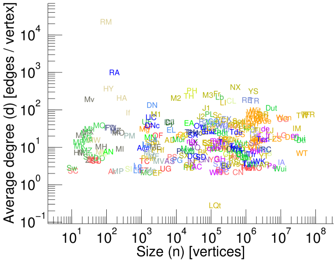
Figure 1: All networks in KONECT arranged by the size (the number of nodes) and the average number of neighbors of all nodes. Each network is represented by a two- or three-character code. The color of each code corresponds to the network category as given in Table 3.

Software and Software Packages

The KONECT project consists of several components, whose interactions is summarized in Figure 2. Various parts of the KONECT project are available at Github, including this Handbook.

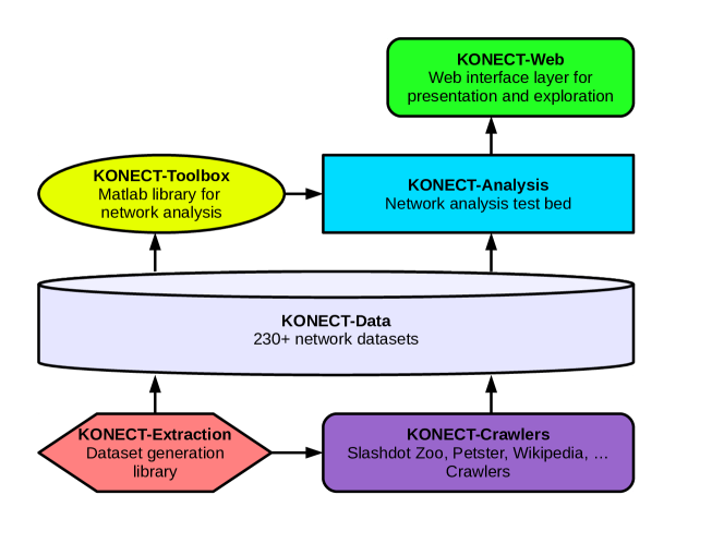
Figure 2: Overview of KONECT’s components.

History of KONECT

KONECT started out in December 2008 at the Technical University of Berlin’s DAI Laboratory, as evaluation for Jérôme Kunegis’s ICML 2009 paper Learning Spectral Graph Transformations for Link Prediction (Kunegis & Lommatzsch, 2009), codenamed Spectral Transformation. It then consisted of a collection of network datasets and spectral link prediction methods. Later, more datasets were added and the codebase was called the Graph Store, and the project was used for the experiments of several papers in the area of collaborative filtering and recommender systems. When Jérôme moved from TU Berlin to the University of Koblenz–Landau in Koblenz (Germany) the project was renamed Web Store, in line with Koblenz’ Institute for Web Science and Technologies (WeST). The name KONECT – Koblenz Network Collection was adopted sometime in 2011. The KONECT website was created in 2011 under konect.uni-koblenz.de. Code for dataset extraction and the Matlab Toolbox was first published on the KONECT website. A short overview paper of the KONECT system was published in 2013 at the International World Wide Web Conference (WWW), as part of the Web Observatory Workshop (Kunegis, 2013). In 2015 and 2016, various parts of KONECT were placed on GitHub under the GNU General Public License version 3, including this handbook. From 2017 on, the KONECT project continued to be developed at the University of Namur (Belgium), with web hosting provided by the Institute for Web Science and Technologies (WeST) at the University of Koblenz–Landau.

Structure of this Handbook

This handbook first describes the different network types covered by KONECT in Section 2, gives important mathematical definitions in Section 3, lists the numerical network statistics in Section 4, lists node features in Section 5, lists the plot types in Section 6, reviews graph characteristic matrices and their decompositions in Section 7, documents the KONECT Toolbox in Section 8 and describes KONECT’s file formats in Section 9. Throughout the handbook, we will use margin notes to give the internal names of various parameters.

2 Networks

Datasets in KONECT represent networks, i.e., a set of nodes connected by links. Networks can be classified by their format (directed/undirected/bipartite), by their edge weight types and multiplicities, by the presence of metadata such as timestamps and node labels, and by the types of objects represented by nodes and links. The full list of networks is given online.

The format of a network is always one of the following. The network formats are summarized in Table 1.

• In undirected networks (U), edges are undirected. That is, there is no difference between the edge from $u$ to $v$ and the edge from $v$ to $u$; both are the edge $\{u,v\}$. An example of an undirected network is the social network of Facebook (Ow), in which there is no difference between the statements “A is a friend of B” and “B is a friend of A.”

• In a directed network (D), the links are directed. That is, there is a difference between the edge $(u,v)$ and the edge $(u,v)$. Directed networks are sometimes also called digraphs (for directed graphs), and their edges arcs. An example of a directed social network is the follower network of Twitter (TF), in which the fact that user A follows user B does not imply that user B follows user A.

• Bipartite networks (B) include two types of nodes, and all edges connect one node type with the other. An example of a bipartite network is a rating graph, consisting of the node types user and movie, and each rating connects a user and a movie (M3). Bipartite networks are always undirected in KONECT.

Table 1: The network formats allowed in KONECT. Each network dataset is exactly of one type.

# Symbol Type Edge partition Edge types Internal name 1 U Undirected Unipartite Undirected sym 2 D Directed Unipartite Directed asym 3 B Bipartite Bipartite Undirected bip

The edge weight and multiplicity types of networks are represented by one of the following eight types. The types of edge weights and multiplicities are summarized in Table 2.

• An unweighted network ($-$) has edges that are unweighted, and only a single edge is allowed between any two nodes.

• In a network with multiple edges ($=$), two nodes can be connected by any number of edges, and all edges are unweighted. This type of network is also called a multigraph.

• In a positive network ($+$), edges are annotated with positive weights, and only a single edge is allowed between any node pair. The weight zero identified with the lack of an edge and thus, we require that each edge has a weight strictly larger than zero.

• In a signed network ($\pm$), both positive and negative edges are allowed. Positive and negative edges are represented by positive and negative edge weights. Many networks of this type have only the weights $\pm 1$, but in the general case we allow any nonzero weight.

• Networks with multiple signed edges ($\stackrel{{\scriptstyle+}}{{=}}$) allow multiple edges between two nodes, which may have the same values as edges in a signed network.

• Rating networks ($*$) have arbitrary real edge weights. They differ from positive and signed networks in that the edge weights are interpreted as an interval scale, and thus the value zero has no special meaning. Adding a constant to all edge weights does not change the semantics of a rating network. Ratings can be discrete, such as the one-to-five star ratings, or continuous, such as a rating given in percent. This type of network allows only a single edge between two nodes.

• Networks with multiple ratings (${}_{*}{}^{*}$) have edges annotated with rating values, and allow multiple edges between two nodes.

• Dynamic networks ($\rightleftarrows$) are networks in which edges can appear and disappear. They are always temporal. Individual edges are not weighted.

Metadata of networks are further properties that go beyond the formats and weights listed above.

• Temporal networks (⏲) include a timestamp for each edge, and thus the network can be reconstructed for any moment in the past.

• Networks with loops ($\circlearrowright$) are unipartite networks in which edges of the form $\{u,u\}$ are allowed, i.e., edges connecting a node with itself.

Table 2: The edge weight and multiplicity types allowed in KONECT. Each network dataset is exactly of one type. Note that due to historical reasons, networks with multiple unweighted edges have the internal name positive, while positively weighted networks have the internal posweighted. For signed networks and positive edge weights, weights of zero are only allowed when the tag #zeroweight is set.

# Symbol Type Multiple Edge weight Edge weight Internal name edges range scale 1 $-$ Unweighted No $\{1\}$ – unweighted 2 $=$ Multiple unweighted Yes $\{1\}$ – positive 3 $+$ Positive weights No $(0,\infty)$ Ratio scale posweighted 4 $\pm$ Signed No $(-\infty,+\infty)$ Ratio scale signed 5 $\stackrel{{\scriptstyle+}}{{=}}$ Multiple signed Yes $(-\infty,+\infty)$ Ratio scale multisigned 6 $*$ Rating No $(-\infty,+\infty)$ Interval scale weighted 7 ${}_{*}{}^{*}$ Multiple ratings Yes $(-\infty,+\infty)$ Interval scale multiweighted 8 $\rightleftarrows$ Dynamic Yes $\{1\}$ – dynamic 9 Multiple positive weights Yes $(0,\infty)$ Ratio scale multiposweighted

Finally, the network categories classify networks by the type of data they represent. An overview of the categories is given in Table 3.

Table 3: The network categories in KONECT. Each category is assigned a color, which is used in plots, for instance in Figure 1. The property symbols are defined in Table 2. U: Undirected network, D: Directed network, B: Bipartite network.

Category Vertices Edges Properties Count $\newmoon$ Affiliation Actors, groups Membership   U D B $-$ $=$ $+$ $\pm$ $\stackrel{{\scriptstyle+}}{{=}}$ $*$ ${}_{*}{}^{*}$ $\rightleftarrows$ $++$ 11 $\newmoon$ Animal Animals Tie   U D B $-$ $=$ $+$ $\pm$ $\stackrel{{\scriptstyle+}}{{=}}$ $*$ ${}_{*}{}^{*}$ $\rightleftarrows$ $++$ 1 $\newmoon$ Authorship Authors, works Authorship   U D B $-$ $=$ $+$ $\pm$ $\stackrel{{\scriptstyle+}}{{=}}$ $*$ ${}_{*}{}^{*}$ $\rightleftarrows$ $++$ 18 $\newmoon$ Citation Documents Citation   U D B $-$ $=$ $+$ $\pm$ $\stackrel{{\scriptstyle+}}{{=}}$ $*$ ${}_{*}{}^{*}$ $\rightleftarrows$ $++$ 6 $\newmoon$ Coauthorship Authors Coauthorship U D B $-$ $=$ $+$ $\pm$ $\stackrel{{\scriptstyle+}}{{=}}$ $*$ ${}_{*}{}^{*}$ $\rightleftarrows$ $++$ 5 $\newmoon$ Communication Persons Message U D B $-$ $=$ $+$ $\pm$ $\stackrel{{\scriptstyle+}}{{=}}$ $*$ ${}_{*}{}^{*}$ $\rightleftarrows$ $++$ 11 $\newmoon$ Computer Computers Connection U D B $-$ $=$ $+$ $\pm$ $\stackrel{{\scriptstyle+}}{{=}}$ $*$ ${}_{*}{}^{*}$ $\rightleftarrows$ $++$ 5 $\newmoon$ Feature Items, features Property   U D B $-$ $=$ $+$ $\pm$ $\stackrel{{\scriptstyle+}}{{=}}$ $*$ ${}_{*}{}^{*}$ $\rightleftarrows$ $++$ 9 $\newmoon$ Folksonomy Users, tags, items Tag assignment   U D B $-$ $=$ $+$ $\pm$ $\stackrel{{\scriptstyle+}}{{=}}$ $*$ ${}_{*}{}^{*}$ $\rightleftarrows$ $++$ 18 $\newmoon$ HumanContact Persons Real-life contact U D B $-$ $=$ $+$ $\pm$ $\stackrel{{\scriptstyle+}}{{=}}$ $*$ ${}_{*}{}^{*}$ $\rightleftarrows$ $++$ 4 $\newmoon$ HumanSocial Persons Real-life tie U D B $-$ $=$ $+$ $\pm$ $\stackrel{{\scriptstyle+}}{{=}}$ $*$ ${}_{*}{}^{*}$ $\rightleftarrows$ $++$ 3 $\newmoon$ Hyperlink Web page Hyperlink   U D B $-$ $=$ $+$ $\pm$ $\stackrel{{\scriptstyle+}}{{=}}$ $*$ ${}_{*}{}^{*}$ $\rightleftarrows$ $++$ 28 $\newmoon$ Infrastructure Location Connection U D B $-$ $=$ $+$ $\pm$ $\stackrel{{\scriptstyle+}}{{=}}$ $*$ ${}_{*}{}^{*}$ $\rightleftarrows$ $++$ 9 $\newmoon$ Interaction Persons, items Interaction   U D B $-$ $=$ $+$ $\pm$ $\stackrel{{\scriptstyle+}}{{=}}$ $*$ ${}_{*}{}^{*}$ $\rightleftarrows$ $++$ 6 $\newmoon$ Lexical Words Lexical relationship U D B $-$ $=$ $+$ $\pm$ $\stackrel{{\scriptstyle+}}{{=}}$ $*$ ${}_{*}{}^{*}$ $\rightleftarrows$ $++$ 6 $\newmoon$ Metabolic Metabolites Interaction U D B $-$ $=$ $+$ $\pm$ $\stackrel{{\scriptstyle+}}{{=}}$ $*$ ${}_{*}{}^{*}$ $\rightleftarrows$ $++$ 6 $\newmoon$ Misc Various Various U D B $-$ $=$ $+$ $\pm$ $\stackrel{{\scriptstyle+}}{{=}}$ $*$ ${}_{*}{}^{*}$ $\rightleftarrows$ $++$ 6 $\newmoon$ OnlineContact Users Online interaction U D B $-$ $=$ $+$ $\pm$ $\stackrel{{\scriptstyle+}}{{=}}$ $*$ ${}_{*}{}^{*}$ $\rightleftarrows$ $++$ 5 $\newmoon$ Rating Users, items Rating   U D B $-$ $=$ $+$ $\pm$ $\stackrel{{\scriptstyle+}}{{=}}$ $*$ ${}_{*}{}^{*}$ $\rightleftarrows$ $++$ 15 $\newmoon$ Social Persons Tie U D B $-$ $=$ $+$ $\pm$ $\stackrel{{\scriptstyle+}}{{=}}$ $*$ ${}_{*}{}^{*}$ $\rightleftarrows$ $++$ 30 $\newmoon$ Software Software Component Dependency   U D B $-$ $=$ $+$ $\pm$ $\stackrel{{\scriptstyle+}}{{=}}$ $*$ ${}_{*}{}^{*}$ $\rightleftarrows$ $++$ 3 $\newmoon$ Text Documents, words Occurrence   U D B $-$ $=$ $+$ $\pm$ $\stackrel{{\scriptstyle+}}{{=}}$ $*$ ${}_{*}{}^{*}$ $\rightleftarrows$ $++$ 5 $\newmoon$ Trophic Species Carbon exchange   U D B $-$ $=$ $+$ $\pm$ $\stackrel{{\scriptstyle+}}{{=}}$ $*$ ${}_{*}{}^{*}$ $\rightleftarrows$ $++$ 3

Affiliation networks

are bipartite networks denoting the membership of actors in groups. Groups can be defined as narrowly as individual online communities in which users have been active (FG) or as broadly as countries (CN). The actors are mainly persons, but can also be other actors such as musical groups. Note that in all affiliation networks we consider, each actor can be in more than one group, as otherwise the network cannot be connected.

Animal networks

are networks of contacts between animals. They are the animal equivalent to human social networks. Note that datasets of websites such as Dogster (Sd) are not included here but in the Social (online social network) category, since the networks are generated by humans.

Authorship networks

are unweighted bipartite networks consisting of links between authors and their works. In some authorship networks such as that of scientific literature (Pa), works have typically only few authors, whereas works in other authorship networks may have many authors, as in Wikipedia articles (en).

Citation networks

consist of documents that reference each other. The primary example are scientific publications, but the category also allow patents and other types of documents that reference each other.

Coauthorship networks

are unipartite network connecting authors ho have written works together, for instance academic literature, but also other types of works such as music or movies.

Communication networks

contain edges that represent individual messages between persons. Communication networks are directed and allow multiple edges. Examples of communication networks are those of emails (EN) and those of Facebook messages (Ow). Note that in some instances, edge directions are not known and KONECT can only provide an undirected network.

Computer networks

are networks of connected computers. Nodes in them are computers, and edges are connections. When speaking about networks in a computer science context, one often means only computer networks. An example is the internet topology network (TO).

Feature networks

are bipartite, and denote any kind of feature assigned to entities. Feature networks are unweighted and have edges that are not annotated with edge creation times. Examples are songs and their genres (GE).

Folksonomies

consist of tag assignments connecting a user, an item and a tag. For folksonomies, we follow the 3-bipartite projection approach and consider the three possible bipartite networks, i.e., the user–item, user–tag and item–tag networks. This allows us to apply methods for bipartite graphs to hypergraphs, which is not possible otherwise. Items that are tagged in folksonomies include bookmarks (Dui), scientific publications (Cui) and movies (Mui).

Human contact networks

are unipartite networks of actual contact between persons, i.e., talking with each other, spending time together, or at least being physically close. Usually, these datasets are collected by giving out RFID tags to people with chips that record which other people are in the vicinity. Determining when an actual contact has happened (as opposed to for instance to persons standing back to back) is a nontrivial research problem. An example is the Reality Mining dataset (RM).

Human social networks

are real-world social networks between humans. The ties must be offline, and not from an online social network. Also, the ties represent a state, as opposed to human contact networks, in which each edge represents an event.

Hyperlink networks

are the networks of web pages connected by hyperlinks.

Infrastructure networks

are networks of physical infrastructure. Examples are road networks (RO), airline connection networks (OF), and power grids (UG).

Interaction networks

are bipartite networks consisting of people and items, where each edge represents an interaction. In interaction networks, we always allow multiple edges between the same person–item pair. Examples are people writing in forums (UF), commenting on movies (Fc), listening to songs (Ls) and sports results.

Lexical networks

consist of words from natural languages and the relationships between them. Relationships can be semantic (i.e, related to the meaning of words) such as the synonym relationship (WO), associative such as when two words are associated with each other by people in experiments (EA), or denote cooccurrence, i.e., the fact that two words co-occur in text (SB). Note that lexical cooccurrence networks are explicitly not included in the broader Cooccurrence category.

Metabolic networks

model metabolic pathways.

Miscellaneous networks

are any networks that do not fit into one of the other categories.

Online Contact networks

consist of people and interactions between them. Contact networks are unipartite and allow multiple edges, i.e., there can always be multiple interactions between the same two persons. They can be both directed or undirected. Examples are people that meet each other (RM), or scientists that write a paper together (Pc).

Physical networks

represent physically existing network structures in the broadest sense. This category covers such diverse data as physical computer networks (TO), transport networks (OF) and biological food networks (FD).

Rating networks

consist of assessments given to items by users, weighted by a rating value. Rating networks are bipartite. Networks in which users can rate other users are not included here, but in the Social category instead. If only a single type of rating is possible, for instance the “favorite” relationship, then rating networks are unweighted. Examples of items that are rated are movies (M3), songs (YS), jokes (JE), and even sexual escorts (SX).

Online social networks

represent ties between persons in online social networking platforms. Certain social networks allow negative edges, which denote enmity, distrust or dislike. Examples are Facebook friendships (FSG), the Twitter follower relationship (TF), and friends and foes on Slashdot (SZ). Note that some social networks can be argued to be rating networks, for instance the user–user rating network of a dating site (LI). These networks are all included in the Social category.

Software networks

are networks of interacting software component. Node can be software packages connected by their dependencies, source files connected by includes, and classes connected by imports.

Text networks

consist of text documents containing words. They are bipartite and their nodes are documents and words. Each edge represents the occurrence of a word in a document. Document types are for instance newspaper articles (TR) and Wikipedia articles (EX).

Trophic networks

consist of biological species connected by edges denotes which pairs of species are subject to carbon exchange, i.e., which species eats which. The term food chain describes such relation ships, but note that in the general case, a trophic network is not a chain, i.e., it is not linear. Trophic networks are directed.

Note that the category system of KONECT is in flux. As networks are added to the collection, large categories are split into smaller ones.

We do not include certain kinds of networks that lack a complex structure. This includes networks without a giant connected component, in which most nodes are not reachable from each other, and trees, in which there is only a single path between any two nodes. Note that bipartite relationships extracted from n-to-1 relationships are therefore excluded, as they lead to a disjoint network. For instance, a bipartite person–city network containing was-born-in edges would not be included, as each city would form its own component disconnected from the rest of the network. On the other hand, a band–country network where edges denote the country of origin of individual band members is included, as members of a single band can have different countries of origin. In fact the Countries network (CN) is of this form. Another example is a bipartite song–genre network, which would only be included in KONECT when songs can have multiple genres. As an example of the lack of complex structure when only a single genre is allowed, the degree distribution in such a song–genre network is skewed because all song nodes have degree one, the diameter cannot be computed since the network is disconnected, and each connected component trivially has a diameter of two or less.

3 Graph Theory

The areas of graph theory and network analysis are young, and many concepts within them notoriously lack a single established notation. The notation chosen for KONECT represents a compromise between familiarity with the most common conventions, and the need to use an unambigous choice of letters and symbols. This section gives an overview of the basic definitions used within KONECT, including in the rest of this handbook.

3.1 Graphs

Graphs will be denoted as $G=(V,E)$, in which $V$ is the set of vertices, and $E$ is the set of edges (Bollobás, 1998). Without loss of generality, we assume that the vertices $V$ are consecutive natural numbers, i.e.,

$$V =\{1,2,3,\dotsc,|V|\}.$$ (1)

Edges $e\in E$ will be denoted as sets of two vertices, i.e., $e=\{u,v\}$. We say that two vertices are adjacent if they are connected by an edge; this will be written as $u\leftrightarrow v$. For directed networks, $u\rightarrow v$ will denote the existence of a directed edge from $u$ to $v$, and $u\rightleftarrows v$ will denote that two directed edges of opposite orientation exist between $u$ and $v$. We say that an edge is incident to a vertex if the edge touches the vertex.

We also allow loops, i.e., edges of the form $\{u,u\}=\{u\}$. Loops appear for instance in email networks, where it is possible to send an email to oneself, and therefore an edge may connect a vertex with itself. Most networks however do not contain loops, and therefore networks that allow loops are annotated in KONECT with the #loop tag, as described in Section 9.

Most of the time, we work with only one given graph, and therefore it is unambigous with node and edge set are meant by $V$ and $E$. When ambiguity is possible, we will however use the notation $V[G]$ and $E[G]$ to denote the vertex and edge sets of a graph $G$. This notation may occasionally be extended to other graph characteristics.

In directed networks, edges are pairs instead of sets, i.e., $e=(u,v)$. In directed networks, edges are sometimes called arcs; in KONECT, we use the term edge for them.

In bipartite graphs, we can partition the set of nodes $V$ into two disjoint sets $V_{1}$ and $V_{2}$, which we will call the left and right set respectively. Although the assignment of a bipartite network’s two node types to left and right sides is mathematically arbitrary, it is chosen in KONECT such that the left nodes are active and the right nodes are passive. For instance, a rating graph with users and items will always have users on the left since they are active in the sense that it is they who give the ratings. Such a distinction is sensible in most networks (Opsahl, 2012). The number of left and right nodes will be denoted $n_{1}=|V_{1}|$ and $n_{2}=|V_{2}|$.

Networks with multiple edges will be written as $G=(V,E)$, where $E$ is a multiset. The degree of nodes in such networks takes into account multiple edges. Thus, the degree does not equal the number of adjacent nodes but the number of incident edges. When $E$ is a multiset, it can contain the edge $\{u,v\}$ multiple times. Mathematically, we may write $\{u,v\}_{1}$, $\{u,v\}_{2}$, etc. Note that we will be lax with this notation. In expressions valid for all types of networks, we will use sums such as $\sum_{\{u,v\}\in E}$ and understand that the sum is over all edges.

In positively weighted networks, we define $w$ as the weight function, returning the edge weight when given an edge. In such networks, the weights are not taken into account when computing the degree.

In a signed network, each edge is assigned a signed weight such as $+1$ or $-1$ (Zaslavsky, 1982). In such networks, we define $w$ to be the signed weight function. In the general case, we allow arbitrary nonzero real numbers, representing degrees of positive and negative edges. Signed relationships have been considered in both phychology (Heider, 1946) and anthropology (Hage & Harary, 1983).

In rating networks, we define $r$ to be the rating function, returning the rating value when given an edge. Note that rating values are interpreted to be invariant under shifts, i.e., adding a real constant to all ratings in the network must not change the semantics of the network. Thus, we will often make use of the mean rating defined as

$$\mu =\frac{1}{|E|}\sum_{e\in E}r(e).$$ (2)

For consistency, we also define the edge weight function $w$ for unweighted and rating networks:

$$w(e) =\left\{\begin{array}[]{ll}1&\text{when $G$ is unweighted}\\ r(e)-\mu&\text{when $G$ is a rating network}\\ \end{array}\right.$$ (5)

We also define a weighting function for node pairs, also denoted $w$. This function takes into account both the weight of edges and edge multiplicities. It is defined as $w(u,v)=0$ when the nodes $u$ and $v$ are not connected and if they are connected as

$$w(u,v) =\left\{\begin{array}[]{ll}1&\text{when $G$ is $-$}\\ |\{k\mid\{u,v\}_{k}\in E\}|&\text{when $G$ is $=$}\\ w(\{u,v\})&\text{when $G$ is $+$}\\ w(\{u,v\})&\text{when $G$ is $\pm$}\\ r(\{u,v\})-\mu&\text{when $G$ is $*$}\\ \sum_{\{u,v\}_{k\in E}}[r(\{u,v\}_{k})-\mu]&\text{when $G$ is ${}_{*}{}^{*}$}\end{array}\right.$$ (12)

Dynamic networks are special in that they have a set of events (edge addition and removal) instead of a set of edges. In most cases, we will model dynamic networks as unweighted networks $G=(V,E)$ representing their state at the latest known timepoint. For analyses that are performed over time, we consider the graph at different time points, with the graph always being an unweighted graph.

In an unweighted graph $G=(V,E)$, the degree of a vertex is the number of neighbors of that node

$$d(u) =\{v\in V\mid\{u,v\}\in E\}.$$ (13)

In networks with multiple edges, the degree takes into account multiple edges, and thus to be precise, it equals the number of incident edges and not the number of adjacent vertices.

$$d(u) =\{\{u,v\}_{k}\in E\mid v\in V\}$$ (14)

In directed graphs, the sum is over all of $u$’s neighbors, regardless of the edge orientation. Note that the sum of the degrees of all nodes always equals twice the number of edges, i.e.,

$$\sum_{v\in V}d(u) =2|E|.$$ (15)

In a directed graph we define the outdegree $d_{1}$ of a node as the number of outgoing edges, and the indegree $d_{2}$ as the number of ingoing edges.

$$d_{1}(u) =\{v\in V\mid(u,v)\in E\}$$ (16)

$$d_{2}(u) =\{v\in V\mid(v,u)\in E\}$$ (17)

The outdegree and indegree are often also denoted $d^{+}(u)$ and $d^{-}(u)$, respectively.

The sum of all outdegrees, and likewise the sum of all indegrees always equals the number of nodes in the network.

$$\sum_{u\in V}d_{1}(u)=\sum_{u\in V}d_{2}(u)=|E|$$ (18)

Thus, the sum of all outdegrees always equals the sum of all indegrees, and therefore the average outdegree always equals the average indegree.

We also define the weight of a node, also denoted by the symbol $w$, as the sum of the absolute weights of incident edges

$$w(u) =\sum_{\{u,v\}\in E}|w(\{u,v\})|.$$ (19)

The weight of a node coincides with the degree of a node in unweighted networks and networks with multiple edges. The weight of a node may also be called its strength (Opsahl et al., 2010).

For directed graphs, we can distinguish the outdegree weight and the indegree weight:

$$w_{\mathrm{O}}(u) =\sum_{(u,v)\in E}|w((u,v))|$$ (20)

$$w_{\mathrm{I}}(u) =\sum_{(v,u)\in E}|w((v,u))|$$ (21)

3.2 Graph Transformations

Sometimes, it is necessary to construct a graph out of another graph. In the following, we briefly review such constructions.

Let $G=(V,E,w)$ be any weighted, signed or rating graph, regardless of edge multiplicities. Then, $\bar{G}$ will denote the corresponding unweighted graph, i.e.,

$$\bar{G} =(V,E).$$ (22)

Note that the graph $\bar{G}$ may still contain multiple edges.

Let $G=(V,E,w)$ be any graph with multiple edges. We define the corresponding unweighted simple graphs as

$$\bar{\bar{G}}=(V,\bar{\bar{E}}),$$ (23)

where $\bar{\bar{E}}$ is the set underlying the multiset $E$. For simple graphs, we define $\bar{\bar{G}}=G$.

Let $G=(V,E,w)$ be a signed or rating network. Then, $|G|$ will denote the corresponding unsigned graph defined by

$$|G| =(V,E,w^{\prime})$$ (24)

$$w^{\prime}(e) =|w(e)|.$$

Let $G=(V,E,w)$ be any network with weight function $w$. The negative network to $G$ is then defined as

$$-G =(V,E,w^{\prime})$$ (25)

$$w^{\prime}(e) =-w(e).$$

This construction is possible for all types of networks. For unweighted and positively weighted networks, it leads to signed networks.

3.3 Algebraic Graph Theory

A very useful representation of graph is using matrices. In fact, a subfield of graph theory, algebraic graph theory, is devoted to this representation (Godsil & Royle, 2001). When a graph is represented as a matrix, operations on graphs can often be expressed as simple algebraic expressions. For instance, the number of common friends of two people in a social network can be expressed as the square of a matrix.

An unweighted graph $G=(V,E)$ can be represented by a $|V|$-by-$|V|$ matrix containing the values 0 and 1, denoting whether a certain edges between two nodes is present. This matrix is called the adjacency matrix of $G$ and will be denoted $\mathbf{A}$. Remember that we assume that the vertices are the natural numbers $1,2,\dotsc,|V|$. Then the entry $\mathbf{A}_{uv}$ is one when $\{u,v\}\in E$ and zero when not. This makes $\mathbf{A}$ square and symmetric for undirected graphs, generally asymmetric (but still square) for directed graphs.

For a bipartite graph $G=(V_{1}\cup V_{2},E)$, the adjacency matrix has the form

$$\mathbf{A} =\left[\begin{array}[]{cc}&\mathbf{B}\\ \mathbf{B}^{\mathrm{T}}&\end{array}\right].$$ (28)

The matrix $\mathbf{B}$ is a $|V_{1}|$-by-$|V_{2}|$ matrix, and thus generally rectangular. $\mathbf{B}$ will be called the biadjacency matrix.

In weighted networks, the adjacency matrix takes into account edge weights. In networks with multiple edges, the adjacency matrix takes into account edge multiplicities. Thus, the general definition of the adjacency matrix is given by

$$\mathbf{A}_{uv} =w(u,v).$$ (29)

The degree matrix $\mathbf{D}$ is a diagonal $|V|$-by-$|V|$ matrix containing the absolute weights of all nodes, i.e.,

$$\mathbf{D}_{uu} =|w(u)|.$$ (30)

Note that we define the degree matrix explicitly to contain node weights instead of degrees, to be consistent with the definition of $\mathbf{A}$.

For directed graphs, we can define the diagonal degree matrix specifically for outdegrees and indegrees as follows:

$$[\mathbf{D}_{\mathrm{O}}]_{uu} =|w_{\mathrm{O}}(u)|$$ (31)

$$[\mathbf{D}_{\mathrm{I}}]_{uu} =|w_{\mathrm{I}}(u)|$$ (32)

The normalized adjacency matrix $\mathbf{N}$ is a $|V|$-by-$|V|$ matrix given by

$$\mathbf{N} =\mathbf{D}^{-1/2}\mathbf{A}\mathbf{D}^{-1/2}.$$ (33)

Finally the Laplacian matrix $\mathbf{L}$ is an $|V|$-by-$|V|$ matrix defined as

$$\mathbf{L}=\mathbf{D}-\mathbf{A}.$$ (34)

Note that in some disciplines the Laplacian matrix may be defined as $\mathbf{A}-\mathbf{D}$, making it negative-semidefinite.

Other matrices used in KONECT include the normalized Laplacian matrix, the stochastic adjacency matrix and the signless Laplacian.

The normalized Laplacian $\mathbf{Z}$ is a normalized version of the Laplacian matrix $\mathbf{L}$. Just as the ordinary Laplacian, $\mathbf{Z}$ capture aspects of the graph that are useful for clustering.

$$\mathbf{Z}=\mathbf{I}-\mathbf{N}=\mathbf{D}^{-1/2}\mathbf{L}\mathbf{D}^{-1/2}$$ (35)

The equation $\mathbf{Z}=\mathbf{I}-\mathbf{N}$ shows that $\mathbf{Z}$ has the same eigenvectors as $\mathbf{N}$, and its eigenvalues are those of $\mathbf{N}$, but shifted and inverted.

The consideration of random walks on a graph leads to the definition of the stochastic adjacency matrix $\mathbf{P}$. Imagine a random walker on the nodes of a graph, who can walk from node to node by following edges. If, at each edge, the probability that the random walker will go to each neighboring node with equal probability, then the random walk can be described be the transition probability matrix defined as

$$\mathbf{P}=\mathbf{D}^{-1}\mathbf{A}=\mathbf{D}^{-1/2}\mathbf{N}\mathbf{D}^{1/2}.$$ (36)

The matrix $\mathbf{P}$ is right stochastic, since its row sums are one.

A further variant of Laplacian matrix is the signless Laplacian $\mathbf{K}$.

$$\mathbf{K}=\mathbf{D}+\mathbf{A}.$$ (37)

The signless Laplacian is also denoted $\mathbf{Q}$. The signless Laplacian $\mathbf{K}$ corresponds to the ordinary Laplacian $\mathbf{L}$ of the graph with inverted edge weights, i.e., $\mathbf{K}[G]=\mathbf{L}[-G]$.

Note that in most cases, we work on just a single graph, and it is implicit that the characteristic matrices apply to this graph. In a few cases, we may need to consider the characteristic matrices of multiple graphs. In these cases, we will write

$$\mathbf{A}[G],\mathbf{D}[G],\mathbf{L}[G],\dotsc$$

to denote the characteristic matrices of the graph $G$.

4 Network Statistics

A network statistic is a numerical value that characterizes a network. Examples of network statistics are the number of nodes and the number of edges in a network, but also more complex measures such as the diameter and the clustering coefficient. Statistics are the basis of most network analysis methods; they can be used to compare networks, classify networks, detect anomalies in networks and for many other tasks. Network statistics are also used to map a network’s structure to a simple numerical space, in which many standard statistical methods can be applied. Thus, network statistics are essential for the analysis of almost all network types. All statistics described in KONECT are real numbers.

This section gives the definitions for the statistics supported by KONECT, and briefly reviews their uses. All network statistics can be computed using the KONECT Toolbox using the function konect_statistic(). Each statistic has an internal name that must be passed as the first argument to konect_statistic(). The internal names are given in the margin in this section. Additionally, the KONECT Toolbox includes functions named konect_statistic_<NAME>() which compute a single statistic <NAME>.

The values of selected statistics are shown for the KONECT networks on the website.

4.1 Basic Network Statistics

Some statistics are simple to define, trivial to compute, and are reported universally in studies about networks. These include the number of nodes, the number of edges, and statistics derived from them such as the average number of neighbors a node has.

The size of a network is the number of nodes it contains, and is almost universally denoted $n$. The size of a graph is sometimes also called the order of the graph.

$$\marginpar{\normalcolor\raggedright\texttt{size}}n\@add@raggedright =|V|$$ (38)

In a bipartite graph, the size can be decomposed as $n=n_{1}+n_{2}$ with $n_{1}=|V_{1}|$ and $n_{2}=|V_{2}|$. The size of a network is not necessarily a very meaningful number. For instance, adding a node without edges to a network will increase the size of the network, but will not change anything in the network. In the case of an online social network, this would correspond to creating a user account and not connecting it to any other users – this adds an inactive user, which are often not taken into account. Therefore, a more representative measure of the size of a network is actually given by the number of edges, giving the volume of a network.

The volume of a network equals the number of edges and is defined as

$$\marginpar{\normalcolor\raggedright\texttt{volume}}m\@add@raggedright =|E|.$$ (39)

Note that in mathematical contexts, the number of edges may be called the size of the graph, in which case the number of nodes is called the order. In this text, we will consistently use size for the number of nodes and volume for the number of edges.

The volume can be expressed in terms of the adjacency or biadjacency matrix of the underlying unweighted graph as

$$m =\left\{\begin{array}[]{ll}\frac{1}{2}\|\mathbf{A}[\bar{G}]\|_{\mathrm{F}}^{2}&\text{when $G$ is undirected}\\ \|\mathbf{A}[\bar{G}]\|_{\mathrm{F}}^{2}&\text{when $G$ is directed}\\ \|\mathbf{B}[\bar{G}]\|_{\mathrm{F}}^{2}&\text{when $G$ is bipartite}\end{array}\right.$$ (43)

The number of edges in network is often considered a better measure of the size of a network than the number vertices, since a vertex unconnected to any other vertices may often be ignored. On the practical side, the volume is also a much better indicator of the amount of memory needed to represent a network.

We will also make use of the number of edges without counting multiple edges. We will call this the unique volume of the graph.

$$\marginpar{\normalcolor\raggedright\texttt{uniquevolume}}\bar{\bar{m}}\@add@raggedright =m[\bar{\bar{G}}]$$ (44)

The weight $w$ of a network is defined as the sum of absolute edge weights. For unweighted networks, the weight equals the volume. For rating networks, remember that the weight is defined as the sum over ratings from which the overall mean rating has been subtracted, in accordance with the definition of the adjacency matrix for these networks.

$$\marginpar{\normalcolor\raggedright\texttt{weight}}w\@add@raggedright =\sum_{e\in E}|w(e)|$$ (45)

The average degree is defined as

$$\marginpar{\normalcolor\raggedright\texttt{avgdegree}}d\@add@raggedright =\frac{1}{|V|}\sum_{u\in V}d(u)=\frac{2m}{n}.$$ (46)

The average degree is sometimes called the density. We avoid the term density in KONECT as it is sometimes used for the fill, which denotes the probability that an edge exists. In bipartite networks, we additionally define the left and right average degree

$$d_{1} =\frac{1}{|V_{1}|}\sum_{u\in V_{1}}d(u)=\frac{m}{n_{1}}$$ (47)

$$d_{2} =\frac{1}{|V_{2}|}\sum_{u\in V_{2}}d(u)=\frac{m}{n_{2}}$$ (48)

Note that in directed networks, the average outdegree equals the average indegree, and both are equal to $m/n$.

The fill of a network is the proportion of edges to the total number of possible edges. The fill is used as a basic parameter in the Erdős–Rényi random graph model (Erdős & Rényi, 1959), where it denotes the probability that an edge is present between two randomly chosen nodes, and is usually called $p$, which is the notation we also use in KONECT.

$$\marginpar{\normalcolor\raggedright\texttt{fill}}p\@add@raggedright =\left\{\begin{array}[]{ll}2m/[n(n-1)]&\text{when $G$ is undirected without loop}\\ 2m/[n(n+1)]&\text{when $G$ is undirected with loops}\\ m/[n(n-1)]&\text{when $G$ is directed without loops}\\ m/n^{2}&\text{when $G$ is directed with loops}\\ m/(n_{1}n_{2})&\text{when $G$ is bipartite}\end{array}\right.$$ (54)

In the undirected case, the expression is explained by the fact that the total number of possible edges is $n(n-1)/2$ excluding loops. The fill is sometimes also called the density of the network, in particular in a mathematical context, or the connectance of the network.

The maximum degree equals the highest degree value attained by any node.

$$\marginpar{\normalcolor\raggedright\texttt{maxdegree}}d_{\max}\@add@raggedright =\max_{u\in V}d(u)$$ (55)

The maximum degree can be divided by the average degree to normalize it.

$$\marginpar{\normalcolor\raggedright\texttt{relmaxdegree}}d_{\mathrm{MR}}\@add@raggedright =\frac{d_{\max}}{d}$$ (56)

In a directed network, the reciprocity equals the proportion of edges for which an edge in the opposite direction exists, i.e., that are reciprocated (Garlaschelli & Loffredo, 2004).

$$\marginpar{\normalcolor\raggedright\texttt{reciprocity}}y=\frac{1}{m}|\{(u,v)\in E\mid(v,u)\in E\}|\@add@raggedright$$ (57)

The reciprocity has also been noted $r$ (Szell et al., 2010). The reciprocity can give an idea of the type of network. For instance, citation networks only contain only few pairs of papers that mutually cite each other. On the other hand, an email network will contain many pairs of people who have sent emails to each other. Thus, citation networks typically have low reciprocity, and communnication networks have high reciprocity.

4.2 Connectivity Statistics

Connectivity statistics measure to what extent a network is connected. Two nodes are said to be connected when they are either directly connected through an edge, or indirectly through a path of several edges. A connected component is a set of vertices all of which are connected, and unconnected to the other nodes in the network. The largest connected component in a network is usually very large and called the giant connected component. When it contains all nodes, the network is connected.

The size of the largest connected component is denoted $N$.

$$\marginpar{\normalcolor\raggedright\texttt{coco}}N\@add@raggedright =\max_{F\subseteq\mathcal{C}}|F|$$ (58)

$$\mathcal{C} =\{C\subseteq V\mid\forall u,v\in C:\exists w_{1},w_{2},\ldots\in V:u\leftrightarrow w_{1}\leftrightarrow w_{2}\leftrightarrow\cdots\leftrightarrow v\}$$

In bipartite networks, the number of left and right nodes in the largest connected components are denoted $N_{1}$ and $N_{2}$, with $N_{1}+N_{2}=N$.

The relative size of the largest connected component equals the size of the largest connected component divided by the size of the network

$$\marginpar{\normalcolor\raggedright\texttt{cocorel}}N_{\mathrm{rel}}\@add@raggedright =\frac{N}{n}.$$ (59)

We also use an inverted variant of the relative size of the largest connected component, which makes it easier to plot the values of a logarithmic scale.

$$\marginpar{\normalcolor\raggedright\texttt{cocorelinv}}N_{\mathrm{inv}}\@add@raggedright =1-\frac{N}{n}$$ (60)

In directed networks, we additionally define the size of the largest strongly connected component $N_{\mathrm{s}}$. A strongly connected component is a set of vertices in a directed graph such that any node is reachable from any other node using a path following only directed edges in the forward direction. We always have $N_{\mathrm{s}}\leq N$.

4.3 Subgraph Count Statistics

Figure 3: A 2-star is a graph consisting of three nodes, two of which are connected. 2-stars are occasionally called cherries due to their resemblance to the fruit.

The fundamental building block of a network are the edges. Thus, the number of edges is a basic statistic of any network. To understand the structure of a network, it is however not enough to analyse edges individually. Instead, larger patterns such as triangles must be considered. These patterns can be counted, and give rise to count statistics, i.e., statistics that count the number of ocurrences of specific patterns.

Table 4 gives a list of fundamental patterns in networks, and their corresponding count statistics.

Table 4: Subgraph patterns that occur in networks. Each pattern can be counted, giving rise to a count statistic.

Pattern Name(s) Statistic Internal name Node, 0-star, 0-path, 1-clique $n$ size Edge, 1-star, 1-path, 2-clique $m$ volume Wedge, 2-star, 2-path $s$ twostars Triangle, 3-cycle, 3-clique $t$ triangles Claw, 3-star $z$ threestars Square, 4-cycle $q$ squares Cross, 4-star $x$ fourstars $k$-Star $S_{k}$ $k$-Path $P_{k}$ $k$-Cycle $C_{k}$ $k$-Clique $K_{k}$

A star is defined as a graph in which a central node is connected to all other nodes, and no other edges are present. Specifically, a $k$-star is defined as a star in which the central node is connected to $k$ other nodes. Thus, a 2-star consists of a node connected to two other nodes, or equivalently two incident edges, or a path of length 2. The specific name for 2-stars is wedges. The number of wedges can be defined as

$$\marginpar{\normalcolor\raggedright\texttt{twostars}}s=\sum_{u\in V}{d(u)\choose 2}=\sum_{u\in V}\frac{1}{2}d(u)(d(u)-1),\@add@raggedright$$ (61)

where $d(u)$ is the degree of node $u$. Wedges have many different names: 2-stars, 2-paths, hairpins (e.g. Gleich & Owen, 2012) and cherries.

Three-stars are defined analogously to two-stars, and their count denoted $z$. Three-stars are also called claws and tripins (e.g. Gleich & Owen, 2012).

$$\marginpar{\normalcolor\raggedright\texttt{threestars}}z=\sum_{u\in V}{d(u)\choose 3}=\sum_{u\in V}\frac{1}{6}d(u)(d(u)-1)(d(u)-2)\@add@raggedright$$ (62)

In the general case, the number of $k$-stars is defined as

$$S_{k} =\sum_{u\in V}{d(u)\choose k}$$ (63)

The number of triangles defined in the following way is independent of the orientation of edges when the graph is directed. Loops in the graph, as well as edge multiplicities, are ignored.

$$\marginpar{\normalcolor\raggedright\texttt{triangles}}t=|\{\{u,v,w\}\mid u\leftrightarrow v\leftrightarrow w\leftrightarrow u\}|\;/\;6\@add@raggedright$$ (64)

A square is a cycle of length four, and the number of squares in a graph is denoted $q$.

$$\marginpar{\normalcolor\raggedright\texttt{squares}}q=|\{u,v,w,x\mid u\leftrightarrow v\leftrightarrow w\leftrightarrow x\leftrightarrow u\}|\;/\;8\@add@raggedright$$ (65)

The factor 8 ensures that squares are counted regardless of their edge labeling.

Multiple edges are ignored in these count statistics, and edges in patterns are not allowed to overlap.

Triangles and squares are both cycles – which we can generalize to $k$-cycles, sequences of $k$ distinct vertices that are cyclically linked by edges. We denote the number of $k$-cycles by $C_{k}$. For small $k$, we note the following equivalences:

$$C_{1} =0$$

$$C_{2} =m$$

$$C_{3} =t$$

$$C_{4} =q$$

for graphs without loops. Cycles of length three and four have special notation: $C_{3}=t$ and $C_{4}=q$ and are called triangles and squares.

A cycle cannot the same node twice. Due to this combinatorial restriction, $C_{k}$ is quite complex to compute for large $k$. Therefore, we may use tours instead, defined as cyclical lists of connected vertices in which we allow several vertices to overlap. The number of $k$-tours will be denoted $T_{k}$. For computational conveniance, we will define labeled tours, where two tours are not equal when they are identical up to shifts or inversions. We note the following equalities:

$$T_{1} =0$$

$$T_{2} =2m$$

$$T_{3} =6t$$

$$\marginpar{\normalcolor\raggedright\texttt{tour4}}T_{4}\@add@raggedright =8q+4s+2m$$ (66)

Again, these are true when the graph is loopless. The last equality shows that trying to divide the tour count by $2k$ to count them up to shifts and inversions is a bad idea, since it cannot be implemented by dividing the present definition by $2k$.

As mentioned before, counting cycles is a complex problem. Counting tours is however much easier. The number of tours of length $k$ can be expressed as the trace of a power of the graph’s adjacency matrix, and thus also as a moment of the adjacency matrix’s spectrum when $k>2$.

$$T_{k} =\mathrm{Tr}(\mathbf{A}^{k})=\sum_{i}\lambda_{i}[\mathbf{A}]^{k}$$

This remains true when the graph includes loops.

4.4 Degree Distribution Statistics

The distribution of degree values $d(u)$ over all nodes $u$ is often taken to characterize a network. Thus, a certain number of network statistics are based solely on this distribution, regardless of overall network structure.

The power law exponent is a number that characterizes the degrees of the nodes in the network. In many circumstances, networks are modeled to follow a degree distribution power law, i.e., the number of nodes with degree $n$ is taken to be proportional to the power $n^{-\gamma}$, for a constant $\gamma$ larger than one (Barabási & Albert, 1999). This constant $\gamma$ is called the power law exponent. Given a network, its degree distribution can be used to estimate a value $\gamma$. There are multiple ways of estimating $\gamma$, and thus a network does not have a single definite value of it. In KONECT, we estimate $\gamma$ using the robust method given in (Newman, 2006, Eq. 5)

$$\marginpar{\normalcolor\raggedright\texttt{power}}\gamma\@add@raggedright =1+n\left(\sum_{u\in V}\ln\frac{d(u)}{d_{\min}}\right)^{-1},$$ (67)

in which $d_{\min}$ is the minimal degree.

The Gini coefficient is a measure of inequality from economics, typically applied to distributions of wealth or income. In KONECT, we apply it to the degree distribution, as described in (Kunegis & Preusse, 2012). The Gini coefficient can either be defined in terms of the Lorenz curve, a type of plot that visualizes the inequality of a distribution, or using the following expression. Let $d_{1}\leq d_{2}\leq\dotsb\leq d_{n}$ be the sorted list of degrees in the network. Then, the Gini coefficient is defined as

$$\marginpar{\normalcolor\raggedright\texttt{gini}}G\@add@raggedright =\frac{2\sum_{i=1}^{n}id_{i}}{n\sum_{i-1}^{n}d_{i}}-\frac{n+1}{n}.$$ (68)

The Gini coefficient takes values between zero and one, with zero denoting total equality between degrees, and one denoting the dominance of a single node.

The relative edge distribution entropy is a measure of the equality of the degree distribution, and equals one when all degrees are equal, and attains the limit value of zero when all edges attach to a single node (Kunegis & Preusse, 2012). It is defined as

$$\marginpar{\normalcolor\raggedright\texttt{dentropyn}}H_{\mathrm{er}}\@add@raggedright =\frac{1}{\ln n}\sum_{u\in V}-\frac{d(u)}{2m}\ln\frac{d(u)}{2m}.$$ (69)

Another statistic for measuring the inequality in the degree distribution is associated with the Lorenz curve (see Section 6.4), and is given by the intersection point of the Lorenz curve with the antidiagonal given by $y=1-x$ (Kunegis & Preusse, 2012). By construction, this point equals $(1-P,P)$ for some $0<P<1$, where the value $P$ corresponds exactly to the number “25%” in the statement “25% of all users account for 75% of all friendship links on Facebook”. By construction, we can expect $P$ to be smaller when $G$ is large.

The analysis of degrees can be generalized to pairs of nodes: What is the distribution of degrees for pairs of connected edges? In some networks, high-degree nodes are connected to other high-degree nodes, while low-degree nodes are connected to low-degree nodes. This property is called assortativity (Newman, 2003a). Inversely, in a network with dissortativity, high-degree nodes are typically connected to low-degree and vice versa. The amount of assortativity can be measured by the Pearson correlation $\rho$ between the degree of connected nodes.

$$\marginpar{\normalcolor\raggedright\texttt{\smallassortativity}}\rho\@add@raggedright =\frac{\sum_{\{u,v\}\in E}(d(u)-d)(d(v)-d)}{\sum_{\{u,v\}\in E}(d(u)-d)^{2}}$$ (70)

The assortativity is undefined whenever the Pearson correlation is undefined, for instance, if all nodes have the same degree (i.e., when the graph is regular), and when the graph does not contain any edges.

4.5 Clustering Statistics

The term clustering refers to the observation that in almost all networks, nodes tend to form small groups within which many edges are present, and such that only few edges connected different clusters with each other. In a social network for instance, people form groups in which almost every member known the other members. Clustering thus forms one of the primary characteristics of real-world networks, and thus many statistics for measuring it have been defined. The main method for measuring clustering numerically is the clustering coefficient, of which there exist several variants. As a general rule, the clustering coefficient measures to what extent edges in a network tend to form triangles. Since it is based on triangles, it can only be applied to unipartite networks, because bipartite networks do not contain triangles.

The number of triangles $t$ itself as defined in Section 4.3 is however not a statistic that can be used to measure the clustering in a network, since it correlates with the size and volume of the network. Instead, the clustering coefficients in all its variants can be understood as a count of triangles, normalized in different ways in order to compare several networks with it.

The local clustering coefficient $c(u)$ of a node $u$ is defined as the probability that two randomly chosen (but distinct) neighbors of $u$ are connected (Watts & Strogatz, 1998).

$$c(u) =\left\{\begin{array}[]{ll}\frac{\{v,w\in V\mid u\leftrightarrow v\leftrightarrow w\leftrightarrow u\}}{\{v,w\in V\mid u\leftrightarrow v\neq w\leftrightarrow u\}}&\text{when }d(u)>1\\ 0&\text{when }d(u)\leq 1\end{array}\right.$$ (73)

The global clustering of a network can be computed in two ways. The first way defines it as the probability that two incident edges are completed by a third edge to form a triangle (Newman et al., 2002). This is also called the transitivity ratio, or simply the transitivity.

$$\marginpar{\normalcolor\raggedright\texttt{clusco}}c\@add@raggedright =\frac{|\{u,v,w\in V\mid u\leftrightarrow v\leftrightarrow w\leftrightarrow u\}|}{|\{u,v,w\in V\mid u\leftrightarrow v\neq w\leftrightarrow u\}|}=\frac{3t}{s}$$ (74)

This variant of the global clustering coefficient has values between zero and one, with a value of one denoting that all possible triangles are formed (i.e., the network consists of disconnected cliques), and zero when it is triangle free. Note that the clustering coefficient is trivially zero for bipartite graphs. This clustering coefficient is however not defined when each node has degree zero or one, i.e., when the graph is a disjoint union of edges and unconnected nodes. This is however not a problem in practice.

The second variant variant of the clustering coefficient uses the average of the local clustering coefficients. This second variant was historically the first to be defined. In was defined in 1998 (Watts & Strogatz, 1998) and precedes the first variant by four years.

$$\marginpar{\normalcolor\raggedright\texttt{clusco2}}c_{2}\@add@raggedright =\frac{1}{|V|}\sum_{u\in V}c(u)$$ (75)

This second variant of the global clustering coefficient is zero when a graph is triangle-free, and one when the graph is a disjoint union of cliques of size at least three. This variant of the global clustering coefficient is defined for all graphs, except for the empty graph, i.e., the graph with zero nodes. A slightly different definition of the second variant computes the average only over nodes with a degree of at least two, as seen for instance in (Bansal et al., 2008).

Because of the arbitrary decision to define $c(u)$ as zero when the degree of $c$ is zero or one, we recommend to use the first variant of the clustering coefficient. In the following, the extensions to the clustering coefficient we present are all based on the first variant, $c$.

For signed graphs, we may define the clustering coefficient to take into account the sign of edges. The signed clustering coefficient is based on balance theory (Kunegis et al., 2009). In a signed network, edges can be positive or negative. For instance in a signed social network, positive edges represent friendship, while negative edges represent enmity. In such networks, balance theory stipulates than triangles tend to be balanced, i.e., that three people are either all friends, or two of them are friends with each other, and enemies with the third. On the other hand, a triangle with two positive and one negative edge, or a triangle with three negative edges is unbalanced. In other words, we can define the sign of a triangle as the product of the three edge signs, which then leads to the stipulation that triangles tend to have positive weight. To extend the clustering coefficient to signed networks, we thus distinguis between balanced and unbalanced triangles, in a way that positive triangles contribute positively to the signed clustering coefficient, and negative triangles contribute negatively to it. For a triangle $\{u,v,w\}$, let $\sigma(u,v,w)=w(u,v)w(v,w)w(w,u)$ be the sign of the triangle, then the following definition captures the idea:

$$c_{\mathrm{s}} =\frac{\sum_{u,v,w\in V}\sigma(u,v,w)}{|\{u,v,w\in V\mid u\leftrightarrow v\neq w\leftrightarrow u\}|}$$ (76)

Here, the sum is over all triangles $\{u,v,w\}$, but can also be taken over all triples of vertices, since $w(u,v)=0$ when $\{u,v\}$ is not an edge.

The signed clustering coefficient is bounded by the clustering coefficient:

$$|c_{\mathrm{s}}|\leq c$$ (77)

The relative signed clustering coefficient can then be defined as

$$c_{\mathrm{r}}=\frac{c_{\mathrm{s}}}{c}=\frac{\sum_{u,v,w\in V}\sigma(u,v,w)}{|\{u,v,w\in V\mid u\leftrightarrow v\leftrightarrow w\leftrightarrow u\}|}$$ (78)

which also equals the proportion of all triangles that are balanced, minus the proportion of edges that are unbalanced.

4.6 Distance Statistics

The distance between two nodes in a network is defined as the number of edges needed to reach one node from another, and serves as the basis for a class of network statistics.

A path in a network is a sequence of incident edges, or equivalently, a sequence of nodes $P=(u_{0},u_{2},\dotsc,u_{k})$, such that $(u_{i},u_{i+1})\in E$ for all $i\in\{0,\dotsc,k-1\}$. The number $k$ is called the length of the path, and will also be denoted $l(P)$. A further restriction can be set on the visited nodes, definining that each node can only be visited at most once. If the distinction is made, the term path is usually reserved for sequences of non-repeating nodes, and general sequence of adjacent nodes are then called walks. We will not make this distinction here.

Paths in networks can be used to model browsing behavior of people in hyperlink networks, navigation in transport networks, and other types of movement-like activities in a network. When considering navigation and browsing, an important problem is the search for shortest paths. Since the length of a path determines the number of steps needed to reach one node from another, it can be used as a measure of distance between nodes of a network. The distance defined in this way may also be called the shortest-path distance to distinguish it from other distance measures between nodes of a network.

$$d(u,v) =\left\{\begin{array}[]{ll}\min_{P=(u,\dotsc,v)}l(P)&\text{when $u$ and $v$ are connected}\\ \infty&\text{when $u$ and $v$ are not connected}\end{array}\right.$$ (81)

In the case that a network is not connected, the distance is defined as infinite. In practice, only the largest connected component of a network may be used, making it unnecessary to deal with infinite values. The distribution of all $|V|^{2}$ values $d(u,v)$ for all $u,v\in V$ is called the distance distribution, and it too characterizes the network.

The eccentricity of a node can then be defined as the maximal distance from that node to any other node, defining a measure of non-centrality:

$$\epsilon(u) =\max_{v\in V}d(u,v)$$ (82)

The diameter $\delta$ of a graph equals the longest shortest path in the network (Newman, 2003b). It can be equivalently defined as the largest eccentricity of all nodes.

$$\marginpar{\normalcolor\raggedright\texttt{diam}}\delta\@add@raggedright =\max_{u\in V}\epsilon(u)=\max_{u,v\in V}d(u,v)$$ (83)

Note that the diameter is undefined (or infinite) in unconnected networks, and thus in numbers reported for actual networks in KONECT we consider always the diameter of the network’s largest connected component. Du to the high runtime complexity of computing the diameter, it may be estimated by various methods, in which case it is noted noted $\tilde{\delta}$.

A statistic related to the diameter is the radius, defined as the smallest eccentricity

$$\marginpar{\normalcolor\raggedright\texttt{radius}}r\@add@raggedright =\min_{u\in V}\epsilon(u)=\min_{u\in V}\max_{v\in V}d(u,v)$$ (84)

The diameter is bounded from below by the radius, and from above by twice the radius.

$$r\leq\delta\leq 2r$$

The first inequality follows directly from the definitions of $r$ and $\delta$ as the minimal and maximal eccentricity. The second inequality follows from the fact that between any two nodes, the path joining them cannot be longer that the path joining them going through a node with minimal eccentricity, which has length of at most $2r$.

The radius and the diameter are not very expressive statistics: Adding or removing an edge will, in many cases, not change their values. Thus, a better statistic that reflects the typical distances in a network in given by the mean and average distance.

The mean path length $\delta_{\mathrm{m}}$ in a network is defined as as the mean distance over all node pairs, including the distance between a node and itself:

$$\marginpar{\normalcolor\raggedright\texttt{meandist}}\delta_{\mathrm{m}}\@add@raggedright =\frac{1}{n^{2}}\sum_{u\in V}\sum_{v\in V}d(u,v)$$ (85)

The mean path length defined in this way is undefined when a graph is disconnected. Also, the average inverse distance has been used, or equivalently, the inverse of the harmonic mean of distances (Latora & Marchiori, 2001).

Likewise, the median path length $\delta_{\mathrm{M}}$ is the median length of shortest paths in the network. In KONECT, both the median and mean path lengths are computed taking into account node pairs of the form $(u,u)$.

Both the mean and median path length can be called the characteristic path length of the network.

A related statistic is the 90-percentile effective diameter $\delta_{0.9}$, which equals the number of edges needed on average to reach 90% of all other nodes.

4.7 Algebraic Statistics

Algebraic statistics are based on a network’s characteristic matrices. They are motivated by the broader field of spectral graph theory, which characterizes graphs using the spectra of these matrices (Chung, 1997).

In the following we will denote by $\lambda_{k}[\mathbf{X}]$ the $k$^th dominant eigenvalue of the matrix $\mathbf{X}$. For the adjacency matrix $\mathbf{A}$, the dominant eigenvalues are the largest absolute ones; for the Laplacian $\mathbf{L}$ they are the smallest ones.

Also, the matrix $\mathbf{L}$ will only be considered for the network’s largest connected component.

The spectral norm of a network equals the spectral norm (i.e., the largest absolute eigenvalue) of the network’s adjacency matrix

$$\marginpar{\normalcolor\raggedright\texttt{snorm}}\left\|\mathbf{A}\right\|_{2}\@add@raggedright =|\lambda_{1}[\mathbf{A}]|.$$ (86)

The spectral norm can be understood as an alternative measure of the size of a network.

The algebraic connectivity equals the second smallest nonzero eigenvalue of $\mathbf{L}$ (Fiedler, 1973)

$$\marginpar{\normalcolor\raggedright\texttt{alcon}}a\@add@raggedright =\lambda_{2}[\mathbf{L}].$$ (87)

The algebraic connectivity is zero when the network is disconnected – this is one reason why we restrict the matrix $\mathbf{L}$ to each network’s giant connected component. The algebraic connectivity is larger the better the network’s largest connected component is connected.

In signed and ratings networks, i.e., networks in which the weights of node pairs can be negative, the smallest eigenvalue of $\mathbf{L}$ can be larger than zero. (In other networks, it is always zero.) The algebraic conflict equals this smallest eigenvalue

$$\marginpar{\normalcolor\raggedright\texttt{conflict}}\xi\@add@raggedright =\lambda_{1}[\mathbf{L}].$$ (88)

The algebraic conflict measures the amount of conflict in the network, i.e., the tendency of the network to contain cycles with an odd number of negatively weighted edges.

4.8 Bipartivity Statistics

Some unipartite networks are almost bipartite. Almost-bipartite networks include networks of sexual contact (Liljeros et al., 2001) and ratings in online dating sites (Brožovský & Petříček, 2007; Kunegis et al., 2012). Other, more subtle cases, involve online social networks. For instance, the follower graph of the microblogging service Twitter is by construction unipartite, but has been observed to reflect, to a large extent, the usage of Twitter as a news service (Kwak et al., 2010). This is reflected in the fact that it is possible to indentify two kinds of users: Those who primarily get followed and those who primarily follow. Thus, the Twitter follower graph is almost bipartite. Other social networks do not necessarily have a near-bipartite structure, but the question might be interesting to ask to what extent a network is bipartite. To answer this question, measures of bipartivity have been developed.

Instead of defining measures of bipartivity, we will instead consider measures of non-bipartivity, as these can be defined in a way that they equal zero when the graph is bipartite. Given an (a priori) unipartite graph, a measure of non-bipartivity characterizes the extent to which it fails to be bipartite. These measures are defined for all networks, but are trivially zero for bipartite networks. For non-bipartite networks, they are larger than zero.

A first measure of bipartivity consists in counting the minimum number of frustrated edges (Holme et al., 2003). Given a bipartition of vertices $V=V_{1}\cup V_{2}$, a frustrated edge is an edge connecting two nodes in $V_{1}$ or two nodes in $V_{2}$. Let $f$ be the minimal number of frustrated edges in any bipartition of $V$, or, put differently, the minimum number of edges that have to be removed from the graph to make it bipartite. Then, a measure of non-bipartivity is given by

$$\marginpar{\normalcolor\raggedright\texttt{frustration}}F\@add@raggedright =\frac{f}{|E|}.$$ (89)

This statistic is always in the range $[0,1/2]$. It attains the value zero if and only if $G$ is bipartite.

The minimal number of frustrated edges $f$ can be approximated by algebraic graph theory. First, we represent a bipartition $V=V_{1}\cup V_{2}$ by its characteristic vector $\mathbf{x}\in\mathbb{R}^{|V|}$ defined as

$$\mathbf{x}_{u} =\left\{\begin{array}[]{ll}+1/2&\text{when $u\in V_{1}$}\\ -1/2&\text{when $u\in V_{2}$}\end{array}\right.$$

Note that the number of edges connecting the sets $V_{1}$ and $V_{2}$ is then given by

$$\left\{\{u,v\}\mid u\in V_{1},v\in V_{2}\right\}=\frac{1}{2}\mathbf{x}^{\mathrm{T}}\mathbf{K}[\bar{G}]\mathbf{x} =\frac{1}{2}\sum_{(u,v)\in E}(\mathbf{x}_{u}+\mathbf{x}_{v})^{2},$$

where $\mathbf{K}[\bar{G}]=\mathbf{D}[\bar{G}]+\mathbf{A}[\bar{G}]$ is the signless Laplacian matrix of the underlying unweighted graph. Thus, the minimal number of frustrated edges $f$ is given by

$$f =\min_{\mathbf{x}\in\{\pm 1/2\}^{|V|}}\frac{1}{2}\mathbf{x}^{\mathrm{T}}\mathbf{K}[\bar{G}]\mathbf{x}.$$

By relaxing the condition $\mathbf{x}\in\{\pm 1/2\}^{|V|}$, we can express $f$ in function of $\mathbf{K}[\bar{G}]$’s minimal eigenvalue, using the fact that the norm of all vectors $\mathbf{x}\in\{\pm 1/2\}^{|V|}$ equals $\sqrt{|V|/4}$, and the property that the minimal eigenvalue of a matrix equals its minimal Rayleigh quotient.

$$\frac{2f}{|V|/4} \approx\min_{\mathbf{x}\neq\mathbf{0}}\frac{\mathbf{x}^{\mathrm{T}}\mathbf{K}[\bar{G}]\mathbf{x}}{\left\|\mathbf{x}\right\|^{2}}=\lambda_{\min}[\mathbf{K}[\bar{G}]]$$

We can thus approximate the previous measure of non-bipartivity by

$$\marginpar{\normalcolor\raggedright\texttt{anticonflict}}\tilde{F}\@add@raggedright =\frac{|V|}{8|E[\bar{G}]|}\lambda_{\min}[\mathbf{K}[\bar{G}]]$$ (90)

The eigenvalue $\lambda_{\min}[\mathbf{K}[\bar{G}]]$ can also be interpreted as the algebraic conflict in $G$ interpreted as a signed graph in which all edges have negative weight.

A further measure of bipartivity exploits the fact that the adjacency matrix $\mathbf{A}$ of a bipartite graph has eigenvalues symmetric around zero, i.e., all eigenvalues of a bipartite graph come in pairs $\pm\lambda$. Thus, the ratio of the smallest and largest eigenvalues can be used as a measure of non-bipartivity

$$\marginpar{\normalcolor\raggedright\texttt{nonbip}}b_{\mathrm{A}}\@add@raggedright =1-\left|\frac{\lambda_{\min}[\mathbf{A}[\bar{G}]]}{\lambda_{\max}[\mathbf{A}[\bar{G}]]}\right|,$$ (91)

where $\lambda_{\min}$ and $\lambda_{\max}$ are the smallest and largest eigenvalue of the given matrix, and $\bar{G}$ is the unweighted graph underlying $G$. Since the largest eigenvalue always has a larger absolute value than the smallest eigenvalue (due to the Perron–Frobenius theorem, and from the nonnegativity of $\mathbf{A}[\bar{G}]$), it follows that this measure of non-bipartivity is always in the interval $[0,1)$, with zero denoting a bipartite network.

Another spectral measure of non-bipartivity is based on considering the smallest eigenvalue of the matrix $\mathbf{N}[\bar{G}]$. This eigenvalue is $-1$ exactly when $G$ is bipartite. Thus, this value minus one is a measure of non-bipartivity. Equivalently, it equals two minus the largest eigenvalue of the normalized Laplacian matrix $\mathbf{Z}$.

$$\marginpar{\normalcolor\raggedright\texttt{nonbipn}}b_{\mathrm{N}}\@add@raggedright =\lambda_{\min}[\mathbf{N}[\bar{G}]]+1=2-\lambda_{\max}[\mathbf{Z}[\bar{G}]]$$ (92)

4.9 Signed Network Statistics

In networks that allow negative edges such as signed networks and rating networks, we may be interested in the proportion of edges that are actually negative. We call this the negativity of the network.

$$\marginpar{\normalcolor\raggedright\texttt{negativity}}\zeta\@add@raggedright =\frac{|\{e\in E\mid w(e)<0\}|}{m}$$ (93)

The negativity is denoted $q$ in (Facchetti et al., 2011).

In directed signed networks, we can additionally compute the dyadic conflict, i.e., the propostion of node pairs connected by two oppositely oriented edges of different, compared to the total number of pairs of nodes connected by two edges of opposite orientation.

$$\marginpar{\normalcolor\raggedright\texttt{dconflict}}\eta\@add@raggedright =\frac{|\{u,v\mid u\rightleftarrows v,w(u,v)=-w(v,u)\}|}{|\{u,v\mid u\rightleftarrows v\}|}$$ (94)

Furthermore, the triadic conflict can be defined as the proportion of triangles that are in conflict, i.e., that are unbalanced.

$$\marginpar{\normalcolor\raggedright\texttt{tconflict}}T\@add@raggedright =\frac{\{u,v,w\mid w(u,v)w(v,w)w(w,u)<0\}}{\{u,v,w\mid u\sim v\sim w\sim u\}}$$ (95)

This is also known as the triangle index. It is also related to the relative signed clustering coefficient by

$$T =2c_{\mathrm{r}}-1.$$

4.10 Preferential Attachment Statistics

The term preferential attachment refers to the observation that in networks that grow over time, the probability that an edge is added to a node with $d$ neighbors is proportional to $d$. This linear relationship lies at the heart of Barabási and Albert’s scale-free network model (Barabási & Albert, 1999), and has been used in a vast number of subsequent work to model networks, online and offline. The scale-free network model results in a distribution of degrees, i.e., number of neighbors of individual nodes, that follows a power law with negative exponent. In other words, the number of nodes with degree $d$ is proportional to $d^{-\gamma}$ in these networks, for a constant $\gamma>1$.

In basic preferential attachment, the probability that an edge attached to a vertex $u$ is propertional to its degree $d(u)$. An extension of this basic model uses a probability that is a power of the degree, i.e., $d(u)^{\beta}$. The exponent $\beta$ is a positive number, and can be measured empirically from a dataset (Kunegis et al., 2013). The value of $\beta$ then determines the type of preferential attachment:

1. Constant case $\beta=0$. This case is equivalent to a constant probability of attachment, and thus this graph growth model results in networks in which each edge is equally likely and independent from other edges. This is the Erdős–Rényi model of random graphs (Erdős & Rényi, 1959).

2. Sublinear case $0<\beta<1$. In this case, the preferential attachment function is sublinear. This model gives rise to a stretched exponential degree distribution (Dereich & Mörters, 2009), whose exact expression is complex and given in (Dorogovtsev & Mendes, 2002, Eq. 94).

3. Linear case $\beta=1$. This is the scale-free network model of Barabási and Albert (Barabási & Albert, 1999), in which attachment is proportional to the degree. This gives a power law degree distribution.

4. Superlinear case $\beta>1$. In this case, a single node will acquire 100% of all edges asymptotically (Rudas et al., 2007). Networks with this behavior will however display power law degree distributions in the pre-asymptotic regime (Krapivsky & Krioukov, 2008).

The following minimization problem gives an estimate for the exponent $\beta$ (Kunegis et al., 2013).

$$\marginpar{\normalcolor\raggedright\texttt{prefatt}}\min_{\alpha,\beta}\sum_{u\in V}\left(\alpha+\beta\ln[1+d_{1}(u)]-\ln[\lambda+d_{2}(u)]\right)^{2}\@add@raggedright$$ (96)

The resulting value of $\beta$ is the estimated preferential attachment exponent.

To measure the error of the fit, the root-mean-square logarithmic error $\epsilon$ can be defined in the following way:

$$\epsilon =\exp\left\{\sqrt{\frac{1}{|V|}\sum_{u\in V}\left(\alpha+\beta\ln[1+d_{1}(u)]-\ln[\lambda+d_{2}(u)]\right)^{2}}\right\}$$

This gives the average factor by which the actual new number of edges differs from the predicted value, computed logarithmically. The value of $\epsilon$ is larger or equal to one by construction.

5 Node Features

A feature is a numerical characteristic of a node, such as the degree and the eccentricity. Features have multiple uses, such as to measure the centrality or the influence of a node in a network.

The degree is defined as the number of neighbors of a node. In directed networks, we can distinguish the indegree, the outdegree and the degree difference (indegree minus outdegree, notes degreediff).

Certain features are spectral, i.e., they are defined as the eigenvectors of certain matrices. For instance, the PageRank vector is defined as the dominant eigenvector of the matrix $\mathbf{G}=(1-\alpha)\mathbf{P}+\alpha\mathbf{J}$.

The local clustering coefficients give the clustering coefficient distribution (Seshadhri et al., 2012).

6 Network Plots

Plots are drawn to visualize a certain aspect of a dataset. These plots can be used to compare several network visually, or to illustrate the definition of a certain numerical statistic.

As a running example, we show the plots for the Wikipedia elections network (EL). Plots for all networks (in which computation was feasible) are shown on the KONECT website. The KONECT Toolbox contains Matlab code for generating these plot types.

6.1 Layout

Layout plots show the nodes and edges of a graph in a way that makes features if the graph visible. Usually, this only makes sense for small graphs. In KONECT, we use the Fruchterman–Reingold algorithm (Fruchterman & Reingold, 1991). An example is shown in Figure 4.

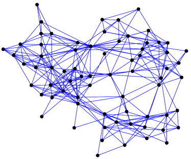
Figure 4: A layout of a highschool social network (MH), using the Fruchterman–Reingold algorithm (Fruchterman & Reingold, 1991).

6.2 Temporal Distribution

The temporal distributions shows the distribution of edge creation times. It is only defined for networks with known edge creation times. The X axis is the time, and the Y axis is the number of edges added during each time interval.

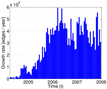
Figure 5: The temporal distribution of edges for the Wikipedia elections network.

6.3 Edge Weight and Multiplicity Distribution

The edge weight and multiplicity distribution plots show the distribution of edge weights and of edge multiplicities, respectively. They are not generated for unweighted networks. The X axis shows values of the edge weights or multiplicities, and the Y axis shows frequencies. Edge multiplicity distributions are plotted on doubly logarithmic scales.

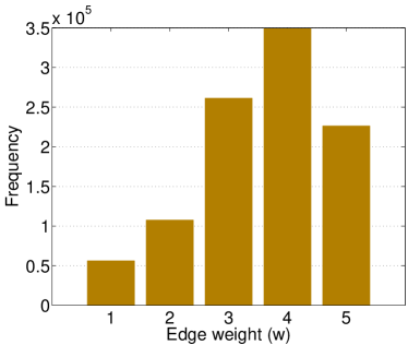
(a) Edge weight distribution

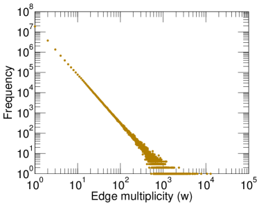
(b) Edge multiplicity distribution

Figure 6: The distribution of (a) edge weights for the MovieLens rating network (M2) and (b) edge multiplicities for the German Wikipedia edit network (de).

6.4 Degree Distribution

The distribution of degree values $d(u)$ over all vertices $u$ characterizes the network as a whole, and is often used to visualize a network. In particular, a power law is often assumed, stating that the number of nodes with $n$ neighbors is proportional to $n^{-\gamma}$, for a constant $\gamma$ (Barabási & Albert, 1999). This assumption can be inspected visually by plotting the degree distribution on a doubly logarithmic scale, on which a power law renders as a straight line. KONECT supports two different plots: The degree distribution, and the cumulative degree distribution. The degree distribution shows the number of nodes with degree $n$, in function of $n$. The cumulative degree distribution shows the probability that the degree of a node picked at random is larger than $n$, in function of $n$. Both plots use a doubly logarithmic scale.

Another visualization of the degree distribution supported by KONECT is in the form of the Lorenz curve, a type of plot to measure inequality originally used in economics (not shown).

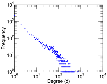
(a) Degree distribution

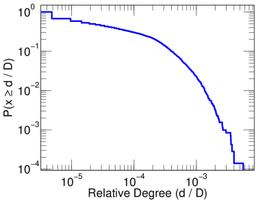
(b) Cumulative degree distribution

Figure 7: The degree distribution and cumulative degree distribution for the Wikipedia election network (EL).

The Lorenz curve is a tool originally from economics that visualizes statements of the form “X% of nodes with smallest degree account for Y% of edges”. The set of values $(X,Y)$ thus defined is the Lorenz curve. In a network the Lorenz curve is a straight diagonal line when all nodes have the same degree, and curved otherwise (Kunegis & Preusse, 2012). The area between the Lorenz curve and the diagonal is half the Gini coefficient (see above).

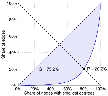
Figure 8: The Lorenz curve for the Wikipedia election network (EL).

6.5 Out/indegree Comparison

The out/indegree comparison plots show the joint distribution of outdegrees and indegrees of all nodes of directed graphs. The plot shows, for one directed network, each node as a point, which the outdegree on the X axis and the indegree on the Y axis.

An example is shown in Figure 9 for the Wikipedia elections network.

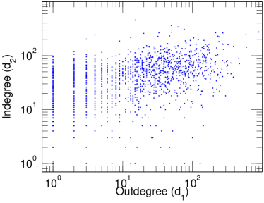
Figure 9: The out/indegree comparison plot of the Wikipedia election network (EL).

6.6 Assortativity Plot

In some networks, nodes with high degree are more often connected with other nodes of high degree, while nodes of low degree are more often connected with other nodes of low degree. This property is called assortativity, i.e., such networks are said to be assortativity. On the other hand, some networks, are dissortative, i.e., in them nodes of high degree are more often connected to nodes of low degree and vice versa. In addition to the assortativity $\rho$ defined as the Pearson correlation coefficient between the degrees of connected nodes, the assortativity or dissortativity of networks may be analyse by plotting all nodes of a network by their degree and the average degree of their neighbors. Thus, the assortativity plot of a network shows all nodes of a network with the degree on the X axis, and the average degree of their neighbors on the Y axis.

An example of the assortativity plot is shown for the Wikipedia elections network in Figure 10.

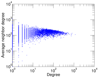
Figure 10: The assortativity plot of the Wikipedia election network (EL).

6.7 Clustering Coefficient Distribution

In Section 4.5, we defined the clustering coefficient of a node in a graph as the propotion of that node’s neighbors that are connected, and proceeded to define the clustering coefficient as the corresponding measure applied to the whole network. In some case however, we may be interested in the distribution of the clustering coefficient over the nodes in the network. For instance, a network could have some very clustered parts, and some less clustered parts, while another network could have many nodes with a similar, average clustering coefficient. Thus, we may want to consider the distribution of clustering coefficient. This distribution can be plotted as a cumulated plot.

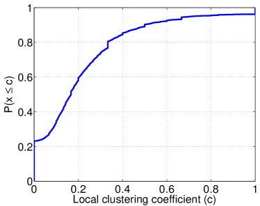
Figure 11: The clustering coefficient distribution for Facebook link network (Ol).

6.8 Spectral Plot

The eigenvalues of a network’s characteristic matrices $\mathbf{A}$, $\mathbf{N}$ and $\mathbf{L}$ are often used to characterize the network as a whole. KONECT supports computing and visualizing the spectrum (i.e., the set of eigenvalues) of a network in multiple ways. Two types of plots are supported: Those showing the top-$k$ eigenvalues computed exactly, and those showing the overall distribution of eigenvalues, computed approximately. The eigenvalues of $\mathbf{A}$ are positive and negative reals, the eigenvalues of $\mathbf{N}$ are in the range $[-1,+1]$, and the eigenvalues of $\mathbf{L}$ are all nonnegative. For $\mathbf{A}$ and $\mathbf{N}$, the largest absolute eigenvalues are used, while for $\mathbf{L}$ the smallest eigenvalues are used. The number of eigenvalue shown $k$ depends on the network, and is chosen by KONECT such as to result in reasonable runtimes for the decomposition algorithms.

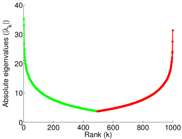
(a) Top-$k$ eigenvalues of $\mathbf{A}$

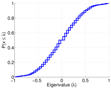
(b) Cumulative eigenvalue distribution of $\mathbf{N}$

Figure 12: The top-$k$ eigenvalues of $\mathbf{A}$ and the cumulative spectral distribution of $\mathbf{N}$ for the Wikipedia election network (EL). In the first plot (a), positive eigenvalues are shown in green and negative ones in red.

Two plots are generated: the non-cumulative eigenvalue distribution, and the cumulative eigenvalue distribution. For the non-cumulative distribution, the absolute $\lambda_{i}$ are shown in function of $i$ for $1\leq i\leq k$. The sign of eigenvalues (positive and negative) is shown by the color of the points (green and red). For the cumulated eigenvalue plots, the range of all eigenvalues is computed, divided into 49 bins (an odd number to avoid a bin limit at zero for the matrix $\mathbf{N}$), and then the number of eigenvalues in each bin is computed. The result is plotted as a cumulated distribution plot, with boxes indicating the uncertainty of the computation, due to the fact that eigenvalues are not computed exactly, but only in bins.

6.9 Complex Eigenvalues Plot

The adjacency matrix of an undirected graph is symmetric and therefore its eigenvalues are real. For directed graphs however, the adjacency matrix $\mathbf{A}$ is asymmetric, and in the general case its eigenvalues are complex. We thus plot, for directed graphs, the top-$k$ complex eigenvalues by absolute value of the adjacency matrix $\mathbf{A}$.

Three properties can be read off the complex eigenvalues: whether a graph is nearly acyclic, whether a graph is nearly symmetric, and whether a graph is nearly bipartite. If a directed graph is acyclic, its adjacency matrix is nilpotent and therefore all its eigenvalues are zero. The complex eigenvalue plot can therefore serve as a test for networks that are nearly acyclic: the smaller the absolute value of the complex eigenvalues of a directed graph, the nearer it is to being acyclic. When a directed network is symmetric, i.e., all directed edges come in pairs connecting two nodes in opposite direction, then the adjacency matrix $\mathbf{A}$ is symmetric and therefore all its eigenvalues are complex. Thus, a nearly symmetric directed network has complex eigenvalues that are near the real line. Finally, the eigenvalues of a bipartite graph are symmetric around the imaginary axis. In other words, if $a+bi$ is an eigenvalue, then so is $-a+bi$ when the graph is bipartite. Thus, the amount of symmetric along the imaginary axis is an indicator for bipartivity. Note that bipartivity here takes into account edge directions: There must be two groups such that all (or most) directed edges go from the first group to second. Figure 13 shows two examples of such plots.

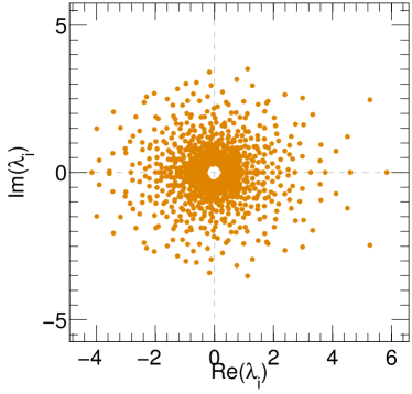
(a) Wikipedia elections

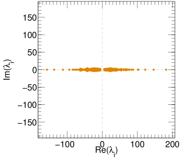
(b) UC Irvine messages

Figure 13: The top-$k$ complex eigenvalues $\lambda_{i}$ of the asymmetric adjacency matrix $\mathbf{A}$ of the directed Wikipedia election (EL) and UC Irvine messages (UC) networks.

6.10 Distance Distribution Plot

Distance statistics can be visualized in the distance distribution plot. The distance distribution plot shows, for each integer $k$, the number of node pairs at distance $k$ from each other, divided by the total number of node pairs. The distance distribution plot is also called the hop plot. The distance distribution plot can be used to read off the diameter, the median path length, and the 90-percentile effective diameter (see Section 4.6). For temporal networks, the distance distribution plot can be shown over time.

The non-temporal distance distribution plot shows the cumulated distance distribution function between all node pairs $(u,v)$ in the network, including pairs of the form $(u,u)$, whose distance is zero.

The temporal distance distribution plot shows the same data in function of time, with time on the X axis, and each colored curve representing one distance value.

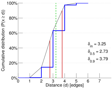
(a) Distance distribution plot

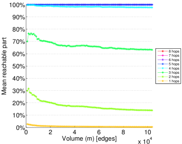
(b) Temporal distance distribution plot

Figure 14: The distance distribution plot and temporal distance distribution plot of the Wikipedia election network (EL).

6.11 Graph Drawings

A graph drawing is a representation of a graph, showing its vertices and egdes laid out in two (or three) dimensions in order for the graph structure to become visible. Graph drawings are easy to produce when a graph is small, and become harder to generate and less useful when a graph is larger.

Given a graph, a graph drawing can be specified by the placement of its vertices in the plane. To determine such a placement is a non-trivial problem, for which many algortihms exist, depending on the required properties of the drawing. For instance, each vertex should be placed near to its neighbors, vertices should not be drawn to near to each other, and edges should, if possible, not cross each other. It is clear that it is impossible to fulfill all these requirements at once, and thus no best graph drawing exists.

In KONECT, we show drawings of small graphs only, such that vertices and edges remain visible. The graph drawings in KONECT are spectral graph drawings, i.e., they are based on the eigenvectors of characteric graph matrices. In particular, KONECT included graph drawings based on the adjacency matrix $\mathbf{A}$, the normalized adjacency matrix $\mathbf{N}$ and the Laplacian matrix $\mathbf{L}$ (Koren, 2003). Let $\mathbf{x}$ and $\mathbf{y}$ be the two chosen eigenvector of each matrix, then the coordinate of the node $u\in V$ is given by $\mathbf{x}_{u}$ and $\mathbf{y}_{u}$.

For the adjacency matrix $\mathbf{A}$ and the normalized adjacency matrix $\mathbf{N}$, we use the two eigenvector with largest absolute eigevalue. For the Laplacian matrix $\mathbf{L}$, we use the two eigenvectors with smallest nonzero eigenvalue. Examples for the Zachary karate club social network (ZA) are shown in Figure 15.

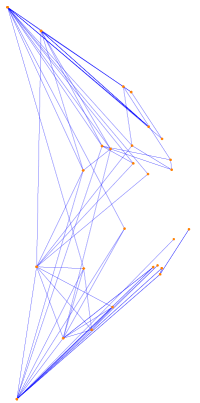
(a) Adjacency matrix $\mathbf{A}$

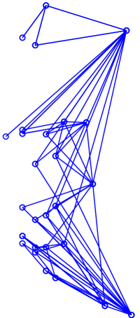
(b) Normalized adjacency matrix $\mathbf{N}$

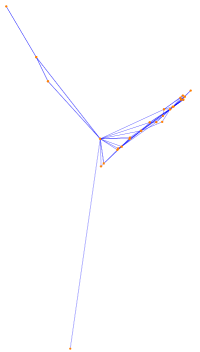
(c) Laplacian $\mathbf{L}$

Figure 15: Drawings of the Zachary karate club social network (ZA) using (a) the adjacency matrix $\mathbf{A}$, (b) the normalized adjacency matrix $\mathbf{N}$, (c) the Laplacian matrix $\mathbf{L}$.

7 Graph Decompositions

In order to analyse graphs, algebraic graph theory is a common approach. In algebraic graph theory, a graph with $n$ vertices is represented by an $n\times n$ matrix called the adjacency matrix, from which other matrices can be derived. The defined matrices can then be decomposed to reveal properties of the graph. In this section, we review characteristic graph matrices, their decompositions, and their uses. Since most decompositions are based on a specific matrix, this section also serves as a survey of characteristic graph matrices.

Graph decompositions are implemented in the KONECT Toolbox by the konect_decomposition() function. Each decomposition has a name, which is given in the margin in the following.

7.1 Decompositions of Undirected Graphs

These matrices and decompositions apply to undirected graphs.

In KONECT, these decompositions can be applied to directed graphs, in which case edge directions are ignored.

7.1.1 Symmetric Adjacency Matrix ($\mathbf{A}$)

The symmetric adjacency matrix $\mathbf{A}$ is the most basic graph characteristic matrix. It is a symmetric $n\times n$ matrix defined as $\mathbf{A}_{uv}=1$ when the nodes $u$ and $v$ are connected, and $\mathbf{A}_{uv}=0$ when $u$ and $v$ are not connected.

The eigenvalue decomposition of the matrix $\mathbf{A}$ for undirected graphs is widely used to analyse graphs:

$$\marginpar{\normalcolor\raggedright\texttt{sym}}\mathbf{A}\@add@raggedright =\mathbf{U}\mathbf{\Lambda}\mathbf{U}^{\mathrm{T}}$$ (97)

$\mathbf{\Lambda}$ is an $n\times n$ real diagonal matrix containing the eigenvalues of $\mathbf{A}$, i.e., $\mathbf{\Lambda}_{ii}=\lambda_{i}[\mathbf{A}]$. $\mathbf{U}$ is an $n\times n$ orthogonal matrix having the corresponding eigenvectors as columns.

The largest absolute eigenvalue of $\mathbf{A}$ is the networks spectral norm, i.e.,

$$\max_{i}|\mathbf{\Lambda}_{ii}| =\left\|\mathbf{A}\right\|_{2}.$$

The sum of all eigenvalues $\lambda_{i}$ equal the trace of $\mathbf{A}$, i.e., the sum of its diagonal elements. The sum of the eigenvalues of $\mathbf{A}$ thus equals the number of loops in the graphs. In particular, when a graph has no loops, then the sum of the eigenvalues of its adjacency matrix is zero.

Higher moments the eigenvalues of $\mathbf{A}$ give the number of tours in the graph. Remember that a tour of length $k$ is defined as a sequence of $k$ connected nodes, such that the first and the last node are connected, such that two tours are considered as distinct when they have a different starting node or orientation. The sum of $k$^th powers of the eigenvalues of $\mathbf{A}$ then equals the number of $k$-tours $T_{k}$. We thus have in a loopless graph, that the traces of powers of $\mathbf{A}$ are related to the number of edges $m$, the number of triangles $t$, the number of squares $q$ and the number of wedges $s$ by:

$$\mathrm{Tr}(\mathbf{A}) =0$$

$$\mathrm{Tr}(\mathbf{A}^{2}) =2m$$

$$\mathrm{Tr}(\mathbf{A}^{3}) =6t$$

$$\mathrm{Tr}(\mathbf{A}^{4}) =8q+4s+2m$$

The traces of $\mathbf{A}$ can also be expressed as sums of powers (moments) of the eigenvalues of $\mathbf{A}$:

$$\mathrm{Tr}(\mathbf{A}^{k}) =\sum_{i=1}^{n}\lambda_{i}^{k}$$

The spectrum of $\mathbf{A}$ can also be characterized in terms of graph bipartivity. When the graph is bipartite, then all eigenvalues come in pairs $\{\pm\lambda\}$, i.e., they are distributed around zero symmetrically. When the graph is not bipartite, then their distribution is not symmetric. It follows that when the graph is bipartite, the smallest and largest eigenvalues have the same absolute value.

7.1.2 Laplacian Matrix ($\mathbf{L}$)

The Laplacian matrix of an undirected graph is defined as

$$\mathbf{L} =\mathbf{D}-\mathbf{A},$$

i.e., the diagonal degree matrix from which we subtract the adjacency matrix.

We consider the eigenvalue decomposition of the Laplacian:

$$\marginpar{\normalcolor\raggedright\texttt{lap}}\mathbf{L}\@add@raggedright =\mathbf{U}\mathbf{\Lambda}\mathbf{U}^{\mathrm{T}}$$

The Laplacian matrix of positive-semidefinite, i.e., all eigenvalues are nonnegative. When the graph is unsigned, the smallest eigenvalue is zero and its multiplicity equals the number of connected components in the graph.

The second-smallest eigenvalue is called the algebraic connectivity of the graph, and is denoted $a=\lambda_{2}[\mathbf{L}]$ (Fiedler, 1973). If the graph is unconnected, that value is zero, i.e., an unconnected graph has an algebraic connectivity of zero.

When the graph is connected, the eigenvector corresponding to eigenvalue zero is a constant vector, i.e., a vector with all entries equal. The eigenvector corresponding the the second-smallest eigenvalue is called the Fiedler vector, and can be used to cluster nodes in the graph. Together with further eigenvectors, it can be used to draw graphs (Kunegis et al., 2010).

When the graph is signed, i.e., when the grpah admits edges with negative weights, then the smallest eigenvalue of $\mathbf{L}$ is called the algebraic conflict $\xi$. It is zero if and only if the graph is balanced, i.e., when the nodes can be divided into two groups such that all positive edges connect nodes within the same group, and all negative edges connect nodes of different groups. Equivalently, $\xi$ is larger than zero if and only if each connected component contains at least one cycle with an odd number of negative edges.

7.1.3 Normalized Adjacency Matrix ($\mathbf{N}$)

The normalized adjacency matrix $\mathbf{N}$ of an undirected graph is defined as

$$\mathbf{N} =\mathbf{D}^{-1/2}\mathbf{A}\mathbf{D}^{-1/2},$$

where we remind the reader that the diagonal matrix $\mathbf{D}$ contains the node degrees, i.e., $\mathbf{D}_{uu}=d(u)$. The matrix $\mathbf{N}$ is symmetric and its eigenvalue decomposition can be considered:

$$\marginpar{\normalcolor\raggedright\texttt{sym-n}}\mathbf{N}=\mathbf{U}\mathbf{\Lambda}\mathbf{U}^{\mathrm{T}}\@add@raggedright$$ (98)

The eigenvalues $\lambda_{i}$ of $\mathbf{N}$ can be used to characterize the graph, in analogy with those of the nonnormalized adjacency matrix. The spectrum of $\mathbf{N}$ is also called the weighted spectral distribution (Fay, 2010). All eigenvalues of $\mathbf{N}$ are contained in the range $[-1,+1]$. When the graph is unsigned, the largest eigenvalue is one. In addition, the eigenvalue one has multiplicity one if the graph is connected and unsigned. It follows that for general unsigned graphs, the multiplicity of the eigenvalue one equals the number of connected components of the graph.

Minus one is the smallest eigenvalue of $\mathbf{N}$ if and only iff the graph is bipartite. As with the nonnormalized adjacency matrix, the eigenvalues of $\mathbf{N}$ are distributed symmetrically around zero if and only if the graph is bipartite.

When the graph is connected, the eigenvector corresponding to eigenvalue one has entries proportional to the square root of node degrees, i.e.,

$$\mathbf{U}_{u1} =\sqrt{\frac{d(u)}{2m}}.$$

Note that this equivalence only holds for undirected graphs. For directed graphs, there is no such equivalence.

7.1.4 Normalized Laplacian Matrix ($\mathbf{Z}$)

The Laplacian matrix too, can be normalized. It turns out that the normalized Laplacian and the normalized adjacency matrix are tighly related to each other: They share the same set of eigenvectors, and their eigenvalues are reflections of each other.

The normalized Laplacian matrix of an undirected graph is defined as

$$\mathbf{Z} =\mathbf{D}^{-1/2}\mathbf{L}\mathbf{D}^{-1/2}.$$

As opposed to $\mathbf{A}$, $\mathbf{L}$ and $\mathbf{N}$, there is no standardized notation of the normalized Laplacian. The notation $\mathbf{Z}$ is specific to KONECT, and was chosen as the letter Z resembles a turned letter N, and the matrices represented by those letters share eigenvectors and have flipped eigenvalues.

The normalized Laplacian is related to the normalized adjacency matrix by

$$\mathbf{Z} =\mathbf{I}-\mathbf{N}=\mathbf{I}-\mathbf{D}^{-1/2}\mathbf{A}\mathbf{D}^{-1/2},$$

as can be derived directly from their definitions. It follows that $\mathbf{Z}$ and $\mathbf{N}$ have the same set of eigenvectors, and that their eigenvalues are related by the transformation $1-\lambda$. Thus, the properties of $\mathbf{Z}$ can be derived from those of $\mathbf{N}$. For instance, all eigenvalues of $\mathbf{Z}$ are contained in the range $[0,2]$, and the multiplicity of the eigenvalue zero equals the number of connected components (when the graph is unsigned). If the undirected graph is connected, the eigenvector of eigenvalue zero contains entries proportional to the square root of the node degrees.

In KONECT, the decomposition of the normalized Laplacian is not included, since it can be derived from that of the normalized adjacency matrix.

7.1.5 Stochastic Adjacency Matrix ($\mathbf{P}$)

The matrix

$$\marginpar{\normalcolor\raggedright\texttt{stoch1}}\mathbf{P}\@add@raggedright =\mathbf{D}^{-1}\mathbf{A}$$

is called the stochastic adjacency matrix. This matrix is asymmetric, even when the graph is undirected, except when the graph is regular, i.e., when all degrees are the same. Thus, its eigenvalue decomposition is not always defined, and in any case may not involve orthogonal matrices.

For directed graphs we may distinguish the right-stochastic (or row-stochastic) matrix $\mathbf{D}^{-1}\mathbf{A}$ and the left-stochastic (or column-stochastic) matrix $\mathbf{A}\mathbf{D}^{-1}$. Note the subtle terminology: $\mathbf{D}^{-1}\mathbf{A}$ is left-normalized but right-stochastic.

This matrix is related to the normalized adjacency matrix $\mathbf{N}$ by

$$\mathbf{P} =\mathbf{D}^{-1/2}\mathbf{N}\mathbf{D}^{1/2}$$

and therefore both matrices have the same set of eigenvalues. Thus, the eigenvalues of $\mathbf{P}$ are all real, even though $\mathbf{P}$ is asymmetric, and they are contained in the range $[-1,+1]$. Also, the relationship between $\mathbf{P}$ and $\mathbf{N}$ implies that that eigenvectors of $\mathbf{P}$ are related to those of $\mathbf{N}$ by factors of the diagonal elements of $\mathbf{D}^{1/2}$, i.e., the square roots of node degrees. Since $\mathbf{P}$ is asymmetric, its left eigenvectors differ from its right eigenvectors. When the graph is undirected, the left eigenvector corresponding to the eigenvalue one has entries proportional to the degree of nodes, while the right eigenvector corresponding to the eigenvalue one is the constant vector. This is consistent with the fact that for a random walk on an undirected graph, the stationary distribution of nodes is proportional to the node degrees.

The alternative matrix $\mathbf{A}\mathbf{D}^{-1}$ can also be considered. It is left-stochastic, and can be derived by considering random walks that tranverse edges in a backward direction.

The matrix $\mathbf{P}$ is the state transition matrix of a random walk on the graph, and thus its largest eigenvector is one if the graph is (strongly) connected. The matrix $\mathbf{P}$ is also related to the PageRank matrix $\mathbf{G}$ (“Google matrix”), which equals

$$\mathbf{G} =(1-\alpha)\mathbf{P}+\alpha\mathbf{J}$$

where $0<\alpha<1$ is a damping factor (the teleportation probability), and $\mathbf{J}$ is the matrix containing all ones. The left eigenvalues of the PageRank matrix give the PageRank values, and thus we see that (ignoring the teleportation term), the PageRank of nodes in an undirected network equals the degrees of the nodes.

The matrix $\mathbf{P}$ is also related to random walks with restarts on the graph, i.e., random walks that have a certain probability $0<\alpha<1$ to return to an initial node at each step, instead of taking an edge at random. For any two nodes $u$ and $v$, the number

$$\left[\alpha(\mathbf{I}-(1-\alpha)\mathbf{P}^{\mathrm{T}})^{-1}\right]_{uv}$$ (99)

gives the asymptotic probability that a random walk with restart starting at node $u$ stays at node $v$.

7.1.6 Stochastic Laplacian Matrix ($\mathbf{S}$)

A further variant of the Laplacian exists, based on the stochastic adjacency matrix:

$$\mathbf{S} =\mathbf{I}-\mathbf{P}=\mathbf{I}-\mathbf{D}^{-1}\mathbf{A}=\mathbf{I}-\mathbf{D}^{-1/2}\mathbf{N}\mathbf{D}^{1/2}=\mathbf{D}^{-1/2}\mathbf{Z}\mathbf{D}^{1/2}$$

This matrix shares much properties with $\mathbf{P}$ and thus with $\mathbf{N}$ and $\mathbf{Z}$. The eigenvalues of $\mathbf{S}$ are contained in the interval $[0,2]$. The eigenvalue zero has a multiplicity equal to the number of connected components of the graph, and when the graph is connected its corresponding right eigenvector is the constant vector, while its corresponding left eigenvector is proportional to the node degrees. For connected graphs, the largest eigenvalue of $\mathbf{S}$ is two if and only if the graph is bipartite. In the general case, the eigenvalue two has a multiplicity equal to the number of connected components that are bipartite.

7.1.7 Signless Laplacian ($\mathbf{K}$)

The signless Laplacian of a graph is defined as the Laplacian of the corresponding graph in which all edges are interpreted as negative. It thus equals

$$\marginpar{\normalcolor\raggedright\texttt{lapq}}\mathbf{K}\@add@raggedright =\mathbf{D}+\mathbf{A}$$ (100)

This matrix is positive-semidefinite, and its smallest eigenvalue is zero if and only if the graph is bipartite. Thus, $\mathbf{K}$ is used in measures of bipartivity.

7.1.8 Alternative Signed Laplacian

The Laplacian matrix $\mathbf{L}=\mathbf{D}-\mathbf{A}$ as defined earlier is based on the the degree matrix $\mathbf{D}$, whose diagonal elements equal the sum of absolute weights of all edges incident to each node. Taking the absolute value in that definition is justified for many applications related to signed graphs, and results in a positive-semidefinite matrix, whose smallest eigenvalue is zero if and only if there is at least one balanced component in the signed network. Alternatively, using the sum of edge weights instead results in a different matrix, which may have negative eigenvalues. This matrix appears in certain contexts; see e.g. the examples given by Bronski & DeVille (2014).

7.2 Decompositions of Directed Graphs

In directed graphs, the adjacency matrix $\mathbf{A}$ is itself asymmetric, and there is no special half-adjacency matrix. Since the adjacency matrix is symmetric, decompositions are more complex. For instance, $\mathbf{A}$ is not normal in the general case, and therefore there is no simply defined eigenvalue decomposition anymore.

7.2.1 Singular Value Decomposition

The singular value decomposition is defined for any matrix, including those that are not symmetric, and even those that are not quadratic. Thus, it can be applied to the adjacency matrix of directed graphs.

$$\marginpar{\normalcolor\raggedright\texttt{svd}}\mathbf{A}\@add@raggedright =\mathbf{U}\mathbf{\Sigma}\mathbf{V}^{\mathrm{T}}$$ (101)

The matrices $\mathbf{U}$ and $\mathbf{V}$ are each orthogonal, but they are not equal. They contain the left and right singular vectors are columns. The matrix $\mathbf{\Sigma}$ is diagonal, and contains the singular values, which are all nonnegative.

7.2.2 Normalized Adjacency Matrix

The adjacency matrix can be normalized for directed network, in the same way as for undirected networks.

$$\mathbf{N} =\mathbf{D}_{\mathrm{O}}^{-1/2}\mathbf{A}\mathbf{D}_{\mathrm{I}}^{-1/2}$$ (102)

Here, $\mathbf{D}_{\mathrm{O}}^{-1/2}$ and $\mathbf{D}_{\mathbf{I}}^{-1/2}$ are the diagonal matrices of out- and indegrees.

The normalized adjacency matrix $\mathbf{N}$ can be used in the singular value decomposition, too:

$$\marginpar{\normalcolor\raggedright\texttt{svd-n}}\mathbf{N}\@add@raggedright =\mathbf{U}\mathbf{\Sigma}\mathbf{V}^{\mathrm{T}}$$ (103)

7.2.3 Eigenvectors

While the eigenvalue decomposition is not defined in the general case for an asymmetric matrix $\mathbf{A}$, its eigenvectors and eigenvalues are well-defined, if we distinguish between left and right eigenvectors.

Thus, we define the method diag, which is a decomposition in the KONECT sense, but not in the strict mathematical sense. $\mathbf{U}$ and $\mathbf{V}$ are then defined as the matrices containing the left and right eigenvectors of $\mathbf{A}$, and $\mathbf{\Lambda}$ is the diagonal matrix of corresponding eigenvalues.

Note that while left and right eigenvectors differ, their eigenvalues are identical.

7.2.4 Skew Adjacency Matrix ($\mathbf{Y}$)

While an asymmetric matrix $\mathbf{A}$ may be transformed to $\mathbf{A}+\mathbf{A}^{\mathrm{T}}$ to give a symmetric matrix, we can also use $\mathbf{Y}=\mathbf{A}-\mathbf{A}^{\mathrm{T}}$ to get a skew-symmetric matrix. A skew symmetric matrix $\mathbf{X}$ is a matrix such that $\mathbf{X}=-\mathbf{X}^{\mathrm{T}}$.

Skew symmetric matrices have well-defined eigenvalue decompositions, which are however complex, as both the eigenvectors and eigenvalues will be complex numbers. The eigenvectors and eigenvalues however follow a specific pattern, that we can exploit to represent such a decomposition using only real numbers:

$$\mathbf{Y} =\mathbf{A}-\mathbf{A}^{\mathrm{T}}=\mathbf{Q}\mathbf{R}\mathbf{Q}^{\mathrm{T}}$$ (104)

such that

$$\mathbf{Q} =\frac{1}{\sqrt{2}}\left[\begin{array}[]{cc}\mathbf{U}+i\mathbf{V}\\ \mathbf{U}-i\mathbf{V}\end{array}\right]$$ (107)

$$\mathbf{R} =\left[\begin{array}[]{cc}i\mathbf{D}&\mathbf{0}\\ \mathbf{0}&-i\mathbf{D}\end{array}\right]$$ (110)

where $\mathbf{U}$, $\mathbf{V}$ and $\mathbf{D}$ are real matrices. In fact, this decomposition can be equivalently written as

$$\marginpar{\normalcolor\raggedright\texttt{skew}}\mathbf{Y}=\mathbf{A}-\mathbf{A}^{\mathrm{T}}\@add@raggedright =\mathbf{U}\mathbf{D}\mathbf{V}^{\mathrm{T}}-\mathbf{V}\mathbf{D}\mathbf{U}^{\mathrm{T}}.$$ (111)

This decomposition is equivalent to that given by Constantine & Gower (1978). It shows that the skew-symmetric matrix $\mathbf{Y}$ has eigenvalues that are purely imaginary, come in pairs $\{\pm i\lambda\}$ that are the negative of each other (or equivalently, the complex conjugate), and their corresponding eigenvectors are also complex conjugates of each other.

Note also that the number of columns of both $\mathbf{U}$ and $\mathbf{V}$ is at most $\lfloor n\rfloor$, and thus, if $n$ is odd, the skew-symmetric matrix $\mathbf{Y}$ has the eigenvalue zero, which is the complex conjugate of itself. Also, the expression $\mathbf{U}\mathbf{D}\mathbf{V}^{\mathrm{T}}$ is not the singular value decomposition of $\mathbf{A}$, even if the form of the decomposition is the same.

7.2.5 Hermitian Adjacency Matrix ($\mathbf{H}$)

In certain contexts, for instance when constructing the Hamiltonian of a system, it is necessary to specify Hermitian matrices, i.e., diagonalizable matrices that have only real eigenvalues. To take into account all connectivity information of a directed graph in a directed graph, the symmetric and skew-symmetric adjacency matrices can be combined in the following way:

$$\marginpar{\normalcolor\raggedright\texttt{herm}}\mathbf{H}\@add@raggedright =\frac{1}{\sqrt{2}}\left[\mathbf{A}+\mathbf{A}^{\mathrm{T}}+i(\mathbf{A}-\mathbf{A}^{\mathrm{T}})\right].$$ (112)

The matrix $\mathbf{H}$ is Hermitian, i.e., it equals the complex conjugate of its transpose, $\mathbf{H}=\mathbf{\bar{H}}^{\mathrm{T}}=\mathbf{H}^{\dagger}$. Furthermore, the Hermitian adjacency matrix can be defined by

$$\mathbf{H}_{uv} =\exp\left\{i\frac{\pi}{4}\mathbf{Y}_{uv}\right\},$$ (113)

which additionally justifies the factor $1/\sqrt{2}$ in the initial definition of $\mathbf{H}$, as $e^{i\frac{\pi}{4}}=1/\sqrt{2}+i/\sqrt{2}$. Using this form, the Hermitian adjacency matrix can be generalized to the matrix $\mathbf{H}_{\alpha}$ where $0\leq\alpha\leq\pi/2$ is a real parameter, giving

$$[\mathbf{H}_{\alpha}]_{uv} =\exp\left\{i\alpha\mathbf{Y}_{uv}\right\},$$ (114)

from which the following special cases can be recovered:

$$\mathbf{H}_{0} =\mathbf{A}+\mathbf{A}^{\mathrm{T}},$$ (115)

$$\mathbf{H}_{\pi/4} =\mathbf{H},$$ (116)

$$\mathbf{H}_{\pi/2} =\mathbf{Y}.$$ (117)

These matrices appear in the modeling of quantum walks, as used for instance by Tödtli et al. (2016).

8 The KONECT Toolbox

The KONECT Toolbox for Matlab is a set of functions for the Matlab programming language containing implementations of statistics, plots and other network analysis methods. The KONECT Toolbox is used to generate the numerical statistics and plots in this handbook as well as on the KONECT website.

Installation

The KONECT Toolbox is provided as a directory containing *.m files. The directory can be added to the Matlab path using addpath() to be used.

Usage

All functions have names beginning with konect_.

8.1 Examples

This section gives short example for using the toolbox. The examples can be executed in Matlab.

Load a unipartite dataset

This example loads the Slashdot signed social network.

T = load(’out.slashdot-zoo’);
n = max(max(T(:,1:2)));
A = sparse(T(:,1), T(:,2), T(:,3), n, n);

This loads the weighted adjacency matrix of the Slashdot Zoo into the matrix A.

8.2 Variables

Naming variables can be quite complicated and hard to read in Matlab. Therefore KONECT code follows these rules.

Long variable names (containing full words) are in all-lowercase. Words are separated by underscore. When refering to a variable in comments, the variable is written in all-uppercase. Short variable names (letters) are lowercase for numbers and vectors, and uppercase for matrices.

8.2.1 Strings

Table 5 shows common variable names used for string variables.

Table 5: Long variable names of string type used in KONECT.

network	The internal network name, e.g., “advogato”. The internal network name is used in the names of files related to the network.
class	The internal name for a set of networks, e.g., “test”, “1”, “2”, “3”. The class “N” includes the $10\times N$ smallest networks.
code	The 1/2/3-character code for a network, e.g., “EN” for Enron.
curve	The internal name of a curve fitting method.
decomposition	The internal of a matrix decomposition, as passed to the function konect_decomposition(), e.g., “sym”, “asym” and “lap”.
feature	The internal name of a feature, e.g., “degree” and “decomp.sym”.
filename	A filename.
format	The network format in lower case as defined in the function konect_consts(), e.g., “sym” and “bip”.
label	The readable name of things used in plots, tables, etc.
measure	The internal name of a measure of link prediction accuracy, e.g., “map” and “auc”.
method	The internal name of a link prediction method.
statistic	The internal name of a network statistic, e.g., “power” and “alcon”.
transform	The name of a transform, e.g. “simple” and “lcc”.
type	The internal name of the computation type. This can be “split” or “full”. This decides which version of a network gets used, in particular for time-dependent analyses.
weights	The edge weight type as defined in the function konect_consts(), e.g., “unweighted” and “signed”.

8.2.2 Scalars

Table 6 shows variable names used for scalar values.

Table 6: Variable names used for scalars in KONECT.

n, n1, n2	Row/column count in matrices, left/right vertex count
r	Rank of a decomposition
m	Edge count
i, j	Vertices as integer, i.e., indexes in rows and columns.
prediction	A link prediction score, i.e., a value returned by a link prediction algorithm for a given node pair.
precision	The prediction accuracy value, typically between 0 and 1.
means	Values used for additive (de)normalization, as a structure.

8.2.3 Matrices

Table 7 shows variable names used for matrix-valued variables.

Note that when the adjacency matrix of an undirected graph is stored in a variable, each edge is usually stored just once, instead of twice. In other words, the variable A for undirected networks does not equal the matrix $\mathbf{A}$, instead the expression A + A’ does.

Table 7: Variable names used for matrices and vectors in KONECT. As a general rule, matrices have upper-case names and vectors have lower-case names.

A	($n\times n$) Adjacency matrix (in code where the adjacency and biadjacency matrix are distinguished)
A	($n\times n$ or $n_{1}\times n_{2}$) Adjacency or biadjacency matrix (in code where the two are not distinguished)
B	($n_{1}\times n_{2}$) Biadjacency matrix (in code where the adjacency and biadjacency matrix are distinguished)
D	($r\times r$) Central matrix; e.g., eigenvalues; as matrix
dd	($r\times 1$) Diagonal of the central matrix
E	($e\times 2$) Test set for link prediction, stored in the same way as T
L	($n\times n$) Laplacian matrix
M, N	Normalized (bi)adjacency matrix
T	($m\times 2$ or $m\times 3$ or $m\times 4$) Compact adjacency matrix, as stored in out.* files, and such that it can be converted to a sparse matrix using konect_spconvert().
	First column: row IDs
	Second column: column IDs
	Third column (optional): edge weights (1 if not present)
	Fourth column (optional): timestamps in Unix time
U	($n\times r$ or $n_{1}\times r$) Left part of decomposition; e.g., left eigenvectors
V	($n\times r$ or $n_{2}\times r$) Right part of decomposition; e.g., right eigenvectors
X	($r\times r$) Central matrix, when explicitly nondiagonal
Z	($n\times n$) Normalized Laplacian matrix

8.2.4 Compound Types

A struct containing elements whose names are of a specific type are named [VALUETYPE]s_[KEYTYPE]. For instance, a struct with labels used for methods is named as follows:

labels_method.(’auc’) = ’Area under the curve’;

Note:

• The first element is the name of the content type.

• The plural is used only for the content type.

8.2.5 IDs

Variables named method, decomposition, etc. are always strings. If a method, decomposition or any other type is represented as an integer (e.g., as an index into an array), then _id is appended to the variable name. For instance:

decomposition = ’sym’; decomposition_id = 2;

This means that an array of values by ID of keys is called for instance:

labels_decomposition_id{1} = ’Eigenvalue decomposition’;
labels_decomposition_id{2} = ’Singular value decomposition’;

9 File Formats

Due to the ubiquity of networks in many areas, there are a large number of file formats for storing graphs and graph-like structures. Some of these are well-suited for accessibility from many different programming languages (mostly line-oriented text formats), some are well-suited for integration with other formats (semantic formats such as RDF and XML-based ones), while other formats are optimized for efficient access (binary formats). In KONECT, we thus use three file formats covering the three cases:

• Text format: This format is text-based and uses tab-separated values. This is the main KONECT data format from which the two others are derived. The format has the advantage that it can be read easily from many different programming languages and environment.

• RDF format: Datasets are also available as RDF. This is intended for easy integration with other datasets.

• Matlab format: To compute statistics and plots and perform experiments, we use Matlab’s own binary format, which can be accessed efficiently from within Matlab.

In the following, we describe KONECT’s text format. Each network $NETWORK is represented by the following files:

• out.$NETWORK: The edges stored as tab separated values (TSV). The file is a text file, and each line contains information about one edge. Each line contains two, three or four numbers represented textually, and separated by any sequence of whitespace. The preferred separator is a single tab. The first two columns are mandatory and contain the source and destination node ID of the edge. The third column is optional and contains the edge weight. When the network is dynamic, the third column contains $+1$ for added edges and $-1$ for removed edges. For unweighted, non-temporal networks, multiple edges may be aggregated into a single line containing, in the third column, the number of aggregated edges. The fourth column is optional and contains the edge creation time, and is stored as UNIX time, i.e., the number of seconds since 1 January 1970. The fourth column is usually an integer, but may contain floating point numbers. If the fourth column is present, the third column must also be given. The beginning of the file contains additional comment lines with the following information:

        % FORMAT WEIGHTS
        % RELATIONSHIP-COUNT SUBJECT-COUNT OBJECT-COUNT
      
  

  where FORMAT is the internal name for the format as given in Table 1, WEIGHTS is the internal name for the weight types as given in Table 2, RELATIONSHIP-COUNT is the number of data lines in the file, and SUBJECT-COUNT and OBJECT-COUNT both equal the number of nodes $n$ in unipartite networks, and the number of left and right nodes $n_{1}$ and $n_{2}$ in bipartite networks. The first line is mandatory; the second line is optional.

• meta.$NETWORK: This file contains metadata about the network that is independent of the mathematical structure of the network. The file is a text file coded in UTF-8. Each line contains one key/value pair, written as the key, a colon and the value. The following metadata are used:

  • name: The name of the dataset (usually only the name of the source, without description the type or category, e.g., “YouTube”, “Wikipedia elections”). The name uses sentence case. For networks with the same name the source (e.g., the conference) is added in parentheses. Within each category, all names must be distinct.

  • code: The short code used in plots and narrow tables. The code consists of two or three characters. The first two characters are usually uppercase letters and denote the data source. The last character, if present, usually distinguishes the different networks from one source.

  • url: (optional) The URL(s) of the data sources, as a comma separated list. Most datasets have a single URL.

  • category: The name of the category, as given in the column “Category” in Table 3.

  • description: (deprecated) A short description of the form “User–movie ratings”. Note that the file should contain an actual en dash, coded in UTF-8.

  • cite: (optional) The bibtex code(s) for this dataset, as a comma separated list. Most dataset have a single bibtex entry.

  • fullname: (optional) A longer name to disambiguate different datasets from the same source, e.g., “Youtube ratings” and “Youtube friendships”. Uses sentence case. All networks must have different fullnames.

  • long-description: (optional, recommended) A long descriptive text consisting of full sentences, and describing the dataset in a verbose way. HTML markup may be used sparingly (tags: I, etc.), usually only for absolutely necessary typography, such as setting species names in italics.

  • entity-names: A comma-seperated list of entity names (e.g., “user, movie”). Unipartite networks give a single name; bipartite networks give two.

  • relationship-names: The name of the relationship represented by edges, as a substantive (e.g., “friendship”).

  • extr: (optional) The name of the subdirectory that contains the extraction code for this dataset.

  • timeiso: (optional) A single ISO timestamp denoting the date of the dataset or two timestamps separated by a slash(/) for a time range. The format is: YYYY[-MM[-DD]][/YYYY[-MM[-DD]]], e.g., “2005-10-08/2006-11-03” or “2007”.

  • tags: (optional) A space-separated list of hashtags describing the network. The following tags are used:

    • #acyclic: The network is acyclic. Can only be set for directed networks. If this is not set, a directed network must contain at least two pairs of reciprocal edges of the form $(u,v)$ and $(v,u)$. If the network does not contain reciprocal edges, but has cycles, the tag #nonreciprocal is used.

    • #aggregatetime: The small value of timestamps stand for any earlier time; these timestamps should not be considered when performing time-based methods and plots.

    • #incomplete: The network is incomplete, i.e., not all edges or nodes are included. This implies that for instance its degree distribution is not meaningful.

    • #join: The network is actually the join of more fundamental networks. For instance, a co-authorship network is a join of the authorship network with itself. Networks that have this tag may have skewed properties, such as skewed degree distributions.

    • #kcore: The network contains only nodes with a certain minimal degree $k$. In other words, the nodes with degree less than a certain number $k$ were removed from the dataset. This changes a network drastically, and is called the “$k$-core” of a network. This is sometimes done to get a less sparse network in applications that do not perform well on sparse networks. This tag implies the #incomplete tag.

    • #lowmultiplicity: Set in networks with multiple edges in which the actual maximal edge multiplicity is very low. Used to be able to use the maximal multiplicity as a sanity check. Indicates a dataset error.

    • #missingorientation: This tag is used for undirected networks which are based on an underlying directed network. For instance, in a citation network, we may only know that the documents A and B are linked, but not which one cites the other. In such a case, the network in KONECT is undirected, although the underlying network is actually directed.

    • #lcc: The dataset actually contains only the largest connected component of the actual network. Implies #incomplete. This tag is not used when the network is connected for other reasons.

    • #loop: The network may contain loops, i.e., egdes connecting a vertex to itself. This tag is only allowed for unipartite networks. When this tag is not present, loops are not allowed, and the presence of loops will be considered an error by analysis code.

    • #nonreciprocal: For directed networks only. The network does not contain reciprocal edges.

    • #regenerate: The network can be regenerated periodically and may be updated when a more recent dataset becomes available.

    • #tournament: The graph is directed and for each pair of nodes $\{u,v\}$, either the directed edge $u\rightarrow v$ or the directed edge $v\rightarrow u$ exists, but not both. It is an error for a non-directed graph to have this tag. If #tournament is defined, then #nonreciprocal must also be defined. Also, #loop must not be defined.

    • #zeroweight: Must be set if it is allowed for edge weights to be zero. Only used for networks with positive edge weights and signed/multisigned networks.

  • n3-*: (optional) Metadata which is used for the generation of RDF files. The symbol {n} in the name of the meta key represents an order by unique, sequential numbers starting at 1.

    • n3-add-prefix{n} (optional): Used to define additional N3 prefixes. The default prefixes are specified in this way.

    • n3-comment-{n} (optional): Add commentary lines which are placed at the beginning of the N3 file.

    • n3-edgedata-{n} (optional): Additional N3-data, to be displayed with each edge.

    • n3-nodedata-m-{n} (optional): Additional N3-data, to be displayed with the first occurence of the source ID.

    • n3-nodedata-n-{n} (optional): Additional N3-data, to be displayed with the first occurence of the target ID.

    • n3-prefix-m: N3-prefix for the source IDs.

    • n3-prefix-n (optional): N3-prefix for the target IDs. If this field is left out, the value of {n3-prefix-m} is used.

    • n3-prefix-j (optional): Additional prefix which can be used with the source id, if there is an entity to be represented with the same id.

    • n3-prefix-k (optional): Additional prefix which can be used with the target id, if there is an entity to be represented with the same id. This is used for example in meta.facebook-wosn-wall for the representation of users walls.

    • n3-prefix-l (optional): N3-prefix for the edges, if they are to be represented by some N3-entity.

    • n3-type-l (optional): RDF-type for the edges.

    • n3-type-m: RDF-type for source IDs.

    • n3-type-n (optional): RDF-type for target IDs.

    The following symbols are used in the n3-expressions for edgedata and nodedata:

    • : n3-prefix-m + source ID

    • : n3-prefix-n (or n3-prefix-m if the other is undefined) + target ID

    • : source ID

    • : target ID

    • : edge ID

    • : edge timestamp

Appendix A Glossary of Terms

Some terms related to graph theory are well established in mathematics, network theory and computer science, while other terms do not have a widely-used definition. The choices made in this work are those of the authors, and were chosen to reflect best practices and to avoid confusion.

Adjacency matrix

The matrix describing a network, usually denoted $\mathbf{A}$. To be contrasted with the half-adjacency matrix (for undirected unipartite networks, also denoted $\mathbf{A}$) and the biadjacency matrix (for bipartite networks, denoted $\mathbf{B}$). The adjacency matrix is always square, and for undirected networks it is symmetric.

Arc

A directed edge. In general, we consider arcs to be a special cases of edges, and thus we rarely use the term arc in favor of directed edge. (In other texts, an edge is taken to be undirected by definition, and the term directed edge is then a contradiction.)

Biadjacency matrix

The characteristic matrix of a bipartite network, usually denoted $\mathbf{B}$. The corresponding adjacency matrix is then $[\mathbf{0},\mathbf{B};\mathbf{B}^{\mathrm{T}},\mathbf{0}]$.

Category

Networks have a category, which describes the domain they apply to: social networks, transport networks, citation networks, etc.

Central matrix

The matrix $\mathbf{X}$ in any decomposition of the form $\mathbf{U}\mathbf{X}\mathbf{V}^{\mathrm{T}}$, not necessarily diagonal or symmetric; a generalization of the diagonal eigenvalue matrix.

Class

The networks of KONECT are divided into classes by their volume: Class 1 contains the ten smallest networks, Class 2 contains the next ten smallest networks, etc.

Claw

Three edges sharing a single vertex. A claw can be understood as a 3-star.

Code

The two- or three-character code representation of a network. These are used in scatter plots that show many networks.

Cross

A pattern of four edges sharing a single endpoint. Also called a 4-star.

Curve

A curve fitting method used for link prediction, when using the link prediction method described in (Kunegis & Lommatzsch 2009) (learning spectral transformations).

Cycle

A cyclic sequence of connected edges, not containing any edge twice. A cycle contrasts with a tour, in which a single vertex can appear multiple times.

Decomposition

In KONECT the word decomposition is used to denote the combination of a characteristic graph matrix (e.g. the adjacency matrix or Laplacian) with a matrix decomposition. As an extension, some other constructions are also called decomposition, such as LDA.

Density

This word is avoided in KONECT. In the literature, it may refer to either the fill (probability that an edge exists), or to the average degree. The former definition is typically used in mathematical contexts, while the latter is used in computer science contexts.

Edge

A connection between two nodes. In mathematics, an edge is undirected and constrasts with an arc which is directed. In the context of KONECT, all types of connections between nodes are called edges and an arc is a special case of an edge.

Feature

A node feature. I.e., a number assigned to each node. Examples are the degree, PageRank and the eccentricity. Equivalently, a node vector.

Fill

The probability that two randomly chosen nodes are connected. Also called the density, in particular in a mathematical context. The fill is the sole parameter of the Erdős–Rényi random graph model. The word fill is specific to KONECT.

Format

The format of a network determines its general structure, and whether edges are directed. There are three possible formats: unipartite and undirected; unipartite and directed; and bipartite. Directed bipartite networks are not possible in KONECT. Possible future extensions would include hypergraphs (e.g., tripartite networks).

Half-adjacency matrix

The adjacency matrix $\mathbf{A}$ of an undirected graph contains two nonzero entries for each edge $\{i,j\}$: $\mathbf{A}_{ij}$ and $\mathbf{A}_{ji}$. To avoid this, KONECT code uses the half-adjacency matrix, which contains only one of the two nonzero entries. The half-adjacency matrix is therefore not unique, i.e., it is unspecified whether $\mathbf{A}_{ij}$ or $\mathbf{A}_{ji}$ is nonzero. In code, the half-adjacency matrix is denoted A. The term half-adjacency matrix is specific to KONECT, but the use of such a representation is widespread.

Measure

A measure of the accuracy of link prediction methods, for instance the area under the curve or the mean average precision.

Method

A link prediction method.

PageRank

A node-based feature of a directed network, defined as the dominant eigenvector of the matrix $\mathbf{G}=(1-\alpha)\mathbf{P}+\alpha\mathbf{J}$, with eigenvalue one.

Path

A sequence of connected nodes, in which each node can appear only once. The extension that allows multiple nodes is called a walk. A path with identical start and end nodes is called a cycle.

Score

A numerical value given to a node pair. Usually used for link prediction, but can also measure distance or similary between nodes.

Size

The number of nodes in a network.

Statistic

A statistic is a numerical measure of a network, i.e., a number that describes a network, such as the clustering coefficient, the diameter or the algebraic connectivity. All statistics are real numbers.

Tour

A cyclic sequence of connected nodes which may contain a single vertex multiple times. It can be considered a walk that returns to it starting point, or a generalization of a cycle that allows to visit nodes multiple times.

Transform

A transform is an operation that applies to a graph and that gives another graph. Examples are taking the largest connected component, removing multiple edges, and making a bipartite graph unipartite. Certain graph properties can be expressed as other graph properties applied to graph transforms. For instance, the size of the largest connected component is the size of the transform which keeps only the largest connected component.

Triangle

Three nodes all connected with each other. The number of triangles in a network is a commonly used statistic, used for instance as the basis to compute the clustering coefficient. Counting the triangles in a network is a very common computational problem.

Volume

The number of edges in a network.

Walk

A sequence of connected nodes, which may contain a single node multiple times. The restriction to include a single node only once is called a path. If the endpoints of a walk are identical, then the walk is also a tour.

Wedge

Two edges sharing a common node, i.e., two incident edges. The number of wedges in a network is an important network statistic, which characterizes that skewness of the degree distribution, and which can be easily calculated. A wedge can be seen as a 2-star or a 2-path.

Weights

(always in the plural) The weights of a network describe the range of edge weights it allows. The list of possible edge weights is given in Table 2.

Appendix B Glossary of Mathematical Symbols

The following symbols are used in mathematical expessions throughout KONECT. Due to the large number of different measures used in graph theory and network analysis, many common symbols for measures overlap. For many measures, there is more than one commonly-used notation; the notation chosen in KONECT represents a reasonable balance between using established notation when it exists, and having distinct symbols for different measures.

$a$	algebraic connectivity
$b$	non-bipartivity
$c$	global clustering coefficient
$c(u)$	local clustering coefficient
$d$	average degree
$d(u)$	degree of a vertex
$d(u,v)$	shortest-path distance
$e$	edge
$g$	line count, data volume
$l$	loop count
$m$	volume, edge count
$n$	size, node count
$p$	fill
$q$	square count
$r$	rank of a decomposition
$r$	rating value
$r$	radius of a graph
$s$	wedge count
$t$	triangle count
$u,v,w$	vertices
$w$	edge weight
$w$	network weight
$w(\ldots)$	weight function
$x$	cross count
$y$	reciprocity
$z$	claw count

$\beta$	preferential attachment exponent
$\gamma$	power law exponent
$\delta$	diameter
$\epsilon$	eccentricity
$\zeta$	negativity
$\eta$	dyadic conflict
$\lambda$	eigenvalue
$\mu$	average edge weight
$\rho$	assortativity
$\rho$	spectral radius
$\xi$	algebraic conflict
$\sigma$	singular value

$C_{k}$	$k$-cycle count
$E$	edge set
$F$	frustration
$G$	graph
$G$	Gini coefficient
$H$	entropy
$K_{k}$	$k$-clique count
$N$	size of largest connected component
$P_{k}$	$k$-path count
$S_{k}$	$k$-star count
$T$	triadic conflict
$T_{k}$	$k$-tour count
$V$	vertex set
$W_{k}$	$k$-walk count

$\mathbf{0}$	zeroes matrix
$\mathbf{A}$	adjacency matrix
$\mathbf{B}$	biadjacency matrix
$\mathbf{D}$	degree matrix
$\mathbf{G}$	PageRank matrix (“Google matrix”)
$\mathbf{H}$	Hermitian adjacency matrix
$\mathbf{I}$	identity matrix
$\mathbf{J}$	ones matrix
$\mathbf{K}$	signless Laplacian matrix
$\mathbf{L}$	Laplacian matrix
$\mathbf{M}$	normalized biadjacency matrix
$\mathbf{N}$	normalized adjacency matrix
$\mathbf{P}$	stochastic adjacency matrix
$\mathbf{S}$	stochastic Laplacian matrix
$\mathbf{U},\mathbf{V}$	eigenvector matrices
$\mathbf{Y}$	skew-symmetric adjacency matrix
$\mathbf{Z}$	normalized Laplacian matrix

$\mathbf{\Lambda}$	eigenvalue matrix
$\mathbf{\Sigma}$	singular value matrix

$\bar{G}$	unweighted graph
$\bar{\bar{G}}$	graph with unique edges
$|G|$	unsigned graph

References

- (1)
- Bansal et al. (2008) Bansal, S., Khandelwal, S. & Meyers, L. A. (2008), ‘Evolving clustered random networks’, CoRR abs/0808.0509.
- Barabási & Albert (1999) Barabási, A.-L. & Albert, R. (1999), ‘Emergence of scaling in random networks’, Science 286(5439), 509–512.
- Bollobás (1998) Bollobás, B. (1998), Modern Graph Theory, Springer.
- Bronski & DeVille (2014) Bronski, J. C. & DeVille, L. (2014), ‘Spectral theory for dynamics on graphs containing attractive and repulsive interactions’, J. Appl. Math. 74(1), 83–105.
- Brožovský & Petříček (2007) Brožovský, L. & Petříček, V. (2007), Recommender system for online dating service, in ‘Proc. Conf. Znalosti’, pp. 29–40.
- Chung (1997) Chung, F. (1997), Spectral Graph Theory, Am. Math. Soc.
- Constantine & Gower (1978) Constantine, A. G. & Gower, J. C. (1978), ‘Graphical representation of asymmetric matrices’, J. of the Royal Stat. Soc., Series C (Applied Stat.) 27(3), 297–304.
- Dereich & Mörters (2009) Dereich, S. & Mörters, P. (2009), ‘Random networks with sublinear preferential attachment: Degree evolutions’, Electrical J. of Probability 14, 1222–1267.
- Dorogovtsev & Mendes (2002) Dorogovtsev, S. N. & Mendes, J. F. F. (2002), ‘Evolution of networks’, Adv. Phys. 51, 1079–1187.
- Erdős & Rényi (1959) Erdős, P. & Rényi, A. (1959), ‘On random graphs I’, Publ. Math. Debrecen 6, 290–297.
- Facchetti et al. (2011) Facchetti, G., Iacono, G. & Altafini, C. (2011), ‘Computing global structural balance in large-scale signed social networks’, PNAS 108(52), 20953–20958.
- Fay (2010) Fay, D. (2010), ‘Weighted spectral distribution for internet topology analysis: Theory and applications’, IEEE/ACM Trans. on Networking 18(1), 164–176.
- Fiedler (1973) Fiedler, M. (1973), ‘Algebraic connectivity of graphs’, Czechoslovak Math. J. 23(98), 298–305.
- Fruchterman & Reingold (1991) Fruchterman, T. M. J. & Reingold, E. M. (1991), ‘Graph drawing by force-directed placement’, Software: Practice and Experience 21(11), 1129–1164.
- Garlaschelli & Loffredo (2004) Garlaschelli, D. & Loffredo, M. I. (2004), ‘Patterns of link reciprocity in directed networks’, Phys. Rev. Lett. 93, 268701.
- Gleich & Owen (2012) Gleich, D. & Owen, A. (2012), ‘Moment-based estimation of stochastic Kronecker graph parameters’, Internet Math. 8(3), 232–256.
- Godsil & Royle (2001) Godsil, C. D. & Royle, G. (2001), Algebraic Graph Theory, Springer.
- Hage & Harary (1983) Hage, P. & Harary, F. (1983), Structural Models in Anthropology, Cambridge University Press.
- Heider (1946) Heider, F. (1946), ‘Attitudes and cognitive organization’, J. of Psychol. 21, 107–112.
- Holme et al. (2003) Holme, P., Liljeros, F., Edling, C. R. & Kim, B. J. (2003), ‘Network bipartivity’, Phys. Rev. E 68(5), 056107.
- Koren (2003) Koren, Y. (2003), On spectral graph drawing, in ‘Proc. Int. Computing and Combinatorics Conf.’, pp. 496–508.
- Krapivsky & Krioukov (2008) Krapivsky, P. L. & Krioukov, D. (2008), ‘Scale-free networks as preasymptotic regimes of superlinear preferential attachment’, Phys. Rev. E 78, 026114.
- Kunegis (2013) Kunegis, J. (2013), KONECT – The Koblenz Network Collection, in ‘Proc. Int. Conf. on World Wide Web Companion’, pp. 1343–1350.
- Kunegis et al. (2013) Kunegis, J., Blattner, M. & Moser, C. (2013), Preferential attachment in online networks: Measurement and explanations, in ‘Proc. Web Science Conf.’, pp. 205–214.
- Kunegis et al. (2012) Kunegis, J., Gröner, G. & Gottron, T. (2012), Online dating recommender systems: The split-complex number approach, in ‘Proc. Workshop on Recommender Syst. and the Social Web’, pp. 37–44.
- Kunegis & Lommatzsch (2009) Kunegis, J. & Lommatzsch, A. (2009), Learning spectral graph transformations for link prediction, in ‘Proc. Int. Conf. on Machine Learning’, pp. 561–568.
- Kunegis et al. (2009) Kunegis, J., Lommatzsch, A. & Bauckhage, C. (2009), The Slashdot Zoo: Mining a social network with negative edges, in ‘Proc. Int. World Wide Web Conf.’, pp. 741–750.
- Kunegis & Preusse (2012) Kunegis, J. & Preusse, J. (2012), Fairness on the web: Alternatives to the power law, in ‘Proc. Web Science Conf.’, pp. 175–184.
- Kunegis et al. (2010) Kunegis, J., Schmidt, S., Lommatzsch, A. & Lerner, J. (2010), Spectral analysis of signed graphs for clustering, prediction and visualization, in ‘Proc. SIAM Int. Conf. on Data Mining’, pp. 559–570.
- Kwak et al. (2010) Kwak, H., Lee, C., Park, H. & Moon, S. (2010), What is Twitter, a social network or a news media?, in ‘Proc. Int. World Wide Web Conf.’, pp. 591–600.
- Latora & Marchiori (2001) Latora, V. & Marchiori, M. (2001), ‘Efficient behavior of small-world networks’, Phys. Rev. Lett. 87(19).
- Liljeros et al. (2001) Liljeros, F., Edling, C. R., Amaral, L. A. N., Stanley, H. E. & Åberg, Y. (2001), ‘The web of Human sexual contact’, Nature 411, 907–908.
- Newman (2003a) Newman, M. E. J. (2003a), ‘Mixing patterns in networks’, Phys. Rev. E 67, 026126.
- Newman (2003b) Newman, M. E. J. (2003b), ‘The structure and function of complex networks’, SIAM Review 45(2), 167–256.
- Newman (2006) Newman, M. E. J. (2006), ‘Power laws, Pareto distributions and Zipf’s law’, Contemporary Phys. 46(5), 323–351.
- Newman et al. (2002) Newman, M. E. J., Watts, D. J. & Strogatz, S. H. (2002), ‘Random graph models of social networks’, Proc. Natl. Acad. Sci. USA 99, 2566–2572.
- Opsahl (2012) Opsahl, T. (2012), ‘Triadic closure in two-mode networks: Redefining the global and local clustering coefficients’, Social Networks 34.
- Opsahl et al. (2010) Opsahl, T., Agneessens, F. & Skvoretz, J. (2010), ‘Node centrality in weighted networks: Generalizing degree and shortest paths’. Preprint submitted to Social Networks.
- Rudas et al. (2007) Rudas, A., Tóth, B. & Valkó, B. (2007), ‘Random trees and general branching processes’, Random Struct. Algorithms 31(2), 186–202.
- Seshadhri et al. (2012) Seshadhri, C., Kolda, T. G. & Pinar, A. (2012), ‘Community structure and scale-free collections of Erdős–Rényi graphs’, Phys. Rev. E 85(5), 056109.
- Szell et al. (2010) Szell, M., Lambiotte, R. & Thurner, S. (2010), ‘Multirelational organization of large-scale social networks in an online world’, Proc. Natl. Acad. Sci. USA 107(31), 13636–13641.
- Tödtli et al. (2016) Tödtli, B., Laner, M., Semenov, J., Paoli, B., Blattner, M. & Kunegis, J. (2016), ‘Continuous-time quantum walks on directed bipartite graphs’, Phys. Rev. A 94, 052338.
- Watts & Strogatz (1998) Watts, D. J. & Strogatz, S. H. (1998), ‘Collective dynamics of ‘small-world’ networks’, Nature 393(1), 440–442.
- Zaslavsky (1982) Zaslavsky, T. (1982), ‘Signed graphs’, Discrete Applied Math. 4, 47–74.