Distributed Spectrum-Aware Clustering in Cognitive Radio Sensor Networks

Abstract

A novel Distributed Spectrum-Aware Clustering (DSAC) scheme is proposed in the context of Cognitive Radio Sensor Networks (CRSN). DSAC aims at forming energy efficient clusters in a self-organized fashion while restricting interference to Primary User (PU) systems. The spectrum-aware clustered structure is presented where the communications consist of intra-cluster aggregation and inter-cluster relaying. In order to save communication power, the optimal number of clusters is derived and the idea of groupwise constrained clustering is introduced to minimize intra-cluster distance under spectrum-aware constraint. In terms of practical implementation, DSAC demonstrates preferable scalability and stability because of its low complexity and quick convergence under dynamic PU activity. Finally, simulation results are given to validate the proposed scheme.

I Introduction

Characterized by large-scale and overlaid deployments, the emerging Cognitive Radio Sensor Networks (CRSN) has attracted global attention recently (see [1, 2, 3, 4, 5, 6] and the references therein). On the one hand, CRSN is required to aggregate application-specific data with limited energy. On the other hand, CRSN nodes should restrict the interference to Primary User (PU) systems with their intrinsic spectrum sensing capability. As a smart combination of Cognitive Radio Networks (CRNs) and WSNs, CRSN has yielded many open research issues which are distinct from existing ones. Among them, how to design energy efficient spectrum-aware clustering schemes, in order to effectively organize and maintain such a large-scale sensor network in a dynamic radio environment, remains a big challenge.

While much attention has been paid to the clustering issue in either WSNs or CRNs, few of these works are fully applicable to CRSN. Existing cognitive radio clustering schemes aim to facilitate joint spectrum and routing decisions, but seldom jointly consider 1) CRSN’s main objective: fast and accurate acquisition of application-specific source information; 2) CRSN’s additional resource constraint: the energy scarcity problem inherited from traditional WSNs. The studies in [7] and [8] seek to minimize the number of clusters in cognitive mesh networks while ensuring the connectivity of all nodes. The author of [9] investigates the route discovery and repair strategies for clustered CRN. The above mentioned clustered structures aim at guaranteeing network connectivity under a dynamic spectrum environment. However, none of them is designed for the purpose of efficient source information aggregation under energy constraints.

Similarly, clustering schemes for non-cognitive WSNs are designed with the main objective of collecting source information with minimized power consumption. However, they cannot deal with the spectrum-aware sensing and communication in a cognitive radio context. In [10], an energy efficient LEACH protocol is proposed, where the cluster heads are selected with predetermined probability, and then other nodes join their specific nearest cluster heads. Another approach named ‘HEED’ is developed in [11] for clustering ad hoc sensor networks, which chooses the sensor nodes with more neighboring nodes and larger residual energy as cluster heads through coordinated election. These algorithms manage to prolong the network lifetime. However, all of them assume fixed channel allocation and none can handle dynamic spectrum access, and thus are not suitable for CRSN.

To accommodate CRSN’s unique features, we model communication power consumption and derive the optimal number of clusters in CRSN. We prove that minimizing the communication power is equivalent to minimizing the sum of squared distance between CRSN nodes and their cluster centers. This objective coincides with many clustering problems [15][16], and the ideas of constrained clustering [13][14] can be employed to cluster CRSN nodes under spectrum-aware constraints. We propose a novel distributed spectrum-aware clustering (DSAC) protocol to form clusters with low intra-cluster distance and hence reduces communication power. Moreover, DSAC is performed in a fully self-organized way, and has preferable scalability and stability.

This paper is outlined as follows. In section II, we introduce a spectrum-aware clustered structure and model the communication power consumption model for CRSN. The energy efficient spectrum-aware clustering schemes are proposed in section III. In section IV, performance evaluation in terms of energy consumption, scalability and stability is given. Finally, conclusions are drawn in Section V.

II Energy Consumption Model for Cognitive Radio Sensor Network

II-A Spectrum-Aware Clustered Structure

The differences between our proposed clustered structure from existing ones are twofold. On the one hand, unlike most clustered topologies for non-cognitive WSNs, it is aware of the radio environment. To restrict the interference to PUs, only short distance communications are allowed, by the way of intra-cluster aggregation and inter-cluster relaying. On the other hand, this structure should consider the energy saving issue in intra-cluster data aggregation and inter-cluster relaying. Therefore, our clustered structure is different from the clustered structure designed for most CRNs, which mainly consider the channel availability and network connectivity while putting away the energy issue.

In addition to the aforementioned features, the following basic assumptions and objectives are used in this paper:

• Spectrum Sensing Capability: Equipped with spectrum sensing capability, each CRSN node can correctly determine the available channels at its location.

• Spectrum-Aware Constraint: CRSN nodes that belong to the same cluster should have at least one common available channel, which is not occupied by neighboring PU nodes for the moment.

• Efficient Application-oriented Source Sensing: We put a cluster head (CH) in every cluster. The sensed source information should be first aggregated to CH, and then relayed to the sink node.

• Energy Saving Objective: The clusters are organized such that the total communication power is minimized, in order to extend the lifetime of the CRSN.

The proposed spectrum aware clustering structure is depicted in Fig. 1. PUs occupying different channels are represented in corresponding colors. These channels are not available to CRSN nodes located within the PU’s protected range (translucent area). Neighboring nodes who share common channels form a cluster and one node has to be selected as CH in each cluster. The network communication can be categorized into two classes: intra-cluster communication and inter-cluster communication. During intra-cluster communication phase, all the CRSN nodes send their readings of source information to their CH through the local common channel. During the inter-cluster communication phase, the CH first compress the aggregated source information, then transmit it to the upstream neighbor CH using maximal power. With this structure, the sensed source information is collected efficiently through intra-cluster aggregation and inter-cluster relaying.

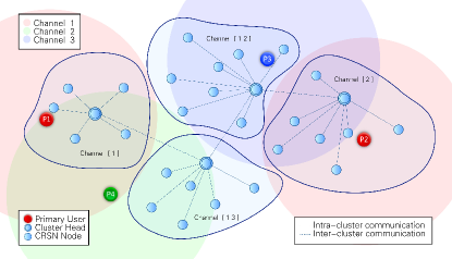
Figure 1: An example of spectrum-aware clustered structure for CRSN

II-B Minimizing Communication Energy

CRSN nodes inherit the energy constraint from traditional WSNs. Therefore, how to properly model and minimize the network-wide communication power becomes our major challenge. We assume that there are $N$ CRSN nodes and $K$ clusters. The $k$th cluster is denoted as $c_{k}$ and has $N_{k}$ CRSN nodes. The $i$th node of $c_{k}$ is $n_{i}^{k}$, whose coordinate is $\left({x_{i},y_{i}}\right)$.

As mentioned before, the power consumption consists of two parts: inter-cluster power communication and intra-cluster communication power. Since all these communications are confined within short distances, free space channel model is applied with $d^{2}$ power loss.

In inter-cluster communication stage, the CH compresses and forwards the collected source information to the sink node through the vacant channels shared with upstream clusters. The inter-cluster power is fixed at maximum to improve network connectivity. The sum power for inter-cluster communication can be expressed as:

$$P_{{\rm{inter}}}=\sum\limits_{k=1}^{K}{P_{{\rm{IC}}}}=KC_{0}P_{r}d_{{\rm{max}}}^{2}$$ (1)

where $C_{0}$ is a loss factor related constant, $P_{r}$ is the minimal receiving power required for successful decoding, and $d_{{\rm{max}}}$ is the maximal transmission range of CRSN node.

Since CH consumes more power than other CRSN nodes, if we fix certain node as CH, its energy will deplete sooner than other nodes. To balance the energy consumption within a cluster, we adopt a CH rotation strategy, which allows all CRSN nodes to take equal probability to become CH.

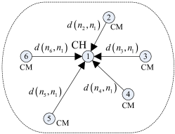
Figure 2: Intra-Cluster Communication

When the $j$th node is selected as CH, all other Cluster Members (CM) report to CH, as shown in Fig. 2. The sum intra-cluster power is:

$$P_{{\rm{intra}}}\left({\rm{CH}}=n_{j}^{k}\right)=\sum\limits_{\scriptstyle i=1\hfill\atop\scriptstyle i\neq j\hfill}^{N_{k}}{P_{t}\left({n_{i}^{k}}\right)}=C_{0}P_{r}\sum\limits_{\scriptstyle i=1\hfill\atop\scriptstyle i\neq j\hfill}^{N_{k}}{d^{2}\left({n_{i}^{k},n_{j}^{k}}\right)}$$ (2)

where $P_{r}$ is the minimal receiving power required, and $d\left({n_{i}^{k},n_{j}^{k}}\right)$ is the Euclidean distance between the $i$th and $j$th node which can be acquired through channel estimation.

Taking into account the fact that all CRSN nodes are equally likely to become CH, the average network-wide intra-cluster communication power can be estimated as:

$$\begin{array}[]{l}P_{{\rm{intra}}}=\sum\limits_{k=1}^{K}{C_{0}\cdot P_{r}\sum\limits_{j=1}^{N_{k}}{\frac{1}{{N_{k}}}}\sum\limits_{\scriptstyle i=1\hfill\atop\scriptstyle i\neq j\hfill}^{N_{k}}{d^{2}\left({n_{i}^{k},n_{j}^{k}}\right)}}\\ =2C_{0}\cdot P_{r}\sum\limits_{k=1}^{K}{\sum\limits_{i=1}^{N_{k}}{d^{2}\left({n_{i}^{k},center\left(k\right)}\right)}}\\ \end{array}$$ (3)

where $center\left(k\right)=\left(\frac{1}{N_{k}}\sum\limits_{i=1}^{N_{k}}{x_{i}^{k}},\frac{1}{N_{k}}\sum\limits_{i=1}^{N_{k}}{y_{i}^{k}}\right)$ is the center of the $k$th cluster.

II-C Optimal Number of Clusters

Now we have $N$ CRSN nodes, and we wish to partition them into $K$ clusters. How many clusters should be created is critical in our energy saving issue. For instance, if $K=N$ i.e. each CRSN node is an independent cluster, and all CRSN nodes act as CHs and have to transmit using maximal power. On the contrary, if $K=1$ i.e. all $N$ CRSN nodes form a single cluster, the intra-cluster communication energy will be too high due to very far intra-cluster distances. Both of these two extreme cases will result in excessive energy consumption. As a result, optimal number of clusters should be carefully chosen to effectively save network-wide energy. For uniformly distributed CRSN nodes, we analytically derive the optimal number of clusters that can statistically minimize the network-wide energy consumption.

From (1) and (3), the expectation of total communication power is:

$$\begin{array}[]{l}P_{{\rm{total}}}=\\ 2C_{0}P_{r}\cdot E\left({\sum\limits_{k=1}^{K}{\sum\limits_{i=1}^{N_{k}}{d^{2}\left({n_{i}^{k},center\left(k\right)}\right)}}}\right)+K\cdot C_{0}P_{r}\cdot d_{{\rm{max}}}^{2}\\ \end{array}$$ (4)

It is reasonable to assume that the randomly deployed CRSN nodes are uniformly distributed in the 2-dimensional area around the center point, and the density $\rho$ is predetermined by application-specific source sensing mission. Therefore:

$$\begin{array}[]{l}E\left({\sum\limits_{k=1}^{K}{\sum\limits_{i=1}^{N_{k}}{d^{2}\left({n_{i}^{k},center\left(k\right)}\right)}}}\right)\\ =N\left({{\mathop{\rm var}}\left({x_{i}^{k}}\right)+{\mathop{\rm var}}\left({y_{i}^{k}}\right)}\right)=\frac{{Nd^{2}}}{6}\\ \end{array}$$ (5)

, where $d$ is the average diameter of a cluster.

Since there are $\frac{N}{K}$ nodes per cluster on average, and the density of CRSN nodes is $\rho$. Then, the area of the cluster can be estimated as $d^{2}=\frac{N}{{K\rho}}$.

Substituting the above formulations into (4), we get:

$$E\left({P_{{\rm{total}}}}\right)=C_{0}P_{r}\left({\frac{{N^{2}}}{{3\rho K}}+Kd_{{\rm{max}}}^{2}}\right)$$ (6)

Obviously, (6) is a convex function and the optimal number of clusters can be estimated by setting its derivative with respect to $K$ to zero. The optimal number of clusters should be rounded to an integer:

$$K_{{\rm{opt}}}=\left\lfloor{\frac{N}{{d_{{\rm{max}}}\sqrt{3\rho}}}+0.5}\right\rfloor$$ (7)

III Energy Efficient Spectrum-Aware Clustering

III-A Groupwise Constrained Agglomerative Clustering

After the optimal number of clusters $K_{{\rm{opt}}}$ is determined, the communication power is only influenced by intra-cluster part. Hence, according to (3), minimizing communication power is equivalent to minimizing sum of squared distance between CRSN nodes and their cluster centers:

$${\rm{mininize}}\ P_{{\rm{total}}}\Leftrightarrow{\rm{mininize}}\ \sum\limits_{k=1}^{K}{\sum\limits_{i=1}^{N_{k}}{d^{2}\left({n_{i}^{k},center\left(k\right)}\right)}}$$ (8)

In clustering analysis theory [15][16], (8) is called sum of squared error (SSE), also known as ‘scatter’. Minimizing SSE is also the goal of many clustering algorithms. Therefore, the energy saving objective coincides with many clustering analysis problems and we can employ the ideas in clustering analysis theory to design desirable clustering schemes. Some computationally feasible heuristic clustering methods have been well developed. The main techniques include K-means, Fuzzy C-means, and Hierarchical Clustering, etc. Several of them are effective in clustering non-cognitive WSNs [12].

However, CRSN nodes should have at least one common available channel to form a cluster. These requirements are imposed on the clustering problem as spectrum-aware constraints, as expressed in (9). Therefore, the existing clustering schemes in non-cognitive WSNs are inapplicable for CRSN, since all of these algorithms do not consider the spectrum-aware constraint.

$$\left|{Chan\left({n_{i}^{k}}\right)\cap Chan\left({n_{j}^{k}}\right)}\right|\geq 1,n_{i}^{k},n_{j}^{k}\in Cluster\left(k\right)$$ (9)

where $\left|{Chan\left({n_{i}^{k}}\right)}\right|$ denotes the number of available channels for $n_{i}^{k}$.

In recent years, a branch of constrained clustering algorithms have been developed to cluster instances with pairwise constraints, such as constrained K-means [13] and constrained complete-link clustering [14]. Pairwise constraints are imposed on pairs of nodes to influence the outcome of clustering algorithm and they mainly include two types: must-link and cannot-link constraints.

As shown in Fig. 3, The must-link constraint forces $n_{i}$ and $n_{j}$ to be in the same cluster, while the cannot-link constraint specifies that $n_{i}$ and $n_{j}$ must not be placed the same cluster. If two CRSN nodes have no available channels in common, they can not be allocated into one cluster, and this is equivalent to imposing cannot-link constraint on this node pair. Thus, the ideas of constrained clustering algorithms can be used to design spectrum-aware clustering scheme for CRSN. However, existing constrained clustering methods can not be directly applied to the spectrum-aware clustering, since our spectrum-aware constraints are imposed on groups, rather than pairs.

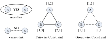
Figure 3: Comparison of Pairwise Constraint and Groupwise Constraint

Now, we define ‘groupwise constraint’ by explaining the differences between ‘pairwise constraint’ and ‘groupwise constraint’. In Fig. 3, three nodes can operate on three channels, and the numbers labeled beside the nodes represent the available channels. On the middle and right, node A and B share channel 1, A and C share channel 2, and B and C share channel 3. If employing pairwise constraint, each node pair shares a common channel and no ‘cannot-link constraint’ is imposed on them, then they can form one cluster. However, if groupwise constraint is imposed, the three nodes share no common channel and can not form a cluster.

The spectrum-aware constraint is a kind of groupwise constraint. All existing pairwise constrained clustering algorithms are iterative, and the basic idea is to satisfy the pairwise constraints in each single iteration. In order to extend the existing algorithms to the model with groupwise constraint, we have to replace pairwise constraint with spectrum-aware groupwise constraint. Here, we impose the spectrum-aware constraint on the complete-link agglomerative clustering algorithm [14] to cluster the CRSN, and name it the ‘Groupwise Constrained Agglomerative Clustering’ (GCAC). The basic idea of GCAC is to set each node as a disjoint cluster at the beginning and then merges two nearest clusters in each iteration until the cluster number reduce to the optimal number. In each iteration, the inter-cluster distances should be re-calculated according to complete-link principle.

III-B Distributed Spectrum-Aware Clustering

Although GCAC can produce clusters satisfying spectrum-aware constraints, it requires some central processor with global node information to perform the clustering algorithm. This is impractical and conflicts with the distributed nature of CRSN. To address this problem, we propose a novel Distributed Spectrum-Aware Clustering (DSAC) protocol which can form clusters in a fully self-organized fashion. The basic idea of DSAC inherits that of GCAC in general: the closest nodes with common channel will agglomerate into a small group first and then the other neighboring nodes will join in one after another. The main differences are as follows: GCAC compares the distance between all clusters and find the global minimum pair to merge first, while DSAC only needs the local minimum distance through neighborhood information exchange and merges the locally closest pair.

DSAC protocol is described by the pseudocode shown in Algorithm 1. It consists of three stages: channel sensing, beaconing and coordination. In channel sensing stage, every CRSN node determines the vacant channels individually and compares it with the previously sensed result. In beaconing stage, CRSN node beacons its node information on the detected vacant channels. If any PU state change is detected, the node declares itself as a new cluster by beaconing a new cluster ID. Otherwise, the node stays with the current cluster. After the node beaconing, the CH updates and beacons the cluster information, including cluster size and common channels. In intra-cluster coordination stage, each node in a cluster first measures the strength of neighboring beacon signals and then announces the pairwise distances. Then, CH determines the inter-cluster distance according to groupwise constraint and complete-link rule [16], in which the distance is jointly decided by the common available channels and the max distance between the nodes of two clusters. In inter-cluster coordination, every CH will send a merge invitation to its nearest neighbor cluster. If any two clusters send merge invitations to each other, they merge into a single cluster by unifying new cluster ID and common channels and selecting a new CH. Otherwise, the cluster just needs to select a new CH while the topology remaining unchanged.

Algorithm 1 Distributed Spectrum-Aware Clustering

  Initialize ()

  Define every node as a disjoint cluster: $c_{i}\left({n_{i}}\right)\Leftarrow n_{i}$

  Channel Sensing ()

  $Chan\left({n_{i}}\right),i\in 1,\cdots,N$

  Distributed Spectrum-Aware Clustering ()

  1. Node Beacon

  for $i\in 1,\cdots,N$ do

     Beacon Node ID

     if $Chan^{t}\left({n_{i}}\right)=Chan^{t-1}\left({n_{i}}\right)$ then

        Beacon Cluster ID: $c_{i}^{t}\left({n_{i}}\right)=c_{i}^{t-1}\left({n_{i}}\right)$

     else

        Beacon New Cluster ID: $c_{i}^{t}\left({n_{i}}\right)={\rm{new\ CID}}$

     end if

  end for

  2. Cluster Beacon:

  for $m\in 1,\cdots,K$ do

     Beacon ClusterSize: $\left|{c_{m}^{t}}\right|$, CommonChannel: $Chan^{t}\left({c_{m}}\right)$

  end for

  3. Intra-cluster Coordinate:

  for $m\in 1,\cdots,K$ do

     if received node beacon number ${\rm{}}c_{n}^{\rm{r}}{\rm{<}}\left|{c_{n}^{t}}\right|$ then

        $d\left({c_{m},c_{n}}\right)\Leftarrow\infty$

     else

        $d\left({c_{m},c_{n}}\right)=\mathop{\max}\limits_{n_{i}\in c_{m},n_{j}\in c_{n}}d\left({n_{i},n_{j}}\right)$

     end if

     Find nearest neighbor cluster:

     $n=\mathop{\arg\min}\limits_{n\in Neighbor\left(m\right)}d\left({c_{m},c_{n}}\right)$

  end for

  4. Inter-cluster Coordinate: $c_{m}$ send merge invitation to $c_{n}$

  if $c_{m}$ also receive merge invitation from $c_{n}$ then

     Unify New Cluster ID: $c_{l}\Leftarrow\left({c_{m},c_{n}}\right)$

     Assign Channel: $Chan\left({c_{l}}\right)=\left|{Chan\left({c_{m}}\right)\cap Chan\left({c_{n}}\right)}\right|$

  end if

  5. Merge Complete: Select new CH

  goto Channel Sensing ()

Fig. 4 shows an example of the DSAC clustering result, where 50 CRSN nodes and 10 PUs are randomly deployed on a 100 meter $\times$100 meter field. There are three available channels in the system (marked by red, green and blue). The clustering result is illustrated by dashed enclosures and the corresponding common channels are labeled in the cluster.

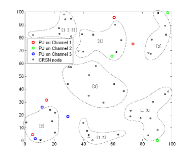
Figure 4: An example of the DSAC clustering result

IV Performance Evaluation

In this section, we analyze and simulate the performance in terms of scalability, energy consumption and stability. We employ Monte Carlo experiments and repeat a hundred thousand times to compute the target value.

In order to evaluate the performance of the proposed DSAC scheme, we have to employ a generally accepted algorithm called K-means clustering as a reference. According to literature, K-means can converge to local minimal SSE in very short time. Although K-means does not include the spectrum-aware constraint and is only applicable for non-cognitive WSNs, it serve as a good criterion for performance evaluation.

For all the experiments, we randomly deploy PUs and CRSN nodes in a $100\times 100$ square meters area. The PUs can operate on three channels, and CRSN nodes can only access the channels on which the neighboring PUs are inactive. Every PU randomly occupies one of the three channels. The protection range for PU is 20 meters, which means the PU’s CRSN neighbors within this range can not access its occupied channel.

For GCAC algorithm, the time complexity is similar to the existing complete-link agglomerative clustering algorithms, which is $O(N^{2}\log N)$[16]. Although this complexity is much lower than the exhaustive method and can be well implemented in some small sensor networks, it is still too high to be implemented in the large scale CRSN. Relatively, the time complexity of K-means is much lower, which is $O(NK)$.

In the first experiment, we simulate the average converge time of the three clustering schemes when CRSN size is growing. As shown in Fig. 5, the converging time of GCAC grows proportionally with the CRSN size, while the DSAC converges almost as fast as the efficient K-mean algorithm. This result shows DSAC has similar time complexity to K-means and therefore exhibits satisfying scalability.

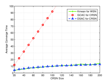
Figure 5: Scalability: CRSN size vs converge time

For the following experiments, we assume the max transmission range for CRSN node is 50 meters, and 20 CRSN nodes and 5 PU nodes are uniformly distributed in the same area. According to the theoretical analysis in Section II.C, the estimated optimal cluster number is about five. In the simulation, we set the cluster number from 3 to 8, and calculate the average power consumed by CRSN nodes. From Fig. 6, we find that the minimum power occurs when cluster number is about 5 to 6, and this result agrees well with the theoretical analysis.

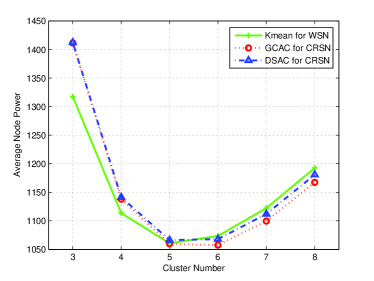
Figure 6: Comparison of average energy among three schemes

To evaluate the influence of PUs on clustering, we simulate the average CRSN node power consumption when different numbers of PU node are active. In Fig. 7, we set the CRSN size as 30 and adjust the PU number from 1 to 10. For non-cognitive WSN, the K-means clustering result is not influenced by PU systems, therefore the average node power keeps steady. For CRSN, as more PU nodes are active, more spectrum-aware constraints are imposed on the clustering process. Therefore the clustering results are poorer in terms of energy consumption. Again, we find the performance of DSAC only to be slightly worse than that of GCAC.

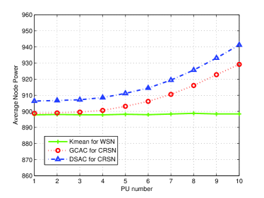
Figure 7: PU number vs average node power

In the final experiment, we examine the proposed algorithm’s stability under dynamic PU activities. For exhaustive search method, K-means and GCAC, if any PU activity or CRSN node position changed, the whole network should be involved in re-clustering, which makes the network topology less stable and requires extra control overhead. However, in DSAC, only the nodes that detect PU activity change will engage in re-clustering. In Fig. 8, when one PU changes its status, only 3 of 50 CRSN nodes are affected. After two merges, the network once again converges to stable topology, which is much faster than GCAC. During the re-clustering, the rest nodes’ status and their clustering structure remain the same. Their application-specific sensing task won’t be influenced. Hence, the stability of network is preserved as much as possible.

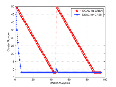
Figure 8: Comparison of dynamic stability between GCAC and DSAC

V Conclusion

In this paper, we proposed a novel distributed spectrum-aware clustering scheme for cognitive radio sensor networks. We modeled the communication power for CRSN, which consists of intra-cluster aggregation and inter-cluster relaying. After deriving the optimal number of clusters, we minimize the CRSN energy using groupwise constrained clustering, in which the spectrum-aware requirement is regarded as groupwise constraint. With the proposed DSAC protocol, desirable clustering results can be produced. Through extensive simulations, we find that DSAC has preferable scalability and stability because of its low complexity and quick convergence under dynamic PU activity change.

References

- [1] O. Akan, O. Karli, O.Ergul, and M. Haardt, “Cognitive radio sensor networks,” IEEE Network, vol.23, no.4, pp.34-40 July 2009.
- [2] A. S. Zahmati, S. Hussain, X. Fernando, and A. Grami, “Cognitive Wireless Sensor Networks: Emerging topics and recent challenges,” Proc. IEEE TIC-STH, pp.593-596 Sept. 2009.
- [3] Vijay G., Bdira E., and Ibnkahla M. “Cognitive approaches in Wireless Sensor Networks: A survey,” Proc. QBSC, pp.177-180, May 2010.
- [4] H. Zhang, Z. Zhang, Y. Chau, “Distributed compressed wideband sensing in Cognitive Radio Sensor Networks,” in Proc. IEEE INFOCOM WKSHPS, April 2011.
- [5] K.-L.A. Yau, P. Komisarczuk, P.D. Teal, “Cognitive Radio-based Wireless Sensor Networks: Conceptual design and open issues,” Proc. LCN, pp.955-962, Oct. 2009.
- [6] H. Zhang, Z. Zhang, X. Chen and R. Yin, “Energy Efficient Joint Source and Channel Sensing in Cognitive Radio Sensor Networks,” in Proc. IEEE ICC, June 2011.
- [7] T. Chen, H. Zhang, G. M. Maggio, I. Chlamtac, “Topology Management in CogMesh: A Cluster-Based Cognitive Radio Mesh Network,” Proc. IEEE ICC 2007, pp. 6516-6521, June 2007.
- [8] K. E. Baddour, O. Ureten, T. J. Willink, “Efficient Clustering of Cognitive Radio Networks Using Affinity Propagation,” Proc. IEEE ICCCN 2009, pp. 1-6, Aug. 2009.
- [9] F. Xu, L. Zhang, Z. Zhou, Y. Ye, “Spectrum-aware Location-based Routing in Cognitive UWB network,” Proc. CrownCom 2008, pp. 1, May 2008.
- [10] W. B. Heinzelman, A. P. Chandrakasan, H. Balakrishnan, “An application-specific protocol architecture for wireless microsensor networks,” IEEE Transaction on Wireless Communications, vol.1, no.2, pp.660-670, Oct. 2009.
- [11] O. Younis, S. Fahmy, “HEED a hybrid, energy-efficient, distributed clustering approach for ad hoc sensor networks,” IEEE Transaction on Mobile Computing, vol.3, no.4, pp.366-379, Oct.-Dec. 2004
- [12] D. C. Hoang, R. Kumar, S. K. Panda, “Fuzzy C-Means clustering protocol for Wireless Sensor Networks,” Proc. IEEE ISIE 2010, pp. 3477 - 3482, July 2010.
- [13] K. Wagstaff, C. Cardie, S. Rogers, S. Schroedl, “Constrained K-means Clustering with Background Knowledge,” Proc. ICML 2001, pp. 577-584, 2001.
- [14] D. Klein, S. D. Kamvar, C. D. Manning, “From Instance-level Constraints to Space-level Constraints: Making the Most of Prior,” Proc. ICML 2002, pp. 307-314, 2002.
- [15] A. K. Jain, R. C. Dubes, “Algorithms for clustering data,” Prentice-Hall, 1988.
- [16] P. N. Tan, M. Steinbach, V. Kumar, “Introduction to Data Mining: Chapter 8. Cluster Analysis: Basic Concepts and Algorithms,” Pearson Addison Wesley, 2006.