Energy Efficient Joint Source and Channel Sensing in Cognitive Radio Sensor Networks

Abstract

A novel concept of Joint Source and Channel Sensing (JSCS) is introduced in the context of Cognitive Radio Sensor Networks (CRSN). Every sensor node has two basic tasks: application-oriented source sensing and ambient-oriented channel sensing. The former is to collect the application-specific source information and deliver it to the access point within some limit of distortion, while the latter is to find the vacant channels and provide spectrum access opportunities for the sensed source information. With in-depth exploration, we find that these two tasks are actually interrelated when taking into account the energy constraints. The main focus of this paper is to minimize the total power consumed by these two tasks while bounding the distortion of the application-specific source information. Firstly, we present a specific slotted sensing and transmission scheme, and establish the multi-task power consumption model. Secondly, we jointly analyze the interplay between these two sensing tasks, and then propose a proper sensing and power allocation scheme to minimize the total power consumption. Finally, simulation results are given to validate the proposed scheme.

I Introduction

Wireless Sensor Networks (WSN) are capable of monitoring physical or environmental information (e.g. temperature, sound, pressure), and collecting them to certain access points according to various applications. The extensive deployment of WSN has changed our lives dramatically. However, current WSN nodes usually operate on license-exempt Industrial, Scientific and Medical (ISM) frequency bands [1], and these bands are shared with many other successful systems such as Wi-Fi and Bluetooth, causing severe spectrum scarcity problems [2]. To deal with such problems, a new sensor networking paradigm of Cognitive Radio Sensor Network (CRSN) which incorporates cognitive radio capability on the basis of traditional wireless sensor networks was introduced [3]. CRSN nodes operate on licensed bands and can periodically sense the spectrum, determine the vacant channels, and use them to report the collected source information. The main design principles and features of CRSNs are discussed openly in literature [1]-[4]. According to these literatures, CRSN enjoys many advantages, such as efficient spectrum usage, flexible deployment and good radio propagation property. However, WSN nodes are low cost and usually equipped with a limited energy source, such as a battery, and CRSN nodes also inherit this fundamental limitation. What s more, the CRSN node bears one more task of spectrum sensing, and this task also consumes energy. This fact makes the energy scarcity problem in CRSN even more severe. Hence, how to minimize the total energy consumption for CRSN node and thus make the system the most energy efficient has become an urgent problem.

In our viewpoint, there are two basic types of sensing tasks for the CRSN node, one is Application-Oriented Source Sensing (AppOS) and the other is Ambient-Oriented Channel Sensing (AmOS). By source sensing we mean the process of collecting source information (e.g. temperature, sound) and delivering it to the Access Point (AP), and by channel sensing we mean the process of periodically sensing the ambient radio environment and determining the vacant channels for opportunistic spectrum access.

The energy saving problems of both AppOS and AmOS have been investigated separately in existing literature. The energy consumption models for AppOS have been established in the context of conventional WSN. The energy-distortion tradeoffs in energy-constrained sensor networks is investigated in [7], and energy efficient lossy transmission for wireless sensor networks is studied in [8], for Gaussian sources and unlimited bandwidth. Another issue of energy efficient AmOS has also been studied separately, in the cognitive radio scenario. Maleki has designed a sleep/censor scheme to reduce spectrum sensing energy [9]. Su and Zhang proposed an energy saving spectrum sensing scheme by adaptively adjusting the spectrum sensing periods utilizing PU’s activity patterns [10]. [11] studied the influence of sensing time on the probability of detection and probability of false alarm.

However, the unique mechanism of CRSN is that every CRSN node performs AppOS and AmOS at the same time. This requires us to consider the resource saving problems of AppOS and AmOS jointly. In order to prolong the lifespan, there is a need to properly distribute limited power into these two concurrent tasks. On one hand, if we put excessive power into AppOS, the resources left for AmOS will be diminished. We can obtain more precise and unaffected application-specific source information. But, due to the lack of channel resource information, acquired source information can not be delivered timely and effectively to AP. Furthermore, the probability of miss detection of Primary Signals can be prominently high. It will cause interference to the underlying Primary System. On the other hand, if we put too much power into AmOS, we can obtain enough reliable channel access opportunities, and reduce the interference to the Primary System. Vice versa, the power left for AppOS is not enough for delivering source information at a coding rate capable of meeting the distortion requirement despite the implementing of distributed source coding in the sensor network. Therefore, our paper mainly aims at tackling this joint energy saving problem, which has not been considered before. The main contributions of our work are as follows: we jointly model the power consumption of AmOS and AppOS and use the transmission probability to bond these two interrelated tasks; we find that within bounded distortion, there is always a minimal total power consumption and corresponding power allocation scheme for the CRSN system, which is the most power efficient solution.

The rest of this paper is organized as follows. In Section II, we make basic assumptions about the CRSN, and provide a brief introduction of the considered system. In Section III, we give detailed models and jointly analyze the power consumption of AppOS and AmOS. Then, several simulation results are presented in Section IV to further validate our analysis. Finally, the whole paper is concluded in Section V.

II System Model

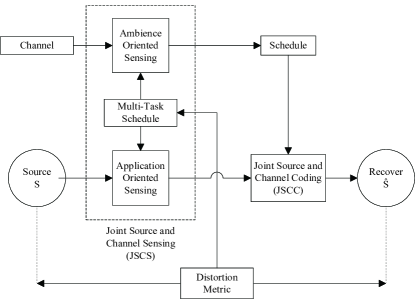
Figure 1: An overview of the considered system model.

In this paper, we consider the Multi-task Sensing architecture in CRSN nodes, as shown in Fig.1. We observe two dominating features of the considered CRSN:

Feature 1: In a CRSN node, two major tasks need to be modeled as follows:

1. Application Oriented Source Sensing (AppOS)

   We define source sensing as the process of collecting various source information (e.g. temperature, pressure, position, etc.) according to the application-specific demand and delivering it to the Access Point (AP). The main objective of AppOS is realizing accurate acquisition of the source information.

2. Ambient Oriented Channel Sensing (AmOS)

   Channel sensing is the process of periodically sensing the ambient radio environment by means of spectrum sensing and energy detection. It, thus, determines the vacant channels for opportunistic spectrum access or perceives energy distribution of surrounding nodes for cooperation. The main objective of AmOS is to realize effective and efficient exploration of spectrum resources.

Feature 2: As a characteristic inherited from the traditional WSN, every CRSN node is power-constrained due to limited energy supply. Both AmOS and AppOS consume energy. We have to save as much energy as possible while delivering the source information to AP within bounded distortion.

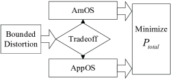
Figure 2: The interplay between the two tasks.

Fig.2 depicts the subtle interplay between AppOS and AmOS sensing under the interference, distortion and power resource constraint. It’s like you have two ears listening to two distinct but related objects in a noisy environment. On the one hand, your left ear listens to the monitored source, trying to hear the most undistorted sound. On the other hand, your right ear listens to the slight ambient sound on the radio spectrum, because you are not allowed to speak when others talk. Our goal is to optimally balance the two ears and make them the most efficient.

II-A Slotted Sensing and Transmission Scheme

We present a specific sensing and transmission scheme below in Fig.3:

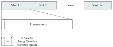
Figure 3: Slotted sensing and transmission scheme.

Every node partitions the time domain into periods, namely slots, of equal length $T$. At the beginning of each slot, the cognitive sensor node makes a decision on whether or not to transmit based on the $N$ samples energy detection spectrum sensing result. The spectrum sensing is always performed ahead of the data transmission. In our scheme, we should point out three basic assumptions:

AS1: Both spectrum sensing and data transmission consume energy. And the total energy is limited in one CRSN node.

AS2: The slot length $T$ is short enough, so that the status of primary user activity remains the same during one slot.

AS3: The time period of spectrum sensing is rather short compared with transmission period and thus can be omitted.

In the following sections, we will establish detailed models for both sensing tasks and analyze the power consumption tradeoff between them.

III Energy Efficient Joint Source and Channel Sensing

In this section, the relationships between power consumption and performances are discussed. We present specific models for both AmOS and AppOS, and then jointly analyze the relationship and tradeoff between them. We prove that optimal power allocation scheme can indeed be obtained.

III-A AmOS: Energy Detection based Spectrum Sensing

In recent years, many methods have been developed for spectrum sensing, including matched filter detection, energy detection and cyclostationary feature detection. Among them, energy detection is the most popular spectrum sensing scheme. It is the most suitable for CRSN node due to its simplicity of hardware implementation and low signal processing cost. Therefore, we choose energy detection as our spectrum sensing technique for CRSN node.

We assume that the CRSN node operates at certain carrier frequency $f_{c}$ with bandwidth $W$, and samples the signal within this range $N$ times per slot.

The discrete signal that the CRSN node receives can be represented as:

$$y\left(n\right)=\left\{{\begin{array}[]{*{20}c}{s\left(n\right)+u\left(n\right),\quad{\cal H}_{1}:{\rm{primary\;user\;is\;active}}}\\ {u\left(n\right),\quad\quad\quad{\cal H}_{0}:{\rm{primary\;user\;is\;inactive}}}\\ \end{array}}\right.$$ (1)

The primary signal $s(n)$ is independent, identically distributed (i.i.d) random process with zero mean and variance $E\left[{\left|{s(n)}\right|^{2}}\right]=\sigma_{s}^{2}$, and the noise $u(n)$ is i.i.d random process with zero mean and variance $E\left[{\left|{u(n)}\right|^{2}}\right]=\sigma_{u}^{2}$. We assume that the primary signal $s(n)$ is MPSK complex signal, and the noise $s(n)$ is complex Gaussian.

As the performance criteria for the proposed spectrum sensing method, the two important parameters worth mentioning are: probability of detection and probability of false alarm. The probability of detection, denoted as $P_{D}$, is the probability that the CRSN node successfully detects the primary user when it’s active, under hypothesis $\mathcal{H}_{1}$. The probability of false alarm, denoted as $P_{FA}$, is the probability that the CRSN node falsely determines the presence of primary signal when the primary user is actually inactive, under hypothesis $\mathcal{H}_{0}$.

The energy detector is as follows:

$$T(y)=\frac{1}{N}\sum\limits_{n=1}^{N}{\left|{y(n)}\right|^{2}}$$ (2)

According to the Central Limit Theorem, the statistics $T(y)$ is approximately Gaussian distributed when $N$ is large enough under both hypothesis $\mathcal{H}_{1}$ and $\mathcal{H}_{0}$. The probability density function(PDF) of statistics $T(y)$ can be expressed as:

$$T(y)\sim\left\{{\begin{array}[]{*{20}c}{\mathcal{N}\left({\mu_{0},\sigma_{0}^{2}}\right),{\rm{\ \ \ under\ \ \mathcal{H}_{0}}}}\\ {\mathcal{N}\left({\mu_{1},\sigma_{1}^{2}}\right),{\rm{\ \ \ under\ \ \mathcal{H}_{1}}}}\\ \end{array}}\right.$$ (3)

When the primary signal $s(n)$ is MPSK complex signal, and the noise $s(n)$ is complex Gaussian [11], we can derive the probability of false alarm:

$$P_{FA}\left({\varepsilon,N}\right)=Q\left({(\frac{\varepsilon}{{\sigma_{u}^{2}}}-1)\sqrt{N}}\right)$$ (4)

where $Q\left(x\right)=\frac{1}{{2\pi}}\int_{x}^{\infty}{\exp(-\frac{{t^{2}}}{2})dt}$ is the tail probability of the standard normal distribution (also known as the Q function).

For certain threshold $\varepsilon$, the probability of detection can be expressed as:

$$P_{D}\left({\varepsilon,N}\right)=Q\left({(\frac{{\varepsilon-\sigma_{s}^{2}}}{{\sigma_{u}^{2}}}-1)\sqrt{\frac{N}{{2\sigma_{s}^{2}/\sigma_{u}^{2}+1}}}}\right)$$ (5)

Since the slot period $T$ is short enough, we can assume that the primary user activity keeps unchanged during a single slot.

When the CRSN node fails to detect the PU signal, its signal will collide with the primary user signal and bring interference into the PU system. We denote $P_{E}=1-P_{D}$ as the probability of missed detection, and have the following assumption:

AS4: There is a maximal missed detection probability that the PU system can tolerate, and a typical value for this parameter is 0.1 [12]. $P_{E}$ should be smaller than this value.

Because $Q\left(\cdot\right)$ is monotonically decreasing, we find that the probability of false alarm drops as the sample number $N$ increases:

$$P_{FA}=Q\left({\sqrt{2\sigma_{s}^{2}/\sigma_{u}^{2}+1}Q^{-1}\left({1-P_{E}}\right)+\sqrt{N}\sigma_{s}^{2}/\sigma_{u}^{2}}\right)$$ (6)

The resulted probability that the CRSN node is allowed to transmit is:

$$\begin{array}[]{*{20}c}{p^{\prime}_{t}=\left({1-P_{FA}}\right)p({\rm{H}}_{0})+\left({1-P_{D}}\right)p({\rm{H}}_{1})}\\ {\begin{array}[]{*{20}c}{=\left({1-Q\left({\sqrt{\frac{{2\sigma_{s}^{2}}}{{\sigma_{u}^{2}}}+1}Q^{-1}\left({1-P_{E}}\right)+\sqrt{N}\frac{{\sigma_{s}^{2}}}{{\sigma_{u}^{2}}}}\right)}\right)}\\ {\times p({\rm{H}}_{0})+P_{E}p({\rm{H}}_{1})}\\ \end{array}}\\ \end{array}$$ (7)

where $p({\rm{H}}_{0})$ and $p({\rm{H}}_{1})$ are the inactive and active probabilities of the primary user, respectively. Leaving out the collision probability $P_{C}=P_{E}p({\rm H}_{1})$, we can obtain the effective transmission probability available for CRSN node:

$$\begin{array}[]{l}p_{t}=p^{\prime}_{t}-P_{E}p({\rm{H}}_{1})\\ =\left({1-Q\left({\sqrt{\frac{{2\sigma_{s}^{2}}}{{\sigma_{u}^{2}}}+1}Q^{-1}\left({1-P_{E}}\right)+\sqrt{N}\frac{{\sigma_{s}^{2}}}{{\sigma_{u}^{2}}}}\right)}\right)p({\rm{H}}_{0})\\ \end{array}$$ (8)

Denoting the energy consumed in one sample as $E_{sample}$, the average AmOS power consumption can be expressed as:

$$P_{{}_{AmOS}}=\frac{{E_{sample}\times N}}{T}$$ (9)

Rewriting the AmOS power expression with respect to the effective transmission probability $p_{t}$ gives:

$$\begin{array}[]{l}P_{{}_{AmOS}}\left({p_{t}}\right)\\ =\left({\frac{{Q^{-1}\left({1-\frac{{p_{t}}}{{p({\rm{H}}_{0})}}}\right)-\sqrt{\frac{{2\sigma_{s}^{2}}}{{\sigma_{u}^{2}}}+1}Q^{-1}\left({1-P_{E}}\right)}}{{\sigma_{s}^{2}/\sigma_{u}^{2}}}}\right)^{2}\times\frac{{E_{sample}}}{T}\\ \end{array}$$ (10)

Note that (10) is valid only when $p_{t}$ falls in the range of:

$$\left({1-Q\left({\sqrt{\frac{{2\sigma_{s}^{2}}}{{\sigma_{u}^{2}}}+1}Q^{-1}\left({1-P_{E}}\right)}\right)}\right)p({\rm{H}}_{0})<p_{t}<p({\rm{H}}_{0})$$ (11)

When $0<p_{t}<\left({1-Q\left({\sqrt{\frac{{2\sigma_{s}^{2}}}{{\sigma_{u}^{2}}}+1}Q^{-1}\left({1-P_{E}}\right)}\right)}\right)p({\rm{H}}_{0})$, the transmission probability is so small that the requirement of AS4 can always be met. In this case, we don’t have to do any spectrum sensing, and $P_{{}_{AmOS}}\left({p_{t}}\right)=0$.

III-B AppOS: Distortion-Constrained Source Sensing

In this subsection, we step forward to explore the connection between $p_{t}$ and average AppOS power $P_{{}_{AppOS}}$. We model the power consumption of the AppOS task, which comprises the target sensing application, source-channel coding and transmission.

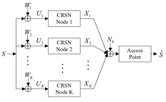
Figure 4: Gaussian cognitive radio sensor network.

As shown in Fig.4, we consider the Gaussian source $S$ with zero mean and variance $\sigma_{S}^{2}$. The source generates symbols at a constant rate $L$ symbols per second. Every CRSN node’s observation includes a Gaussian noise $W_{i}$ with zero mean and equal variance $\sigma_{W}^{2}$. The source $S$ is finally recovered as $\hat{S}$ at the Access Point(AP).

Every CRSN node first compresses its observation, then transmit it to AP over the MAC using independently generated channel codes. This is a multiterminal source coding system, and can be classified as the CEO problem. For the symmetric Gaussian CEO problem, the $K$ nodes rate-distortion function [6] is:

$$R_{source}\left(D\right)=\frac{L}{2}\log_{2}\left({\frac{{\left({\frac{{\sigma_{S}^{2}}}{D}}\right)^{\frac{1}{K}}}}{{1-\frac{{\sigma_{W}^{2}}}{K}\left({\frac{1}{D}-\frac{1}{{\sigma_{S}^{2}}}}\right)}}}\right)$$ (12)

Note that we will only use the Gaussian source for illustration later. For other sources, explicit form of the rate-distortion function hasn’t been derived. However, the outer bound can be obtained, which is exactly in the form of (12) [6]. The outer bound represents the worst case, which means for a given source variance $\sigma_{S}^{2}$, the Gaussian sources are the most difficult to compress.

We assume that the communication channel of interest is AWGN channel. According to the Shannon Channel Capacity Theorem:

$$R_{channel}\leq W\log_{2}\left\{{1+\frac{P}{{N_{0}W}}}\right\}$$ (13)

where $W$ is the channel bandwidth, and $N_{0}$ is the unilateral noise power spectral density. The energy for correctly delivering of every bit of source information is:

$$E_{bit}=\frac{P}{R}=N_{0}W\frac{{2^{\frac{{R_{channel}}}{W}}-1}}{{R_{channel}}}$$ (14)

Thus, the average AppOS power consumption can be expressed as:

$$\begin{array}[]{l}P_{{}_{AppOS}}=p^{\prime}_{t}E_{bit}R_{channel}\\ =p^{\prime}_{t}N_{0}W\left({2^{\frac{{R_{channel}}}{W}}-1}\right)\\ \end{array}$$ (15)

We should point out that the source is encoded at rate $R_{source}$. And $R_{source}$ is determined by the distortion $D$, the number of nodes $K$, the variance of source $\sigma_{S}^{2}$ and the variance of noise $\sigma_{W}^{2}$, regardless of the PU activity.

However, only a fraction of $p_{t}$ throughout the time domain can be used for effective transmission. Therefore, in order to offset the slots forbidden for transmission, the channel coding rate should be higher than source coding rate:

$$\begin{array}[]{l}R_{channel}=\frac{{R_{source}}}{{p_{t}}}\\ =\frac{L}{{2p_{t}}}\log_{2}\left(\frac{{\left({\frac{{\sigma_{S}^{2}}}{D}}\right)^{\frac{1}{K}}}}{{1-\frac{{\sigma_{W}^{2}}}{K}\left({\frac{1}{D}-\frac{1}{{\sigma_{S}^{2}}}}\right)}}\right)\\ \end{array}$$ (16)

From (8), (15) and (16), we formulate the average AppOS power with respect to $p_{t}$:

$$\begin{array}[]{l}P_{{}_{AppOS}}\left({p_{t}}\right)=\left({p_{t}+P_{E}p({\rm H}_{1})}\right)N_{0}W\\ \times\left({\left(\frac{{\left({\frac{{\sigma_{S}^{2}}}{D}}\right)^{\frac{1}{K}}}}{{1-\frac{{\sigma_{W}^{2}}}{K}\left({\frac{1}{D}-\frac{1}{{\sigma_{S}^{2}}}}\right)}}\right)^{\frac{L}{{2p_{t}W}}}-1}\right)\\ \end{array}$$ (17)

Proposition 1: $P_{{}_{AppOS}}\left({p_{t}}\right)$ is a monotonically decreasing function.

Proof: See Proof of Proposition 1 in Appendix B

The result can be confusing at the first glance, since we may intuitively think that the AppOS power would grow with the transmission probability. However, this is not the case. Now we provide a heuristic understanding. If the transmission probability $p_{t}$ is very low, the channel coding rate in the transmitting slots has to be very high to make up for those silent slots. According to (14), the transmission becomes less power efficient. Therefore, for certain distortion and source coding rate, the average AppOS power decreases with $p_{t}$.

III-C Joint Power Consumption Model

On the one hand, if we allocate more power for AmOS, we are more confident about the status of the primary user, therefore we can grasp more opportunities for transmission. On the other hand, delivering the information of the target source to the AP also requires energy; the more power we allocate to AppOS, the higher source and channel coding rate we can achieve. Under the condition that power is constrained in CRSN node, we face a dilemma on how to balance the two tasks. The effective transmission probability $p_{t}$ is the key parameter that naturally connects the two sensing tasks.

From (10) and (17), the total power consumption can be modeled as a function of $p_{t}$:

$$\begin{array}[]{l}P_{total}\left({p_{t}}\right)\\ =\left({\frac{{Q^{-1}\left({1-\frac{{p_{t}}}{{p({\rm H}_{0})}}}\right)-\sqrt{\frac{{2\sigma_{s}^{2}}}{{\sigma_{u}^{2}}}+1}Q^{-1}\left({1-P_{E}}\right)}}{{\sigma_{s}^{2}/\sigma_{u}^{2}}}}\right)^{2}\times\frac{{E_{sample}}}{T}+\\ \left({p_{t}+P_{E}p({\rm H}_{1})}\right)N_{0}W\left({\left(\frac{{\left({\frac{{\sigma_{S}^{2}}}{D}}\right)^{\frac{1}{K}}}}{{1-\frac{{\sigma_{W}^{2}}}{K}\left({\frac{1}{D}-\frac{1}{{\sigma_{S}^{2}}}}\right)}}\right)^{\frac{L}{{2p_{t}W}}}-1}\right)\\ \end{array}$$ (18)

Proposition 2: When the probability of false alarm $P_{FA}<\frac{1}{2}$, $P_{total}\left({p_{t}}\right)$ is a convex function with respect to $p_{t}$. That is to say, we can obtain the minimal total power consumption and a unique power efficient allocation solution for the CRSN node, if $P_{FA}$ falls into this range.

Proof: See Proof of Proposition 2 in Appendix A

Theorem 1: Under our slotted sensing and transmission scheme, there is always a minimal total power consumption and corresponding optimal power allocation scheme for the CRSN to achieve certain distortion constraint.

Proof: See Proof of Theorem 1 in Appendix B

We end this section by summarizing the above results. In the cases when $P_{FA}<\frac{1}{2}$, we know $P_{total}\left({p_{t}}\right)$ is convex from Proposition 1. We can thus design efficient search algorithm to find the optimal power consumption. Otherwise, Theorem 1 shows that, though the function is not convex, we can still find the optimal power consumption through exhaustive search, and calculate the corresponding power allocation scheme.

IV Simulation Result

To validate the analysis of the proposed energy efficient Joint Source and Channel Sensing scheme, we present several numerical results. We use Matlab as our simulator. For all scenarios, we set the PU occupation rate to be $0.3$, which means the PU is active with this probability. The max miss detection probability in AS4 is $0.1$; the energy consumed per sample in spectrum sensing is $E_{sample}=0.1$mW; the source is of unit variance, i.e. $\sigma_{S}^{2}=1$; the symbol rate of the source is $L=1$M bauds; the distortion is constrained to be 0.1. There are $K=10$ nodes and the bandwidth of the considered AWGN channel is $W=5$MHz.

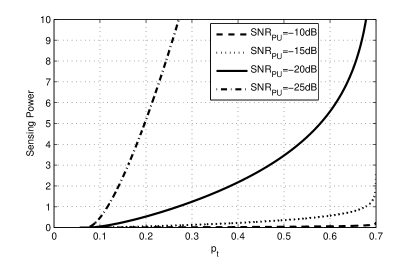
Figure 5: Average AmOS power under different PU SNR.

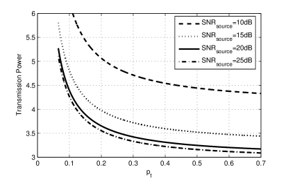
Figure 6: Average AppOS power under different source SNR.

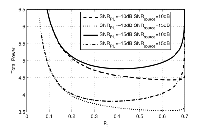
Figure 7: Average total power under different PU SNR and source SNR.

From Fig.5, we find that the average AmOS power increases with the effective allowed transmission probability, i.e. the more we pay on spectrum sensing, the more chances we obtain for transmission. We can see from Fig.6 that the average AppOS power drops as transmission probability increases, and this is consistent with the analysis of Proposition 1. Fig.5 and Fig.6 also show that as the spectrum environment and monitored source become noisier, the corresponding AmOS and AppOS power consumption increase.

Finally, Fig.7 shows that there is a unique valley point in every curve, which corresponds to the optimal total power. Any other transmission probability and power allocation scheme will result in a higher total power consumption. In Fig.7, when the source SNR is $10$dB and the PU SNR is $-15$dB, the optimal $p_{t}$ is $0.42$, and the optimal total power is $4.8$W. $5.1\%$ of the power should be allocated to AmOS to achieve optimality.

V Conclusion

In this paper, we introduced a novel concept of Joint Source and Channel Sensing for Cognitive Radio Sensor Networks, which seeks to deliver the application source information to the access point in a most power efficient manner. We presented a specific slotted sensing and transmission scheme. By exploiting the relation between AmOS and AppOS tasks, we modeled their power consumption properly and jointly analyzed them. We proved that optimal power consumption and corresponding power allocation scheme exist for fixed distortion requirement. Finally, we present simulation results to support our analysis.

VI Appendix A: Proof of Proposition 2

Proof: The former part of (18) can be viewed as a composite function $h\left({p_{t}}\right){\rm{}}={\rm{}}g\left({f\left({p_{t}}\right)}\right)$, where $f\left({p_{t}}\right)=Q^{-1}\left({1-\frac{{p_{t}}}{{p({\rm{H}}_{0})}}}\right)$, and

$$g\left(x\right)=\left({\frac{{x-\sqrt{\frac{{2\sigma_{s}^{2}}}{{\sigma_{u}^{2}}}+1}Q^{-1}\left({1-P_{E}}\right)}}{{\sigma_{s}^{2}/\sigma_{u}^{2}}}}\right)^{2}\times\frac{{E_{sample}}}{T}$$ (19)

Since$f\left({p_{t}}\right)-\sqrt{\frac{{2\sigma_{s}^{2}}}{{\sigma_{u}^{2}}}+1}Q^{-1}\left({1-P_{E}}\right)=\sqrt{N}\frac{{\sigma_{s}^{2}}}{{\sigma_{u}^{2}}}>0$, and all other parameters in $g(x)$ are non-negative, $g(x)$ is a convex and non-decreasing function.

According to the property of inverse Q function, $f(p_{t})$ is convex as long as $p_{t}>\frac{1}{2}p\left({H_{0}}\right)$, which is equivalent to $P_{FA}<\frac{1}{2}$.

Now that $f\left(\cdot\right)$ and $g\left(\cdot\right)$ are convex functions and $g\left(\cdot\right)$ is non-decreasing, then the former part $h(x)=g(f(x))$ is convex.

The latter part of (18) can prove to be convex through its second order derivative:

$$\begin{array}[]{l}\frac{{\partial^{2}P_{{}_{AppOS}}}}{{\partial p_{t}^{2}}}=\\ \frac{{LN_{0}\ln\left(C\right)C^{\frac{L}{{2p_{t}W}}}\left({L\ln\left(C\right)\left({p_{t}+P_{E}p\left({H_{1}}\right)}\right)+4p_{t}WP_{E}p\left({H_{1}}\right)}\right)}}{{4p_{t}^{4}W}}\\ \end{array}$$ (20)

where $C=\frac{{\left({\frac{{\sigma_{S}^{2}}}{D}}\right)^{\frac{1}{K}}}}{{1-\frac{{\sigma_{W}^{2}}}{K}\left({\frac{1}{D}-\frac{1}{{\sigma_{S}^{2}}}}\right)}}>1$, and all other parameters are positive. Obviously (20) is positive, thus the latter part of (18) is also convex.

The sum power $P_{total}\left({p_{t}}\right)$, as the sum of two convex functions, is convex.

VII Appendix B: Proof of Theorem 1

Proof: The derivative of $P_{{}_{AppOS}}$ is:

$$\begin{array}[]{l}P^{\prime}_{{}_{AppOS}}\left({p_{t}}\right)=\\ -\frac{{\left({\left({L\left({1+p\left({H_{1}}\right)}\right)\ln C-2p_{t}W}\right)C^{\frac{L}{{2p_{t}W}}}+2p_{t}W}\right)N_{0}}}{{2p_{t}}}\\ \end{array}$$ (21)

After observing (21), we can easily find that $P^{\prime}_{{}_{AppOS}}\left({0^{+}}\right)=-\infty$ and $P^{\prime}_{{}_{AppOS}}\left({+\infty}\right)=0$. Given that (24) is positive, we can conclude that $P^{\prime}_{{}_{AppOS}}\left({p_{t}}\right)<0$, and $P_{{}_{AppOS}}\left({p_{t}}\right)$ is monotonically decreasing. Thus Proposition 1 is proved.

When $p_{t}$ falls in the range of (11),

$$\begin{array}[]{l}P_{{}_{AmOS}}^{\prime}\left({p_{t}}\right)=\frac{{2E_{sample}}}{T}Q^{-1}\left({1-\frac{{p_{t}}}{{p({\rm{H}}_{0})}}}\right)^{\prime}\times\\ \left({\frac{{Q^{-1}\left({1-\frac{{p_{t}}}{{p({\rm{H}}_{0})}}}\right)-\sqrt{\frac{{2\sigma_{s}^{2}}}{{\sigma_{u}^{2}}}+1}Q^{-1}\left({1-P_{E}}\right)}}{{\sigma_{s}^{2}/\sigma_{u}^{2}}}}\right)\\ \end{array}$$ (22)

It can be verified from (21) and (22) that

$$\begin{array}[]{l}P^{\prime}_{total}\left({0^{+}}\right)=P^{\prime}_{{}_{AmOS}}\left({0^{+}}\right)+P^{\prime}_{{}_{AppOS}}\left({0^{+}}\right)\\ =0+\left({-\infty}\right)=-\infty\\ \end{array}$$ (23)

Since $Q^{-1}\left(0\right)^{\prime}=+\infty$, we get:

$$\begin{array}[]{l}P^{\prime}_{total}\left({p\left({H_{0}}\right)^{-}}\right)\\ =P^{\prime}_{{}_{AmOS}}\left({p\left({H_{0}}\right)^{-}}\right)+P^{\prime}_{{}_{AppOS}}\left({p\left({H_{0}}\right)^{-}}\right)=+\infty\\ \end{array}$$ (24)

(23) and (24) show that the continuous function $P_{total}\left({p_{t}}\right)$ decreases sharply at the left end and increases sharply at the right end. Thus, there is a minimal total power consumption point within the range of $p_{t}$, and we can calculate the optimal $P_{{}_{AmOS}}$ and $P_{{}_{AppOS}}$ respectively.

References

- [1] Goh H.G., Kae Hsiang Kwong, Chong Shen, Michie C., and Andonovic, I. “CogSeNet: A Concept of Cognitive Wireless Sensor Network,” in Proc. IEEE CCNC, pp.1-2, Jan. 2010.
- [2] Zahmati A.S., Hussain S., Fernando X., and Grami A., “Cognitive Wireless Sensor Networks: Emerging topics and recent challenges,”, in Proc. IEEE TIC-STH pp.593-596 Sept. 2009.
- [3] Akan O., Karli O., Ergul O., and M. Haardt, “Cognitive radio sensor networks,” in IEEE Network, vol.23, no.4, pp.34-40 July 2009.
- [4] Vijay G., Bdira E., and Ibnkahla M. “Cognitive approaches in Wireless Sensor Networks: A survey,” Proc. QBSC, pp.177-180, May 2010.
- [5] Gastpar M., “A lower bound to the AWGN remote rate-distortion function,” Proc. IEEE/SSP, pp.1176-1181, 2005.
- [6] Oohama Y., “Rate-distortion theory for Gaussian multiterminal source coding systems with several side informations at the decoder,” in IEEE Trans. Info. Theory,vol.51, no.7, pp.2577-2593, July 2005.
- [7] Jain A., Gunduz D., Kulkarni S.R., Poor H.V., and Verdu S., “Energy-distortion tradeoffs in multiple-access channels with feedback,” in Proc. IEEE ITW, pp.1-5, Jan 2010.
- [8] Jain A., Gunduz D., Kulkarni S.R., Poor H.V., and Verdu S., “Energy efficient lossy transmission over sensor networks with feedback,” in Proc. IEEE ICASSP, pp.5558-5561 March 2010.
- [9] Maleki S., Pandharipande A., and Leus G., “Energy-Efficient Distributed Spectrum Sensing for Cognitive Sensor Networks,” in Sensors Journal, IEEE, pp.1-1 no.99 June 2010.
- [10] Hang Su, and Xi Zhang, “Energy-Efficient Spectrum Sensing for Cognitive Radio Networks,” in Proc. IEEE ICC, pp.1-5 May 2010.
- [11] Y.C. Liang, Y.H. Zeng, Peh E.C.Y., and Anh Tuan Hoang, “Sensing-Throughput Tradeoff for Cognitive Radio Networks,” in IEEE Trans. Wireless Commun., vol.7, no.4, pp.1326-1337, April 2008
- [12] Y.C. Liang, et al., “System description and operation principles for IEEE 802.22 WRANs, [Online]. Available: http://www.ieee802.org/22/