In search for a perfect shape of polyhedra: Buffon transformation
Abstract.
For an arbitrary polygon consider a new one by joining the centres of consecutive edges. Iteration of this procedure leads to a shape which is affine equivalent to a regular polygon. This regularisation effect is usually ascribed to Count Buffon (1707-1788). We discuss a natural analogue of this procedure for 3-dimensional polyhedra, which leads to a new notion of affine -regular polyhedra. The main result is the proof of existence of star-shaped affine -regular polyhedra with prescribed combinatorial structure, under partial symmetry and simpliciality assumptions. The proof is based on deep results from spectral graph theory due to Colin de Verdière and Lovász.
1. Introduction
According to David Wells [27] the following puzzle first appeared in Edward Riddle’s edition (1840) of the Recreations in Mathematics and Natural Philosophy of Jacques Ozanam, where it was attributed to Count Buffon (1707–1788), a French naturalist and the translator of Newton’s Principia.
Consider an arbitrary polygon. Generate a second polygon by joining the centres of consecutive edges. Repeat this construction (see Fig. 1).
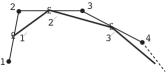
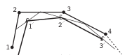
It is easy to see that the process converges to a point - the centroid of the original vertices (and therefore the centroid of the vertices of any polygon in the sequence). Buffon observed a remarkable regularization effect of this procedure: the limiting shape of the polygon is affine regular. Here a polygon is called affine regular if it is affine equivalent to a regular polygon.
In fact such a similar phenomenon was already observed since Roman times. When creating mosaics Roman craftsmen achieved more regular pieces by breaking the corner, so effectively using the same procedure [21]. The explanation is based on simple arguments from linear algebra, see e.g. [1, 29] and next section.
The situation here is different from the theory of the pentagram map, initiated by R. Schwartz in 1990s and extensively studied in recent years, where the dynamics is nonlinear, quasi-periodic and integrable in Arnold-Liouville sense (see [13, 23] and references therein).
In this paper we will study the following natural 3-dimensional version of the Buffon procedure [26]. Let be a simplicial polyhedron in , having all faces triangular. Define its Buffon transformation as the simplicial polyhedron with vertices , where for each vertex of the new vertex is defined as the centroid of the centroids of all edges meeting at The question is what is the limiting shape of as goes to infinity.
Unfortunately, the answer in general is disappointing: the limiting shape will be one-dimensional. Indeed the same arguments from linear algebra show that this shape is determined by the subdominant eigenspace of the corresponding operator on the graph , which is the 1-skeleton of (see the details below), and this eigenspace generically has dimension 1. This means that in order to have a sensible limiting shape we need to add some assumptions on the initial polyhedron
Let be one of the symmetry groups of the Platonic solids: tetrahedron, octahedron/cube, icosahedron/dodecahedron respectively. Assume that the combinatorial structure of the initial polyhedron is -invariant, which means that faithfully acts on the graph
Our main result is the following theorem.
Theorem 1.
Let be a simplicial polyhedron in with -invariant combinatorial structure. Then for a generic the limiting shape obtained by repeatedly applying Buffon procedure to is a star-shaped polyhedron The vertices of are explicitly determined by the subdominant eigenspace of the Buffon operator, which in this case has dimension 3.
The proof is based on the deep results from the spectral theory on graphs due to Colin de Verdière [2] and in particular due to Lovász et al [10, 15, 16], who studied the eigenspace realisations of polyhedral graphs. Both assumptions of the theorem, namely simpliciality and platonic symmetry, are essential.
Recall that the polyhedron is called star-shaped (not to be mixed with star polyhedra like Kepler-Poinsot) if there is a point inside it from which one can see the whole boundary of , or equivalently, the central projection gives a homeomorphism of the boundary of onto a sphere. The precise meaning of the term ”generic” will be clear from the next section.
Let us call polyhedron affine -regular if is affine equivalent to In dimension 2 this is equivalent to affine regularity (see next section). Thus the Buffon procedure produces affine -regular version from a generic polyhedron with the above properties. As far as we know the notion of the affine regularity for polyhedra with non-regular combinatorial structures was not discussed in the literature before.
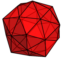
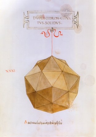
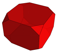
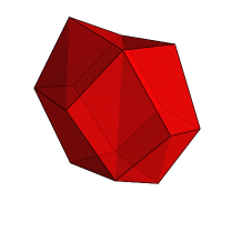
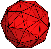
For a generic polyhedron with combinatorial structure of a Platonic solid the corresponding polyhedron is affine regular, which means that it is affine equivalent to the corresponding Platonic solid. For the Archimedean and Catalan solids however, this is no longer true, see the example of pentakis dodecahedron (dodecahedron with pyramids build on its faces) on Fig.2 and in the Appendix.

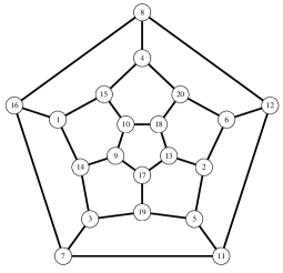
Note that there are plenty of polyhedra with -invariant combinatorial structures, which can be constructed from the Platonic solids using Conway operations [3]. In particular, one will have a simplicial polyhedron by applying to any such the operation, which Conway called and denoted by , consisting of building the pyramids on all the faces. Many examples of the corresponding combinatorial types can be found in chemistry and physics literature in relation with the famous Thomson problem, see e.g. [4].
For non-simplicial polyhedra the Buffon transformation usually breaks the faces, which in general are not recovering even in the limit (see Fig.13 in Appendix B).
The platonic symmetry keeps the limiting shape 3-dimensional, preventing collapse to lower dimension. The dihedral symmetry is not enough: one can check that a polyhedron with prismatic combinatorial structure will collapse to the corresponding affine regular polygon.
The star-shape property of the limiting shape is probably the strongest we can claim since the convexity may not hold as the example of the triakis tetrahedron shows (see Fig. 11 in the Appendix).
The structure of the paper is as follows. In Section 2 we start with the (well-known) solution of the Buffon puzzle for polygons to explain the main ideas and relation to linear algebra. Then, in Section 3, we define the Buffon transformation for polyhedra and review the classical Steinitz theorem which gives graph-theoretical characterisation of 1-skeletons of convex polyhedra. In section 4 we introduce the main tools from spectral graph theory: the Colin de Verdière invariant and null space realisation for polyhedral graphs studied by Lovász et al. In section 5 we use them and representation theory of finite groups to prove our main result. In Appendix A we present the character tables for the polyhedral groups and the corresponding decomposition of the space of functions on the vertices of Platonic solids into irreducible components. In Appendix B we give the spectra of the Buffon operators for some combinatorial types and the corresponding shapes of affine -regular polyhedra.
2. Buffon transformation for polygons.
Consider an arbitrary -gon with vertices described by the column vector
(and an integer ). Generate a second polygon by joining the centres of the consecutive edges of . The corresponding transformation acts on the vertices of as follows:
In matrix form this can be described as
where
After transformations we obtain a polygon with the vertices
Following Buffon we claim that for generic initial polygons the limiting shape of the polygons as increases becomes affine regular. Recall that a polygon is affine regular if it is affine equivalent to a regular polygon.
To prove this we use the following result from Linear Algebra (see e.g. Theorems 5.1.1, 5.1.2 in [28]).
Theorem 2.
(Subspace Iteration Theorem) Let be a real matrix and let be the set of its eigenvalues (in general, complex and with multiplicities) ordered in such a way that
Let and be the dominant and complementary invariant subspaces associated with and respectively and Then for any -dimensional subspace such that the image of under the iterations of
tends to the dominant subspace in the Grassmannian .
To apply this to our case first note that
where the matrix
has the property and the eigenvalues being -th roots of unity. The spectrum of is therefore
The eigenvalues of maximum modulus, other than , are and its complex conjugate .
The dominant subspace in this case corresponds to and is generated by the corresponding eigenvector :
The previous result can be interpreted that as increases converges to a point. To see the limiting shape we should look at the subdominant invariant subspace corresponding to and .
Geometrically one can do this by assuming that the centroid of the vertices is at the origin (centre of mass condition). This means that we restrict the action of on the invariant subspace
This eliminates the eigenvalue and the new dominant subspace corresponding to is precisely the one describing the limiting shape. One can easily check that
Choosing and to be orthogonal unit vectors we see that the corresponding vertices form a regular polygon. In general, the dominant subspace describes all affine regular polygons. The other eigenspaces correspond to the affine regular ”polygrams”.
For example, when we have the eigenvalues
and the corresponding eigenspaces
describing the affine regular pentagons and pentagrams respectively:


3. Buffon transformation for polyhedra
Recall first some basic notions of graph theory and the relation with polyhedra.
A graph consists of a finite set (vertices), together with a subset (edges). We will assume that the graph has no loops and is undirected which means that for each edge we also have .
We say that the vertices and are adjacent and write if there is an edge connecting them. The degree of a vertex is the number of the adjacent vertices.
A graph is connected when there is a path between any two vertices. A graph is called 3-connected if for every pair of vertices and there are at least three paths from to , whose only vertices (or edges) in common are and .
A graph is called planar if an isomorphic copy of the graph can be drawn in a plane, so that the edges which join the vertices only meet (intersect) at vertices.
For every polyhedron one can consider the 1-skeleton , which is the graph formed by the vertices and edges of
One of the oldest results in polytope theory is a remarkable theorem by Ernst Steinitz. It is often referred to as the Steinitz’ fundamental theorem of convex polyhedra and gives a completely combinatorial characterization of the graphs which can be realised as 1-skeletons of 3-dimensional polytopes (see [7, 31]).
Theorem 3.
(Steinitz, 1922) A graph is isomorphic to the 1-skeleton of a 3-dimensional convex polyhedron P if and only if is planar and 3-connected.
The proof given by Steinitz uses a combinatorial reduction technique. A sequence of transformations of into simpler graphs lead to the tetrahedral graph . Reversing the order of these operations one obtains a polyhedral realization of the original graph .
A graph is called regular when every graph vertex has the same degree.
Let be a simplicial polyhedron in with vertices Define the Buffon transformation as a new polyhedron with the vertices being the centroids of all edges, which meet at a vertex [26, 30]:
| (1) |
where is the degree of the vertex
Consider also the linear Buffon operator where is the vector space of functions on the vertices of the graph defined by the same formula:
| (2) |
Remark. One can define the Buffon transformation by taking the centroids of the centroids of all the faces meeting at a vertex [26, 30], but for simplicial polyhedra we have a simple relation for the corresponding operators
which means that the result of the Buffon procedure on faces will be the same as the one on edges.
The matrix of the Buffon transformation in a natural basis in has the form
| (3) |
where is the adjacency matrix: if is adjacent to and 0 otherwise, the diagonal matrix with the degrees of vertices on the diagonal, and is the matrix of transition probabilities of the Markov chain describing the random walk on graph when is adjacent to and 0 otherwise (see [17]).
Note that unless is a regular graph, matrix is not symmetric. In order to bring it to a symmetric form we introduce the normalized adjacency matrix
| (4) |
with matrix elements if is adjacent to and 0 otherwise. It is easy to see that
so is conjugated to the symmetric matrix
In particular, this means that all the eigenvalues of are real. The maximal eigenvalue is and the corresponding eigenvector is
Now we ask the same question: what is the limiting shape of when goes to infinity ?
By the same arguments using the Subspace Iteration Theorem the answer is given by the subdominant eigenspace of the corresponding Buffon operator In general it is one-dimensional, which means that the limiting shape is one-dimensional. However, if we assume additional symmetry we have a three-dimensional limiting shape. To see this we need some results from spectral graph theory, which we present in the next section.
4. Colin de Verdière invariant and null space representation
In 1990 Yves Colin de Verdière [2] introduced a new spectral graph invariant Roughly speaking, is the maximal multiplicity of the second largest eigenvalue of the matrices with the property for adjacent and for non-adjacent and and arbitrary diagonal elements The precise definition is as follows.
Let be a connected undirected graph with the vertex set . Let denote the set of symmetric matrices associated with satisfying
-
(1)
;
-
(2)
has exactly one (simple) negative eigenvalue.
is said to satisfy the Strong Arnold Property if the relation with a symmetric matrix such that for any adjacent and and for implies that . This property is a restriction, which excludes some degenerate choices of the edge weights and the diagonal entries.
The Colin de Verdière invariant is the largest corank of matrices from the set satisfying the Strong Arnold Property. A matrix with corank is called a Colin de Verdière matrix of .
After the change of sign and shift by a scalar matrix the corank, which is the dimension of the null space of becomes the multiplicity of the second largest eigenvalue of .
Colin de Verdière characterised all the graphs with parameter
A graph is called outerplanar if it can be drawn in the plane without crossings in such a way that all of the vertices belong to the unbounded face of the drawing.
Theorem 4.
(Colin de Verdière, 1990)
-
•
if and only if is a path;
-
•
if and only if is outerplanar;
-
•
if and only if is planar.
The planarity characterization is a remarkable result, which will be important for us. The ”only if” part is relatively simple and follows from Kuratowski’s characterisation of the planar graphs [8]. The original proof of the ”if” part was quite involved. Van der Holst [9] substantially simplified it and showed that for 3-connected planar graphs the Strong Arnold property does not play any role.
Corollary 1.
(Van der Holst, 1995) For any matrix from the corank of can not be larger than 3.
In [15] Lovász found an explicit way of constructing the Colin de Verdière matrix for any 3-connected planar graph using the Steinitz’ realisation of as a 1-skeleton of a convex polyhedron This result will be crucial for us, so we will sketch here the main steps of his construction following [15].
Recall first the notion of polarity for polyhedra in , see e.g. [31]. Let be any convex polytope in , containing the origin in its interior. The polar polyhedron is defined as
where denote the scalar product in It is known that is also a convex polyhedron and the 1-skeleton of is the planar dual graph with vertices corresponding to the faces of and edges corresponding to edges of [31].
Now let be Steinitz’ realisation of graph so that is isomorphic to 1-skeleton We can always assume that contains the origin inside it. Consider its polar polyhedron
Let and be two adjacent vertices of , and and be the endpoints of the corresponding edge of . Then by the definition of polarity we have
This implies that is perpendicular to , and similarly to Hence the vectors and the cross-product are parallel and we can find the coefficients such that
We can always choose the labelling of and in such a way that .
This defines for adjacent For non-adjacent and we define to be zero. To define consider the vector
Then
where the last sum is taken over all edges of the face of corresponding to , oriented counterclockwise. Since this sum is zero we have
which means that and are parallel. Therefore we can define by the relation
Theorem 5.
(Lovász, 2000) The matrix described above is a Colin de Verdière matrix for the graph .
Indeed by construction has the right pattern of zeros and negative elements. The condition can be written in the following form
This means that each coordinate of the defines a vector in the kernel of and hence has corank at least 3. But by Corollary 1 it can not be larger than 3, so the corank is 3 and thus maximal.
To prove that has exactly one negative eigenvalue one can use the classical Perron-Frobenius theorem, see e.g. [6].
Theorem 6.
(Perron-Frobenius, 1912) If a real matrix has non-negative entries then it has a nonnegative real eigenvalue which has maximum absolute value among all eigenvalues. This eigenvalue has a real eigenvector with non-negative coordinates. If the matrix is irreducible, then has multiplicity 1 and the corresponding eigenvector can be chosen to be positive.
Choosing sufficiently large we have the matrix which has non-negative entries and irreducible, so we can apply the Perron-Frobenius Theorem to conclude that the smallest eigenvalue of has multiplicity 1. It must be negative since we know that the eigenvalue has multiplicity at least 3. The fact that there are no more negative multiplicities requires a considerable work using the connectivity of the space of Steinitz’ realisations, see [15].
Conversely, having a Colin de Verdière matrix one can consider the following null space representation (see [16]).
Choose a basis in the kernel of and consider a matrix with rows being the coordinates of Then the columns of this matrix give the set of 3-vectors, defining the map The problem is that in general they will not be vertices of a convex polyhedron, but Lovasz [15] showed that after some scaling this is the case (such a scaling he called proper). At the level of the Colin de Verdière matrices this corresponds to the change , where is a non-degenerate diagonal matrix, which obviously preserves the properties of
Theorem 7.
(Lovász, 2000) For a 3-connected planar graph any Colin de Verdière matrix can be properly scaled, so that null space representation gives a convex polyhedron with 1-skeleton isomorphic to .
Note that the change of basis in the kernel of corresponds to a linear transformation of , so the corresponding polyhedron is defined only modulo affine transformation.
Now we are ready to prove our main result.
5. Proof of the main theorem
Let be a Platonic group and a -invariant planar 3-connected graph.
We know after Steinitz that can be realized by a 3-dimensional convex polyhedron , but in the presence of symmetry Mani [18] showed that there is a symmetric realisation
Theorem 8.
(Mani, 1971) There exists a convex polyhedron with the group of isometries isomorphic to and with 1-skeleton isomorphic to
Since is planar and 3-connected, its Colin de Verdière invariant must be 3. Let be the Colin de Verdière matrix given by Lovász construction applied to Mani’s version of Steinitz realisation
Let be the normalised adjacency matrix (4). We know that the matrix of the Buffon transformation is related to by
and that its largest eigenvalue is Let be the second largest eigenvalue of We would like to show that it has multiplicity 3.
To do this consider the symmetric matrix
It is easy to see that and that the corank of is precisely the multiplicity of
Define a parameter family of matrices
| (5) |
where is the Colin de Verdière matrix defined above.
Since is -invariant, the group acts on the kernel of . When we know that the kernel of has dimension 3 and by Lovász result [15] the corresponding representation of is standard geometric by the isometries of
Since this representation is irreducible and the set of 3-dimensional representations of is discrete, by continuity arguments the kernel will remain 3-dimensional geometric representation for all , in particular for .
These arguments will not work only if collides with another eigenvalue. But this could not happen with the negative eigenvalue because of the Perron-Frobenius theorem. In particular, all matrices belong to If this happens with a positive eigenvalue we will have the corank of the corresponding to be at least 4, which contradicts to the Colin de Verdière result.
Thus we have proved that the kernel of is 3-dimensional, and hence the same is true for the subdominant eigenspace of the Buffon operator The limiting shape is given essentially by the null space representation construction, but the proper scaling may not hold. However, the very existence of a proper scaling [15, 16] and the assumption of simplicity imply that the corresponding vectors are the vertices of a certain star-shaped polyhedron with 1-skeleton isomorphic to The triakis tetrahedron example below shows that the proper scaling is indeed not automatic, so the convexity property does not necessary hold.
This completes the proof of Theorem 1.
6. Concluding remarks.
The Buffon regularisation procedure can be interpreted as search of an ideal shape of a given polyhedron and in that sense can be considered as one of the earliest examples of the trend, popular in modern differential geometry.
For manifolds this usually leads to the solutions of certain nonlinear PDEs like the mean curvature flow in the theory of minimal surfaces [11] or the celebrated Ricci flow in Thurston’s geometrization programme [20]. Our case is conceptually closer to the description of the minimal submanifolds in the unit sphere using the eigenfunctions of the Laplace-Beltrami operator, see [14, 25].
The main difference with the differential case is that the generic graphs are much less regular objects than manifolds, even under our assumption of Platonic symmetry. The crucial thing here is a large multiplicity of the second eigenvalue of the Buffon operator. How to guarantee this is a good question.
The symmetry assumption seems to be natural. In this relation we would like to mention an interesting result of Mowshowitz [22], who showed that if all eigenvalues of the adjacency matrix of a graph are different, then every automorphism of has order 1 or 2. Some interesting related results for the graphs with vertex transitive group action can be found in [12]. Note that in our case the group action is far from being vertex transitive.
An interesting question concerns the decomposition of into the irreducible -modules with respect to the Buffon spectrum. We saw that the geometric representation always appears at the subdominant level, but we do not know much about higher level. For the regular polyhedra the answer is given in Appendix A.
It would be interesting to understand what our geometric analysis means for related random walk on the corresponding graphs.
Finally, a natural question is what happens in higher dimension. We believe that for the simplicial polyhedra we should expect similar result if we assume the symmetry under an irreducible Coxeter group. Note that in dimension 4 we have 6 regular polyhedra with the symmetry groups , , and while in dimension more than 4 we have only analogues of tetrahedron, cube and octahedron.
7. Acknowledgements.
We are grateful to Jenya Ferapontov, Steven Kenny, Boris Khesin and László Lovász for very helpful discussions. Special thanks are to Graham Kemp, who was part of these discussions for quite a while.
References
- [1] E.R. Berlekamp, E.N. Gilbert and F.W. Sinden A Polygon Problem. The American Mathematical Monthly, Mathematical Association of America, 72 (1965), 233–241.
- [2] Y. Colin de Verdière Sur un nouvel invariant des graphes et un critère de planarité. J. Combin. Theory Ser. B 50 (1990), 11–21. English translation: On a new graph invariant and a criterion for planarity. In Graph Structure Theory (N. Robertson, P. Seymour, Eds.), Contemporary Mathematics, pp. 137–147, AMS, Providence, RI, 1993.
- [3] J.H. Conway, H. Burgiel, C. Goodman-Strass The Symmetries of Things. A.K. Peters, Ltd, 2008.
- [4] J. R. Edmundson The arrangement of point charges with tetrahedral and octahedral symmetry on the surface of a sphere with minimum Coulombic potential energy. Acta Cryst. (1993). A49, 648-654.
- [5] Fulton W., Harris J. Representation Theory. Springer, 1991.
- [6] F. Gantmacher The Theory of Matrices. Chelsea, NY, 1977.
- [7] B. Grunbaum Graphs of polyhedra; polyhedra as graphs. Discrete Mathematics, 307 (2007), 445-463.
- [8] F. Harari Graph Theory. Addison Wesley, Reading, MA, 1969.
- [9] H. van der Holst A short proof of the planarity characterization of Colin de Verdière. J. Comb. Theory Ser. B 65 (1995), 269-272.
- [10] H. van der Holst, L. Lovász and A. Schrijver The Colin de Verdière graph parameter. In Graph Theory and Combinatorial Biology, Bolyai Soc. Math. Stud. 7 (1999), 29-85.
- [11] G. Huisken Flow by mean curvature of convex surfaces into spheres. J. Differential Geom. 20 (1984), 237-266.
- [12] I. Ivrissimtzis, N. Peyerimhoff Spectral representations of vertex transitive graphs, Archimedean solids and finite Coxeter groups. Groups Geom. Dyn. 7 (2013), no. 3, 591-615.
- [13] B. Khesin, F. Soloviev Integrability of higher pentagram maps. Math. Ann. 357 (2013), no. 3, 1005 1047.
- [14] S. Kobayashi, K. Nomizu Foundations of differential geometry, Vol. II. John Wiley and Sons, Inc., New York-London- Sydney, 1969.
- [15] L. Lovász Steinitz representations of polyhedra and the Colin de Verdière number. J. Comb. Theory, Ser. B, 82 (2000), 223–236.
- [16] L. Lovász and A. Schrijver On the null space of a Colin de Verdière matrix. Symposium la Mémoire de Francois Jaeger (Grenoble, 1998). Ann. Inst. Fourier (Grenoble) 49 (1999), no. 3, 1017–1026.
- [17] L. Lovász Random Walks on Graphs: A Survey. Bolyai Soc. Math. Stud, 2. Combinatorics, Paul Erdös is Eighty (Volume 2) Keszthely (Hungary), 1993, 1-46.
- [18] P. Mani Automorphismen von polyedrischen Graphen. Mathematische Annalen, 192 (1971), 279–303.
- [19] B. McConnell Spectral realizations of graphs. http://daylateanddollarshort.com/mathdocs/Spectral-Realizations-of-Graphs.pdf
- [20] J. Morgan and G. Tian Ricci flow and the Poincare conjecture. Clay Mathematics Monographs, Vol. 3, 2007.
- [21] MOSAIC 11, Journal of Asprom, 1984.
- [22] A. Mowshowitz The group of a graph whose adjacency matrix has all distinct eigenvalues. In ”Proof Techniques in Graph Theory” pp. 109-110, Academic Press, New York, 1969.
- [23] V. Ovsienko, R.E. Schwartz, S. Tabachnikov Liouville-Arnold integrability of the pentagram map on closed polygons. Duke Math. J. 162 (2013), no. 12, 2149-2196.
- [24] Saldanha N.C., Tomei C. Spectra of regular polytopes. Discrete Comput. Geom. 7(4) (1992), 403-414.
- [25] T. Takahashi Minimal immersions of Riemannian manifolds. J. Math. Soc. Japan 18:4 (1966), 380-385.
- [26] A.P. Veselov and J.P. Ward, unpublished (2004).
- [27] D. Wells You are a Mathematician. London Penguin Books, 1995
- [28] D. S. Watkins The Matrix Eigenvalue Problem: GR and Krylov Subspace Methods. SIAM, 2007.
- [29] J.P. Ward Experimental mathematics in the curriculum (part I). Teaching Mathematics Applications. 25 (4)(2006): 205-215.
- [30] J.P. Ward Experimental mathematics in the curriculum (part II). Teaching Mathematics Applications. 26 (1)(2007): 27-37.
- [31] G. Ziegler Lectures on Polyhedra. Springer, 2007.
Appendix A. The symmetry groups of Platonic solids and their characters
The symmetry group of a regular tetrahedron is and is isomorphic to the permutation group of the vertices.
The full symmetry group of the octahedron is the same as for the cube: . is the rotation subgroup, which is isomorphic to the permutation group of the 4 long diagonals, and corresponds to the central symmetry of cube.
For the icosahedron and dodecahedron the full symmetry group is known to be where is the alternating subgroup of describing the rotational symmetry and is again the central symmetry of the solids.
The irreducible representations of the group have the the form , where and are irreducible representations of and respectively. Note that is either trivial or sign representation of which we will denote respectively by 1 and . Thus we need only the character tables of the groups and , which in the notations of Fulton and Harris [5] are given below in Tables 1 and 2.
| 24 | 1 | 6 | 8 | 6 | 3 |
|---|---|---|---|---|---|
| 1 | (12) | (123) | (1234) | (12)(34) | |
| 1 | 1 | 1 | 1 | 1 | |
| 1 | -1 | 1 | -1 | 1 | |
| 3 | 1 | 0 | -1 | -1 | |
| 3 | -1 | 0 | 1 | -1 | |
| 2 | 0 | -1 | 0 | 2 |
| 60 | 1 | 20 | 15 | 12 | 12 |
|---|---|---|---|---|---|
| 1 | (123) | (12)(34) | (12345) | (21345) | |
| 1 | 1 | 1 | 1 | 1 | |
| 4 | 1 | 0 | -1 | -1 | |
| 5 | -1 | 1 | 0 | 0 | |
| 3 | 0 | -1 | |||
| 3 | 0 | -1 |
With these notations the geometric representations are: for tetrahedral group for cube/octahedral group and for icosahedral/dodecahedral group
The corresponding decompositions of the space of functions on the vertices into irreducible -modules are
| (6) |
for tetrahedron,
| (7) |
for octahedron,
| (8) |
for cube,
| (9) |
for icosahedron,
| (10) |
for dodecahedron.
We have ordered them according to the appearance in the spectrum of the Buffon operator. It turns out that in all these cases the spectral decomposition coincides with -decomposition (see the examples below). Note that the first two are always trivial and geometric representations in agreement with our result.
Appendix B. Examples of Buffon realizations of polyhedra
For the polyhedra with combinatorial structure of Platonic solids the Buffon procedure leads to the polyhedron , which is affine equivalent to the regular realisation of
Since in the regular case the Buffon matrix can be replaced by the adjacency matrix the calculations are essentially the same as in [19], where one can find a lot more experimental data. The calculation of spectra of regular polytopes can be found in [24].
We present here the most instructive examples of Buffon realisations of regular, Archimedean and Catalan solids. All the calculations and pictures were made using Mathematica.
Recall that the Archimedean solids (also referred to as the semi-regular polyhedra) are the convex polyhedra with faces being regular polygons of two or more different types arranged in the same way about each vertex. Solids with a dihedral group of symmetries (e.g., regular prisms and antiprisms) are not considered to be Archimedean solids. With this restriction there are 13 Archimedean solids. For Archimedean solids the affine -regular version is in general is not affine equivalent to the standard one (see below the example of truncated cube).
The Catalan solids are duals of the Archimedean solids. The Catalan solids are convex polyhedra with regular vertex figures (of different types) and with equal dihedral angles. For Catalan solids the affine -regular versions may not be convex or, in non-simplicial case, may even not exist (see the examples below).
We start with the regular cases of icosahedron and dodecahedron to show the relation with -decomposition and to look at the embeddings related to other eigenvalues.
The Icosahedron
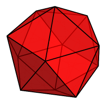
The eigenspaces corresponding to the second highest eigenvalue and its conjugate eigenvalue are:
where and .
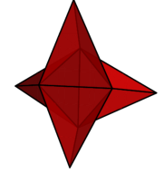
Geometrically, describes an affine regular icosahedron, while corresponds to an affine great icosahedron, which is one of four Kepler-Poinsot regular star polyhedra.
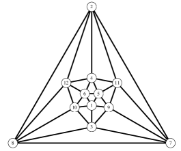
The eigenspace describes the 5-dimensional realisation of an icosahedron as a 5-simplex: 6 pairs of opposite vertices identified with 6 vertices of the simplex.
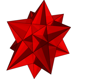
The Dodecahedron
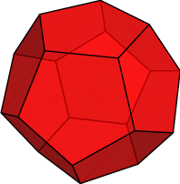
The eigenspaces corresponding to the second highest eigenvalue and to its conjugate are:
where and .
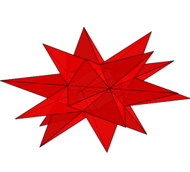
Geometrically, describes an affine regular dodecahedron, while corresponds to an affine version of the great stellated dodecahedron, which is another Kepler-Poinsot polyhedron (see Fig. 7).
It is a bit puzzling that the remaining two Kepler-Poinsot polyhedra (small stellated dodecahedron and great dodecahedron) seem to not appear in Buffon approach.
The 3 remaining eigenspaces are:
corresponds to the 5-dimensional embedding of dodecahedron with ”broken faces”. It would be interesting to understand the geometry of the -dimensional embeddings corresponding to and Since in the second case the opposite vertices identified it corresponds to the representation in agreement with (10).
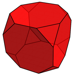
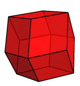
The Truncated Cube
is one of the Archimedean solids, for which Buffon realisation is not affine equivalent to the standard one.
The corresponding Buffon spectrum is:
The eigenspace corresponding to the second highest eigenvalue is:
The facing octagons of the geometric realisation of are not affine regular: one can check that while for the regular octagon Thus the affine -regular truncated cube obtained by the Buffon procedure is not an affine version of the regular truncated cube.
Triakis Tetrahedron
is the Catalan solids dual to the truncated tetrahedron. This is the simplest case when convexity does not hold for Buffon realisation.
![[Uncaptioned image]](/html/1402.5354/assets/x15.png)
![[Uncaptioned image]](/html/1402.5354/assets/x16.png)
The corresponding Buffon eigenvalues are:
The eigenspaces corresponding to the eigenvalues and to are:
A particular geometric realisation derived from is shown in Figure 12:
As shows the vertices coalesce together pairwise. The corresponding geometrical realisation gives a general tetrahedron.
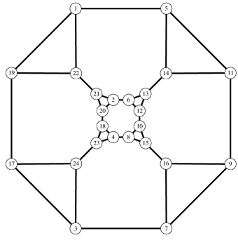
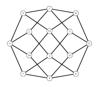
The Rhombic Dodecahedron
is the Catalan solid dual to cuboctahedron. We will see that it does not admit Buffon realisation.
The corresponding eigenvalues are:
The -dimensional eigenspaces corresponding to the eigenvalues and are:
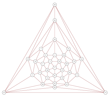
Both eigenspaces and fail to correspond to a polyhedron with the combinatorial structure of the -skeleton of the rhombic dodecahedron. A particular graph realisation obtained from the eigenspace is shown in Fig. 13.
Pentakis Dodecahedron
is the Catalan solid dual to the truncated icosahedron, which we mentioned in the Introduction.
The corresponding Buffon eigenvalues are:
The subdominant eigenspace corresponds to:
where
The corresponding Buffon realization is shown below. It is convex and looks pretty similar to the Catalan version, but the pyramids are slightly higher. The ratios of the height of a pyramid to the distance of its top vertex from the centre in the Catalan and Buffon cases are and respectively.
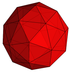
The self-intersecting realisations corresponding to other multiplicity 3 eigenvalues are shown below.
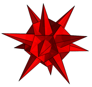
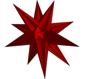
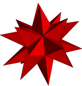
To finish we present Mathematica image of the cumulated dodecahedron with all edges of equal length, featured on Leonardo’s drawing (Fig.2):