Approximation of Riemann’s zeta function by finite Dirichlet series: multiprecision numerical approach

Abstract

The finite Dirichlet series from the title are defined by the condition that they vanish at as many initial zeroes of the zeta function as possible. It turned out that such series can produce extremely good approximations to the values of Riemann’s zeta function inside the critical strip. In addition, the coefficients of these series have remarkable number-theoretical properties discovered in large scale high accuracy numerical experiments.

So far no theoretical explanation to the observed phenomena was found.

1 Introduction

One of the most important open problems in Number Theory is the famous Riemann Hypothesis stated in [Riemann 1859]. At the turn of the century, it was included by David Hilbert as part of his 8th problem, one among 23 most important, in his opinion, problems [Hilbert 1900] left open for the coming 20th century. The Riemann Hypothesis resisted all numerous attempts to (dis)proof it and was recognized by the Clay Institute as one of the 7 Millennium problems [Clay].

The Riemann Hypothesis, RH for short, is a statement about complex zeroes of Riemann’s zeta function. This function can be defined via Dirichlet series

$$\zeta(s)=\sum_{n=1}^{\infty}n^{-s}.$$ (1)

This series converges only for ${\mathrm{Re}}(s)>1$ but the function can be analytically continued to the whole complex plane with the exception of the point $s=1$ which is its only pole.

The zeta function for real $s$ was studied already by Leonhard Euler. In particular, he gave in [Euler 1737] another definition of the function via a product, namely,

$$\sum_{n=1}^{\infty}\frac{1}{n^{s}} = \prod_{p\ \mathrm{prime}}\left(1+\frac{1}{{p^{s}}}+\frac{1}{{p^{2s}}}+\dots\right).$$ (2)

This equality can be viewed as an analytic form of the Fundamental Theorem of Arithmetic stating that every natural number has a unique factorization into the product of powers of primes—just expand the right hand side in (2) and get its left hand side.

The fact that Euler product, the right hand side of (2), is taken over prime numbers, explains the role played by the zeta function in the study of these numbers. In particular, Euler proved anew the infinitude of prime numbers, and the beauty of his proof can rival that of the original proof given by Euclid: if the number of primes were finite, then for $s=1$ the divergent harmonic series, that is, the left hand side of (2), would have finite value equal to the right hand side of (2).

Bernhard Riemann went further, he showed that the zeta function can be used for the study of the growth of the prime counting function $\pi(x)$ equal to the number of primes not exceeding $x$. This is a step function having a jump of size $1$ at each prime number.

In a more transparent way the relationship between the zeroes of the zeta function and distribution of prime numbers can be be expressed in terms of another step function, $\psi(x)$, defined by Pafnutij Chebyshev in [Chebyshev 1852] as

$$\psi(x) = \ln(\mathrm{LCM}(1,2,...,\lfloor x\rfloor)).$$ (3)

Similar to $\pi(x)$, this function also has a jump at each prime $p$ but now of increasing size $\ln(p)$, and besides it has a jump of the same size at every power of $p$ as well. Hans Carl Friedrich von Mangoldt [Mangoldt 1895] proved that for non-integer $x$ greater than $1$

$$\psi(x) = x-\sum_{\zeta(\rho)=0}\frac{x^{\rho}}{\rho}-\ln(2\pi).$$ (4)

According to (4), the growth of the difference $\psi(x)-x$ depends on the real parts of the zeros of the zeta function. Already Euler knew that this function vanishes at negative even integers, and they are nowadays called the trivial zeroes. Riemann proved that they are the only real zeroes of the zeta function and that all other, non-trivial zeroes lie inside the so-called critical strip $0\leq{\mathrm{Re}}(s)\leq 1$.

Riemann’s Hypothesis predicts that in fact the non-trivial zeros lie on the critical line ${\mathrm{Re}}(s)=\frac{1}{2}$. In terms of Chebyshev’s function RH can be restated as

$$\psi(x)=x+O(x^{\frac{1}{2}}\ln^{2}(x))$$ (5)

and in terms of the function $\pi(x)$ as

$$\pi(x)=\int^{x}\frac{{\mathrm{d}}t}{\ln(t)}+O(x^{\frac{1}{2}}\ln(x)).$$ (6)

Many researchers verified the validity of RH for initial zeroes of the zeta function via finite computations giving, nevertheless mathematically rigourously, the exact value $\frac{1}{2}$ for their real parts. The last achievement reported in [Gourdon 2004] tells that this is so for impressive $10^{13}$ initial (pairs of conjugate) zeroes of the zeta function.

Numerical studies of the zeta function are valuable from the perspective of discovering interesting patterns in its behaviour, providing preliminary evidence for undiscovered phenomena, and formulating hypotheses that are not obvious from the analytic formulas. In this article we followed such an approach, by studying numerically various quantities related to approximation the zeta function by finite Dirichlet series.

The simplest form of such series is just the truncation

$$\zeta_{N}(s)=\sum_{n=1}^{N}n^{-s}.$$ (7)

Paul Turán [Turan 1948] established that for proving the Riemann Hypothesis it would be sufficient to show that

$$\sup\{{\mathrm{Re}}(s):\zeta_{N}(s)=0\}=1+O(N^{-\frac{1}{2}}).$$ (8)

However, Hugh Lowell Montgomery [Montgomery 1983] proved that in fact

$$\sup\{{\mathrm{Re}}(s):\zeta_{N}(s)=0\}=1+\Omega_{+}\!\!\left({\frac{\ln\ln(N)}{\ln(N)}}\right),$$ (9)

which implies that (8) does not hold, and hence one cannot prove RH in that way.

Partial sums of Riemann’s zeta-function were also studied by Michel Balazard and Oswaldo Velásquez Castañón in [Balazard et al 2009], by Peter Borwein, Greg Fee, Ron Ferguson, and Alexa Van Der Waall in [Borwein et al 2007], by Steven M. Gonek and Andrew H. Ledoan in [GonekLedoan 2010], by Norman Levinson in [Levinson 1973], by Robert Spira in [Spira 1966, Spira 1968, Spira 1972], and by Sergej Voronin in [Voronin 1974].

In this article we report on numerical studies of coefficients of finite Dirichlet series that are constructed not by truncating the infinite series (1) but on the basis of a few initial non-trivial zeroes of the zeta function. Firstly, we found that such finite Dirichlet series approximate well many of the subsequent non-trivial zeroes and a number of initial trivial zeroes. This finding (originally observed for a slightly different approximation in [Matiyasevich 2012]) was quite unexpected.

Secondly, numerical experiments with very high accuracy revealed that these coefficients have very rich fine structure related to prime numbers.

The article is structured as follows. In Section 2 we introduce our objects of study. Section 3 describes the initial findings. Section 4 is devoted to technical details of performing the calculations. In Sections 5–6 we discussed numerically observed phenomena. In Section 7 we briefly present some similar experiments and our plans for new calculations. In Section 8 we summarize our discoveries.

2 Our objects for examination

We are to approximate the zeta function by finite Dirichlet series having the form

$$\Delta_{N}(s)=\sum_{n=1}^{N}\delta_{N,n}n^{-s}$$ (10)

with some weight coefficients $\delta_{N,n}$. These coefficients will be selected in such a way that the finite series (10) and (the function defined by) infinite series (1) would have $N-1$ common zeroes.

The non-trivial zeroes come in conjugate pairs:

$$\dots=\zeta(\overline{\rho_{3}})=\zeta(\overline{\rho_{2}})=\zeta(\overline{\rho_{1}})=0=\zeta(\rho_{1})=\zeta(\rho_{2})=\zeta(\rho_{3})=\dots$$ (11)

Assuming that they are simple and satisfy RH, we write

$$\rho_{n}=\frac{1}{2}+{\mathrm{i}}\gamma_{n}$$ (12)

with

$$\qquad 0<\gamma_{1}<\gamma_{2}<\gamma_{3}\dots$$ (13)

We will always take for $N$ an odd number, $N=2M+1$, put $\delta_{N,1}=1$ and determine the remaining coefficients in (10) by the condition

$$\Delta_{N}\left(\frac{1}{2}\pm{\mathrm{i}}\gamma_{k}\right)=0,\quad k=1,\dots,M.$$ (14)

This condition gives explicit expressions for the coefficients in (10), namely,

$$\delta_{N,n}=\frac{\tilde{\delta}_{N,n}}{\tilde{\delta}_{N,1}},$$ (15)

where

$$\tilde{\delta}_{N,n}=(-1)^{n+1}\times$$ (16)

$$\begin{vmatrix}1&1&\dots&1&1\\ \vdots&\vdots&\ddots&\vdots&\vdots\\ (n-1)^{-\overline{\rho_{1}}}&(n-1)^{-{\rho_{1}}}&\dots&(n-1)^{-\overline{\rho_{M}}}&(n-1)^{-\rho_{M}}\\ (n+1)^{-\overline{\rho_{1}}}&(n+1)^{-{\rho_{1}}}&\dots&(n+1)^{-\overline{\rho_{M}}}&(n+1)^{-\rho_{M}}\\ \vdots&\vdots&\ddots&\vdots&\vdots\\ N^{-\overline{\rho_{1}}}&N^{-\rho_{1}}&\dots&N^{-\overline{\rho_{M}}}&N^{-\rho_{M}}\end{vmatrix}.$$

3 First observations

Our interest was to examine numerical values of the determinants (16). Originally, it was guessed that with the growth of $N$ the coefficients $\delta_{N,n}$ (defined by (15)) will approach the coefficients from (1), that is, for a fixed $n$

$$\delta_{N,n}\underset{N\rightarrow\infty}{\longrightarrow}1.$$ (17)

This guess was based on an expected analogy with the Taylor series. Namely, if

$$1+\sum_{n=1}^{\infty}a_{n}z^{n}=\prod_{k=1}^{\infty}\left(1-\frac{z}{z_{k}}\right)$$ (18)

and

$$1+\sum_{n=1}^{N}a_{N,n}z^{n}=\prod_{k=1}^{N}\left(1-\frac{z}{z_{k}}\right)$$ (19)

then for a fixed $n$

$$a_{N,n}\underset{N\rightarrow\infty}{\longrightarrow}a_{n}.$$ (20)

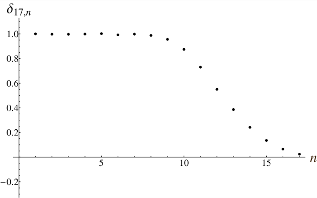
Figure 1: Coefficients $\delta_{17,n}$

Initial calculations seemed to support (17) – see Figure 1. This figure justifies our writing

$$\Delta_{17}(s)=\sum_{n=1}^{17}\delta_{17,n}n^{-s}\leftrightharpoons\sum_{n=1}^{\infty}n^{-s}=\zeta(s)$$ (21)

with the ideograph $\leftrightharpoons$ having here and in the sequel a very weak sense: a few initial coefficients of the two Dirichlet series are approximately equal.

It turned out that $\Delta_{17}(s)$ gives a rather good approximation to $\zeta(s)$ on the critical line, see Figures 2–3.

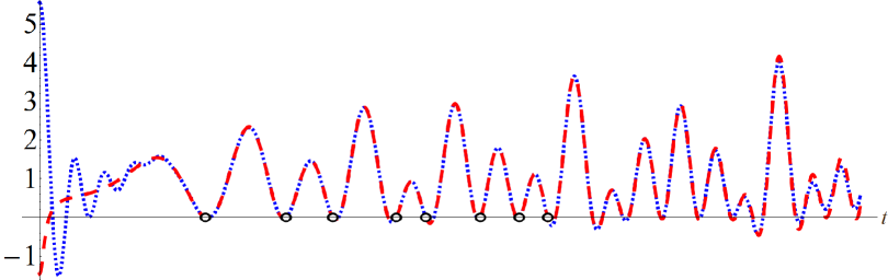
Figure 2: Real parts of $\zeta(\frac{1}{2}+{\mathrm{i}}t)$ (dashed) and $\Delta_{17}(\frac{1}{2}+{\mathrm{i}}t)$ (dotted).

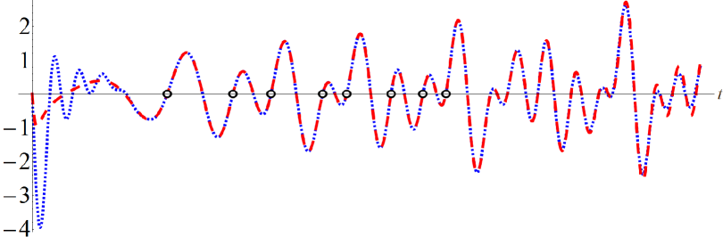
Figure 3: Imaginary parts of $\zeta(\frac{1}{2}+{\mathrm{i}}t)$ (dashed) and $\Delta_{17}(\frac{1}{2}+{\mathrm{i}}t)$ (dotted).

Table 1: Zeroes of $\Delta_{17}(s)$ nearby zeros of $\zeta(s)$

0	=	$\Delta_{17}(\rho_{9}-4.396\dotsc\cdot 10^{-3}+5.711\dotsc\cdot 10^{-3}{\mathrm{i}})$
0	=	$\Delta_{17}(\rho_{10}-1.141\dotsc\cdot 10^{-2}-3.345\dotsc\cdot 10^{-3}{\mathrm{i}})$
0	=	$\Delta_{17}(\rho_{11}-1.498\dotsc\cdot 10^{-2}+1.762\dotsc\cdot 10^{-3}{\mathrm{i}})$
0	=	$\Delta_{17}(\rho_{12}-1.158\dotsc\cdot 10^{-2}+2.264\dotsc\cdot 10^{-2}{\mathrm{i}})$
0	=	$\Delta_{17}(\rho_{13}-1.317\dotsc\cdot 10^{-2}+7.545\dotsc\cdot 10^{-2}{\mathrm{i}})$
0	=	$\Delta_{17}(\rho_{14}-7.400\dotsc\cdot 10^{-2}-5.559\dotsc\cdot 10^{-4}{\mathrm{i}})$
0	=	$\Delta_{17}(\rho_{15}+4.486\dotsc\cdot 10^{-2}+8.379\dotsc\cdot 10^{-2}{\mathrm{i}})$

In particular, $\Delta_{17}(s)$ has zeroes close to a few zeta zeroes following zeroes $\rho_{1}$, …$\rho_{8}$ used for constructing this finite Dirichlet series, see Table 1. Nothing similar can happen for Taylor series – clearly, the finite product in (19) contains no information about the subsequent zeroes $z_{N+1}$, $z_{N+2}$, …

The closeness of the values of $\Delta_{17}(s)$ and its zeroes to the values of $\zeta(s)$ and its zeroes is surprising for two reasons:

• the meaning of the relation $\leftrightharpoons$ in (21) is very week;

• the infinite series in (21) diverges on the critical line.

4 Numerical strategies and pitfalls

The initial observations prompted more thorough numerical studies of the determinants (16) in order to understand better their behaviour for larger $N$. While experimental numerical values can certainly point to some interesting patterns, inaccurate experimental results can become false leads, that are due solely to numerical artifacts. For this reason we aimed at providing numerical evidence at a very high precision level, ideally with tight error bounds, as to minimise the likelihood of false leads.

We were aware that calculation of the determinants (16) could lead to losses of accuracy, and decided to perform calculations with very high precision of over ten thousand decimal places. Such an accuracy was achieved by using multiprecision arithmetic, implemented in such packages as GMP [GMP], Arprec [Bailey 2013] and Arb [Johansson 2013]. This accuracy allowed us to separate numerical artifacts due to the loss of precision in numerical calculations from some interesting phenomena reported in the subsequent sections.

Let us describe our computational settings. The values $\delta_{N,n}$ were computed from $\gamma_{1},\ldots,\gamma_{M}$ by calculating a sequence of determinants ($N=1,2,3,\ldots,12000$) of a matrix with entries $a_{ij}=i^{-\rho_{k}}$ for even $j=2k$ and $a_{ij}=i^{-\bar{\rho}_{k}}$ for odd $j=2k-1$. The determinants were computed by using a variant of Gauss elimination as reported in [BeliakovMatiyasevich 2013], in multiprecision arithmetics, using ten thousand decimal places accuracy. The values of $\gamma_{k}$ were precomputed with twenty thousand decimal places by the authors using Newton-based root finding routine by Fredrik Johansson in his new system Arb [Johansson 2013].

These values are available at [MatiyasevichBeliakov 2013] and more accurate values are at [BeliakovMatiyasevich 2013a]. The library GMP [GMP] was used for multiprecision arithmetics, and computations were performed in parallel on an MPI-based cluster involving 168 processes and 400 GB combined RAM, thanks to VPAC and Monash e-research centre http://www.vpac.org and http://www.monash.edu.au/eresearch/.

The loss of accuracy in Gauss elimination was estimated by computing the same quantities with 20000 decimal places (but for smaller $N$ up to $6000$, due to limitations on computer resources available at the time). Thus we had an estimate for the accuracy of the computed coefficients $\delta_{N,n}$. This estimate suggested that the chosen accuracy of 10000 decimal places was in fact warranted due to cancelation errors, and that it was also sufficient for numerical studies up to $N=12001$.

However, this accuracy turns out to be insufficient when we are to examine subtler structure of the coefficients presented in Section 6 – cf. Figure 7 with Figure 9, the lower dots on the latter lie on a horizontal line only because of the lost of accuracy.

Of course, given the computational cost of Gauss elimination and of multiprecision arithmetics, a sufficiently large cluster of processors and combined RAM were needed. The details of our computations are presented in [BeliakovMatiyasevich 2013]. Briefly, we were able to compute the sequence of determinants $\delta_{N,n},n=1,\ldots,N,N=1,2,\ldots,\bar{N}$ in just one Gauss elimination in $O(\bar{N}^{3})$ time and using $\bar{N}^{2}+O(\bar{N})$ storage. In our computations we took $\bar{N}=12001$. All computations were parallelised with particular attention to load balancing, and computations took seven days on a cluster with 168 processes (Intel E5-2670 nodes with $48-64$ GB of RAM, connected by 4x QDR Infiniband Interconnect, running CentOS 6 Linux).

5 Discoveries for larger $N$

The multiprecision calculations for large $N$ up to 12001 produced interesting findings. Firstly, we found that for large $N$ the series $\Delta_{N}$ (10) continues to provide very accurate approximations to the zeros of the zeta function but doesn’t approximate its value at other points any longer; these phenomena will be discussed in this Section. Secondly, high accuracy experiments allowed us to look ‘‘under a microscope’’ at the fine structure of the coefficients $\delta_{N,n}$. Coefficients which unsuspiciously looked as alternating values $+1$ and $-1$ have shown very rich fine structure at the precision level between $10^{-1000}$ and $10^{-10000}$, the structure that unexpectedly revealed prime numbers! The patterns revealed are so remarkable and regular that we are convinced they could not be due to numerical artifacts. We detail these observations in the next Section.

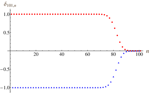
Figure 4: Coefficients $\delta_{101,n}$ (disks for even $n$ and triangles for odd $n$)

High accuracy calculations for larger $N$ revealed that most likely the guess (17) was wrong, and this explains why the values of $\Delta_{N}(s)$ aren’t close to $\zeta(s)$ any longer. Figure 4 exhibits coefficients $\delta_{101,n}$. Such behaviour is ‘‘typical’’ for $N>100$, however, every now and then a kind of ‘‘Gibbs phenomenon’’ occurred as illustrated on Figure 5, or even more bizarre behaviour as on Figure 6; presumably, such irregularities would disappear for $N$ big enough.

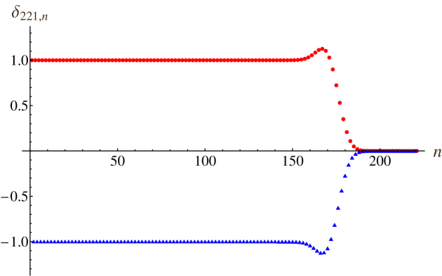
Figure 5: Coefficients $\delta_{221,n}$ (disks for even $n$ and triangles for odd $n$)

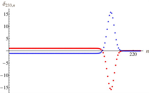
Figure 6: Coefficients $\delta_{233,n}$ (disks for even $n$ and triangles for odd $n$)

A catalog of $\delta_{N,n}$ for many values of $N$ can be found in [Matiyasevich]. Its content suggests that (17) should be replaced by

$$\delta_{N,n}\underset{N\rightarrow\infty}{\longrightarrow}(-1)^{n+1}$$ (22)

and, respectively, for large $N$

$$\Delta_{N}(s)=\sum_{n=1}^{N}\delta_{N,n}n^{-s}\leftrightharpoons\sum_{n=1}^{\infty}(-1)^{n+1}n^{-s}=\eta(s)$$ (23)

where

$$\eta(s)=(1-2\cdot 2^{-s})\zeta(s)$$ (24)

is the alternating zeta function.

Table 2: Zeroes of $\Delta_{3001}(s)$ nearby zeroes of $1-2\cdot 2^{-s}$

0	=	$\Delta_{3001}(1+\frac{2\pi{\mathrm{i}}}{\ln(2)}\cdot 50-1.032\dotsc\cdot 10^{-127}+1.020\dotsc\cdot 10^{-127}{\mathrm{i}})$
0	=	$\Delta_{3001}(1+\frac{2\pi{\mathrm{i}}}{\ln(2)}\cdot 100-2.433\dotsc\cdot 10^{-129}+2.065\dotsc\cdot 10^{-127}{\mathrm{i}})$
0	=	$\Delta_{3001}(1+\frac{2\pi{\mathrm{i}}}{\ln(2)}\cdot 150+1.032\dotsc\cdot 10^{-127}+1.069\dotsc\cdot 10^{-127}{\mathrm{i}})$
0	=	$\Delta_{3001}(1+\frac{2\pi{\mathrm{i}}}{\ln(2)}\cdot 200+4.865\dotsc\cdot 10^{-129}+1.146\dotsc\cdot 10^{-130}{\mathrm{i}})$
0	=	$\Delta_{3001}(1+\frac{2\pi{\mathrm{i}}}{\ln(2)}\cdot 250-1.031\dotsc\cdot 10^{-127}+9.721\dotsc\cdot 10^{-128}{\mathrm{i}})$
0	=	$\Delta_{3001}(1+\frac{2\pi{\mathrm{i}}}{\ln(2)}\cdot 300-7.294\dotsc\cdot 10^{-129}+2.063\dotsc\cdot 10^{-127}{\mathrm{i}})$
0	=	$\Delta_{3001}(1+\frac{2\pi{\mathrm{i}}}{\ln(2)}\cdot 350+1.029\dotsc\cdot 10^{-127}+1.117\dotsc\cdot 10^{-127}{\mathrm{i}})$
0	=	$\Delta_{3001}(1+\frac{2\pi{\mathrm{i}}}{\ln(2)}\cdot 400+9.720\dotsc\cdot 10^{-129}+4.583\dotsc\cdot 10^{-130}{\mathrm{i}})$
0	=	$\Delta_{3001}(1+\frac{2\pi{\mathrm{i}}}{\ln(2)}\cdot 450-1.027\dotsc\cdot 10^{-127}+9.235\dotsc\cdot 10^{-128}{\mathrm{i}})$
0	=	$\Delta_{3001}(1+\frac{2\pi{\mathrm{i}}}{\ln(2)}\cdot 500-1.217\dotsc\cdot 10^{-110}+3.892\dotsc\cdot 10^{-111}{\mathrm{i}})$
0	=	$\Delta_{3001}(1+\frac{2\pi{\mathrm{i}}}{\ln(2)}\cdot 550-1.260\dotsc\cdot 10^{-66}+1.455\dotsc\cdot 10^{-67}{\mathrm{i}})$
0	=	$\Delta_{3001}(1+\frac{2\pi{\mathrm{i}}}{\ln(2)}\cdot 600-2.580\dotsc\cdot 10^{-36}+2.947\dotsc\cdot 10^{-36}{\mathrm{i}})$

Table 3: Zeroes of $\Delta_{3001}(s)$ nearby non-trivial zeroes of $\zeta(s)$

0	=	$\Delta_{3001}(\rho_{1501}-4.005\dotsc\cdot 10^{-1113}+1.113\dotsc\cdot 10^{-1113}{\mathrm{i}})$
0	=	$\Delta_{3001}(\rho_{1601}-5.155\dotsc\cdot 10^{-952}-3.960\dotsc\cdot 10^{-952}{\mathrm{i}})$
0	=	$\Delta_{3001}(\rho_{1701}-7.652\dotsc\cdot 10^{-849}+1.788\dotsc\cdot 10^{-848}{\mathrm{i}})$
0	=	$\Delta_{3001}(\rho_{1801}+1.966\dotsc\cdot 10^{-766}+3.803\dotsc\cdot 10^{-766}{\mathrm{i}})$
0	=	$\Delta_{3001}(\rho_{1901}+1.044\dotsc\cdot 10^{-696}-4.253\dotsc\cdot 10^{-696}{\mathrm{i}})$
0	=	$\Delta_{3001}(\rho_{2001}+1.021\dotsc\cdot 10^{-636}-8.184\dotsc\cdot 10^{-636}{\mathrm{i}})$
0	=	$\Delta_{3001}(\rho_{2101}-5.402\dotsc\cdot 10^{-582}+8.070\dotsc\cdot 10^{-583}{\mathrm{i}})$
0	=	$\Delta_{3001}(\rho_{2201}+9.843\dotsc\cdot 10^{-535}+5.389\dotsc\cdot 10^{-535}{\mathrm{i}})$
0	=	$\Delta_{3001}(\rho_{2301}-7.327\dotsc\cdot 10^{-492}-5.590\dotsc\cdot 10^{-491}{\mathrm{i}})$
0	=	$\Delta_{3001}(\rho_{2401}+6.471\dotsc\cdot 10^{-452}+8.088\dotsc\cdot 10^{-452}{\mathrm{i}})$
0	=	$\Delta_{3001}(\rho_{2501}+1.523\dotsc\cdot 10^{-416}-2.324\dotsc\cdot 10^{-416}{\mathrm{i}})$
0	=	$\Delta_{3001}(\rho_{2601}-6.612\dotsc\cdot 10^{-384}-2.011\dotsc\cdot 10^{-384}{\mathrm{i}})$
0	=	$\Delta_{3001}(\rho_{2701}+6.698\dotsc\cdot 10^{-354}+3.094\dotsc\cdot 10^{-353}{\mathrm{i}})$

Table 4: Zeroes of $\Delta_{3001}(s)$ nearby trivial zeroes of $\zeta(s)$

0	=	$\Delta_{3001}(-100-8.196\dotsc\cdot 10^{-1220})$
0	=	$\Delta_{3001}(-200-4.236\dotsc\cdot 10^{-1017})$
0	=	$\Delta_{3001}(-300-4.763\dotsc\cdot 10^{-830})$
0	=	$\Delta_{3001}(-400-1.441\dotsc\cdot 10^{-654})$
0	=	$\Delta_{3001}(-500-1.187\dotsc\cdot 10^{-488})$
0	=	$\Delta_{3001}(-600-4.600\dotsc\cdot 10^{-331})$
0	=	$\Delta_{3001}(-700-6.183\dotsc\cdot 10^{-181})$
0	=	$\Delta_{3001}(-800-1.648\dotsc\cdot 10^{-51})$

Indeed, $\Delta_{3001}(s)$ has zeroes close to zeroes of the factor $1-2\cdot 2^{-s}$ which have the form $1+\frac{2\pi{\mathrm{i}}}{\ln(2)}k,\ k=\pm 1,\pm 2,\dots$ (see Table 2). It also has zeroes close to the non-trivial zeroes $\rho_{1501},\dots$ (see Table 3) and, surprisingly, to the trivial zeroes as well (see Table 4). In other words, the initial non-trivial zeroes ‘‘feel’’ the presence of the pole of the zeta function (canceling it by the factor $(1-2\cdot 2^{-s})$ in (24)) and ‘‘know’’ about the trivial zeroes not used in the definitions (15)–(16). Nothing similar can happen for a meromorphic function approximated by polynomials with the same zeroes – they would know nothing about the poles.

Table 5: Calculation of $\zeta(s)$ via $\Delta_{3001}(s)$

$\hfill s\hfill$	$\hfill\left|\frac{\Delta_{3001}(s\hfill)}{1-2\cdot 2^{-s}}-\zeta(s)\right|\hfill$
$25$	$4.2671\dotsc\cdot 10^{-135}$
$2$	$3.9256\dotsc\cdot 10^{-128}$
$1000{\mathrm{i}}$	$4.4184\dotsc\cdot 10^{-128}$
$\frac{1}{2}+10{\mathrm{i}}$	$1.0953\dotsc\cdot 10^{-127}$
$-1+100{\mathrm{i}}$	$3.6324\dotsc\cdot 10^{-127}$
$-25$	$1.6415\dotsc\cdot 10^{-126}$
$2+1000{\mathrm{i}}$	$2.3063\dotsc\cdot 10^{-125}$
$\frac{1}{2}+1000{\mathrm{i}}$	$3.9630\dotsc\cdot 10^{-124}$
$-1+1000{\mathrm{i}}$	$1.4867\dotsc\cdot 10^{-118}$
$-10+1000{\mathrm{i}}$	$8.2377\dotsc\cdot 10^{-103}$
$\frac{1}{2}+5000{\mathrm{i}}$	$6.5116\dotsc\cdot 10^{-64}$
$-1+5000{\mathrm{i}}$	$2.6548\dotsc\cdot 10^{-59}$
$-10+5000{\mathrm{i}}$	$2.5001\dotsc\cdot 10^{-32}$

The values of $\Delta_{3001}(s)$ are close to the values of $\eta(s)$ for $s$ inside the critical strip and even much to the left of it (see Table 5). In other words, we have a surprisingly good approximation to $\zeta(s)$ of the form

$$\zeta(s)\approx\frac{\Delta_{N}(s)}{1-2\cdot 2^{-s}}=\frac{\sum_{n=1}^{N}\delta_{N,n}n^{-s}}{1-2\cdot 2^{-s}}.$$ (25)

In fact, if we allow more terms in the denominator, we can obtain (see [Matiyasevich 2013]) much better approximations

$$\zeta(s)\approx\frac{\sum_{n=1}^{N}\delta_{N,n}n^{-s}}{\sum_{n=1}^{L}\mu_{N,n}n^{-s}}$$ (26)

for a small value of $L$ where numbers $\mu_{N,n}$ are defined via formal division of the two Dirichlet series:

$$\frac{\Delta_{N}(s)}{\zeta(s)}=\frac{\sum_{n=1}^{N}\delta_{N,n}n^{-s}}{\sum_{n=1}^{\infty}n^{-s}}=\sum_{n=1}^{\infty}\mu_{N,n}n^{-s}.$$ (27)

6 Fine structure of the coefficients $\delta_{N,n}$

6.1 Sieve of Eratosthenes

Clearly, the extreme closeness of the zeroes and values of the alternating zeta function $\eta(s)$ and that of finite Dirichlet series $\Delta_{N}(s)$ is due to the very peculiar values of the coefficients $\delta_{N,n}$, and now we are to look at their finer structure ‘‘under a microscope’’. To this end we change to the logarithmic scale – see Figure 7.

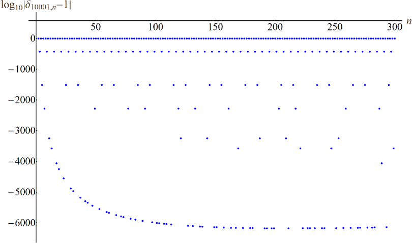
Figure 7: Graph of $\log_{10}|\delta_{10001,n}-1|$.

Here we can observe several horizontal rows of dots. The top row corresponds to even values of $n$ for which $\delta_{10001,n}$ is, according to (22), close to $-1$. The second row corresponds to odd values of $n$ divisible by $3$. The third row corresponds to those values of $n$ that are divisible by $5$ but are relatively prime to $2\cdot 3$. The fourth row corresponds to those values of $n$ that are divisible by $7$ but are relatively prime to $2\cdot 3\cdot 5$, and so on. The seventh row, the last one that we can see, contains only two dots corresponding to $n=17$ and $n=289$.

The remaining dots correspond to prime values of $n$. So we can say that the initial part of the plot of $\log_{10}|\delta_{10001,n}-1|$ represents the Sieve of Eratosthenes. Respectively, the horizontal rows corresponding to the values of $n$ divisible by $2$, by $3$, …but not by the previous primes will be called Eratosthenes levels.

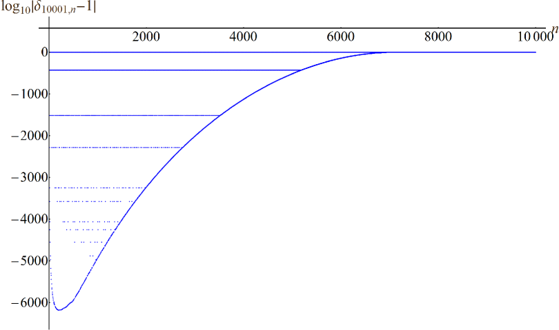
Figure 8: Graph of $\log_{10}|\delta_{10001,n}-1|$.

Figure 8 extends Figure 7 up to $n=10001$. We see that the Eratosthenes levels break off when they touch a mysterious ‘‘smooth curve’’ of increasing values of $\log_{10}|\delta_{10001,n}-1|$. The larger $N$, the more to the right is the smooth curve.

Figure 9 presents results of our computations for $N=12001$. It again shows the Eratosthenes levels but also gives an impression of a new phenomenon – dots corresponding to all primes greater than 80 look like lying on a horizontal line with the ordinate $-7157$. Actually, this is due to the fact that the calculated values of the coefficients have only about 7157 correct decimal digits.

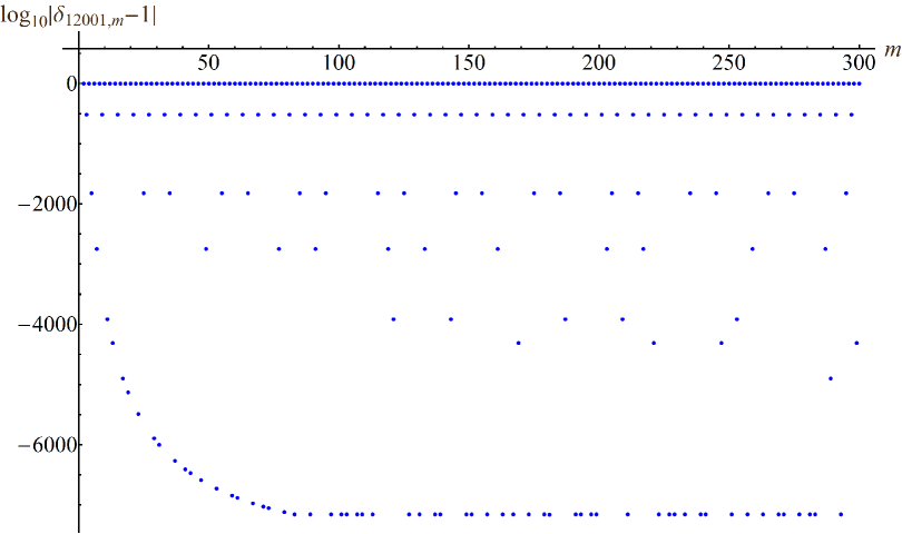
Figure 9: An artifact caused by insufficient accuracy.

6.2 Fractal structure

Figure 10: Graph of $\log_{10}|\delta_{10001,3m}-\delta_{10001,3}|$ showing Eratosthenes sublevels.

The Eratosthenes levels on Figures 7–8 look like lying on straight lines. However, closer examination reveals that each of the levels in its turn contains sublevels corresponding to a slightly modified Sieve of Eratosthenes. Figure 10 shows such sublevels for the main Eratosthenes level corresponding to prime $p=3$ in the case $N=10001$. These sublevels correspond to deleting composite numbers according to their divisibility at first by $2$, then by $5$, $7$, $3$, $11$, $13$, ….

The general rule seems to be as follows. The dots representing $\delta_{N,n}$ for $n$ from an arithmetical progression $d,2d,\dots,md,\dots$ with $d=2^{k_{2}}3^{k_{3}}\dots$ split into Eratosthenes sublevels according to the divisibility of $m$ by $p_{1}$, $p_{2}$, …where these prime numbers are ordered in such a way that

$$p_{1}^{k_{p_{1}}+1}<p_{2}^{k_{p_{2}}+1}<\dots<p_{j}^{k_{p_{j}}+1}<\dots\ .$$ (28)

7 Related and Further Research

Originally, the second author ([Matiyasevich 2012, Matiyasevich 2013] examined the determinants slightly different from those in (16) for which $\Delta^{\Gamma}_{N}(s)$, the counterpart of (10), vanishes at $2N-2$ zeroes of $\zeta(s)$. This becomes possible thanks to the so called functional equation established by Riemann [Riemann 1859]. Properties of $\Delta^{\Gamma}_{N}(s)$ are similar but not the same as those of $\Delta_{N}(s)$. In particular, the Eratosthenes sieve manifests itself not so spectacular. On the other hand, $\Delta^{\Gamma}_{N}(s)$ allows one to calculate approximations not only to the zeroes and the values of the zeta function but to its first derivative as well.

We plan to examine the counterparts of $\delta_{N,n}$ and $\Delta_{N,n}$ for the cases when zeroes of the zeta function are replaced by zeroes of Dirichlet $L$-functions, as well as to perform computations in interval multiprecision arithmetics using Arb [Johansson 2013] to obtain rigorous bounds on the resulting values.

This ongoing research can be followed on [Matiyasevich].

8 Conclusion

We performed large scale high accuracy computations of the coefficients of the finite Dirichlet series approximating nontrivial zeros of Riemann’s zeta function. Our aim was to reveal experimentally new relations between these coefficients and various related quantities, such as the zeros of the alternating zeta function. The results of our computations are somewhat unexpected. Firstly they revealed that the finite Dirichlet series also approximates (with high accuracy) other zeros of zeta function (trivial and subsequent non-trivial zeros), not used in computations. Secondly, the coefficients inconspicuously looking as $+1$ and $-1$ have in fact a rich structure related to prime numbers.

We want to underline the necessity for performing computations with very high accuracy, which was crucial in discovering the patterns presented here, that would not be detected otherwise. The calculations performed were costly, of order of 200,000 CPU hours, which were made possible by collaborative work of mathematicians, computer scientists, programmers and support engineers.

Of course, in Number Theory there are many examples of conjectures that were at first substantiated by calculation for many initial values of the parameters, but then were disproved either theoretically or by finding a numerical counterexample. Nevertheless, we find it highly desirable to extend our calculations to higher sizes of determinants in order to study subtler properties of the intriguing numbers $\delta_{N,n}$. This requires significant computational resources and multi-party collaboration. Our recent experiences with computational aspects of multiprecision calculations are presented in [BeliakovMatiyasevich 2013].

References

- [Bailey 2013] D.H. Bailey. Arprec library http://crd-legacy.lbl.gov/~dhbailey/mpdist/, Accessed June 10, 2013.
- [Balazard et al 2009] M. Balazard, O. V. Castañón. Sur l’infimum des parties réelles des zéros des sommes partielles de la fonction zêta de Riemann. C. R., Math., Acad. Sci. Paris 347, No. 7-8, 343-346 (2009)
- [BeliakovMatiyasevich 2013] G. Beliakov, Yu. Matiyasevich. A Parallel Algorithm for Calculation of Large Determinants with High Accuracy for GPUs and MPI clusters. http://arxiv.org/abs/1308.1536 (2013)
- [BeliakovMatiyasevich 2013a] G. Beliakov and Yu. Matiyasevich. 2013, Zeroes of Riemann’s zeta function on the critical line with 40000 decimal digits accuracy, Research Data Australia, available online http://hdl.handle.net/10536/DRO/DU:30056270
- [Borwein et al 2007] P. Borwein, G. Fee, R. Ferguson and A. van der Waall : Zeros of partial sums of the Riemann zeta function. Experiment. Math., 16(1):21–39, 2007.
- [Chebyshev 1852] P. L. Chebyshev. Memoir sur les nombres premiers. J. Math. Pures Appl., 17, 1852.
- [Euler 1737] L. Euler. Variae observationes circa series infinitas. Commentarii academiae scientarum Petropolitanae 9 (1737), 1744, p. 160 Available on line (including English translation) via http://eulerarchive.maa.org/pages/E072.html
- [GMP] GNU. GNUMP library http://gmplib.org, Accessed June 10, 2013.
- [GonekLedoan 2010] S. M. Gonek and A. H. Ledoan. Zeros of partial sums of the Riemann zeta-function. Int. Math. Res. Not., 2010:10, 1775-1791 (2010)
- [Gourdon 2004] X. Gourdon. The first zeros of the Riemann Zeta function, and zeros computation at very large height. http://numbers.computation.free.fr/Constants/Miscellaneous/zetazeros1e13-1e24.pdf
- [Hilbert 1900] Hilbert D. Mathematische Probleme. Vortrag, gehalten auf dem internationalen Mathematiker Kongress zu Paris 1900. Nachr. K. Ges. Wiss., Göttingen, Math.-Phys. Kl., pages 253–297, 1900. Reprinted in: Arch. Math. Phys. (1901) 44–63, 213–237, and in: Gesammelte Abhandlungen, Berlin : Springer, vol. 3 (1935), 310 (Reprinted: New York : Chelsea (1965)). English translation in: Bull. Amer. Math. Soc. (1901-1902) 437-479. Reprinted in: Mathematical Developments arising from Hilbert Problems, Proceedings of Symposia in Pure Mathematics, vol. 28, American Mathematical Society, Browder Ed., 1976, pp. 1–34.
- [Johansson 2013] F. Johansson. Arb, http://fredrikj.net/arb/
- [Levinson 1973] N. Levinson. Asymptotic Formula for the Coordinates of the Zeros of Sections of the Zeta Function, , Near , 70:4, 985-987 (1973)
- [Mangoldt 1895] H. von Mangoldt. Zu Riemanns Abhandlung ‘Über die Anzhal der Primzahlen unter einer gegebenen Grösse’. J. Reine Agew.Math., 114:255–305, 1985.
- [Matiyasevich] Yu. Matiyasevich. An artless method for calculating approximate values of zeros of Riemann’s zeta function. http://logic.pdmi.ras.ru/~yumat/personaljournal/artlessmethod/artlessmethod.php.
- [Matiyasevich 2012] Yu. Matiyasevich. New conjectures about zeroes of Riemann’s zeta function. Research Reports MA12-03 of The Department of Mathematics of University of Leicester, available online http://www2.le.ac.uk/departments/mathematics/research/research-reports-2/reports-2012/ma12-03, 2012.
- [Matiyasevich 2013] Yu. Matiyasevich. Calculation of Riemann’s zeta function via interpolating determinants. Preprint 2013-18 of Max Planck Institute for Mathematics in Bonn, available online http://www.mpim-bonn.mpg.de/preblob/5368, 2013.
- [MatiyasevichBeliakov 2013] Yu. Matiyasevich and G. Beliakov. 2013, Zeroes of Riemann’s zeta function on the critical line with 20000 decimal digits accuracy, Research Data Australia, available online http://hdl.handle.net/10536/DRO/DU:30051725
- [Montgomery 1983] H. L. Montgomery. Zeros of approximations to the zeta function. In Studies in Pure Mathematics, p. 497–506. Birkhäuser, Basel, 1983.
- [Riemann 1859] B. Riemann. Über die Anzhal der Primzahlen unter einer gegebenen Grösse. Monatsberichter der Berliner Akademie, 1859. Included into: Riemann, B. Gesammelte Werke. Teubner, Leipzig, 1892; reprinted by Dover Books, New York, 1953. http://www.claymath.org/millennium/Riemann_Hypothesis/1859_manuscript/zeta.pdf, English translation http://www.maths.tcd.ie/pub/HistMath/People/Riemann/Zeta/EZeta.pdf.
- [Spira 1966] R. Spira. Zeros of sections of the zeta function, I. Mathematics of Computation, 20, 542–550, (1966)
- [Spira 1968] R. Spira. Zeros of sections of the zeta function, II. Mathematics of Computation, 22, 163–173 (1968)
- [Spira 1972] R. Spira. The lowest zero of sections of the zeta function. Journal für die reine und angewandte Mathematik 255, 170-189, (1972)
- [Turan 1948] P. Turán. On some approximative Dirichlet-polynomials in the theory of the zeta-function of Riemann. Danske Vid. Selsk. Mat.-Fys. Medd., 24(17):36, 1948.
- [Clay] The millennium prize problems. http://www.claymath.org/millennium/.
- [Voronin 1974] С. М. Воронин. О нулях частичных сумм ряда Дирихле дзета-функции Римана. Доклады АН СССР, 216:5, 964-967 (1974). Translated in J. Sov. Math., Dokl. 15, 900-903 (1974).