Plasmonic interferometry: probing launching dipoles in scanning-probe plasmonics

Abstract

We develop a semi-analytical method for analyzing surface plasmon interferometry using near-field scanning optical sources. We compare our approach to Young double hole interferometry experiments using scanning tunneling microscope (STM) discussed in the literature and realize experiments with an aperture near-field scanning optical microscope (NSOM) source positioned near a ring like aperture slit milled in a thick gold film. In both cases the agreement between experiments and model is very good. We emphasize the role of dipole orientations and discuss the role of magnetic versus electric dipole contributions to the imaging process as well as the directionality of the effective dipoles associated with the various optical and plasmonic sources.

I Introduction

Surface plasmons (SPs) BarnesNature2003 ; emrs and NSOM Novotny share a long common historical background which goes back to the birth of both research fields. Indeed, SPs, collective electronic excitations bounded at a metal dielectric interface, belong to the family of electromagnetic waves which are evanescent in the direction normal to the interface. As such, a near field probe located in the vicinity of the metal can be used to either record or excite SP waves. Here we will focus on the application of such a scanning probe to plasmonic interferometry using holes and slits.
First, it is worth reminding that photon STM (PSTM) Novotny was used long ago to probe SP waves externally excited with a tapered fiber tip located in the near field of the plasmon [4-7]. Recently, the method was applied to observe SP interference fringes in Fabry-Perot resonators such as nanowires Ditlbacher and plasmonic corrals [9-11]. The reciprocal regime i.e., the excitation of SP waves with a scanned nano-antenna, is less common but was also reported using NSOM with aperture optical tips Novotny by Hecht et al. Hecht ; 2b . The method was soon applied to observe SP interference fringes inside lithographed cavities 3c ; 3b or between pairs of holes in metal film Sonnichsen . This was also successfully used to launch SPs to excite the luminescence of quantum dots at low temperature brun , thereby entering into the realm of quantum plasmonics. In this context, a new family of active NSOM tips using a single quantum emitter (such as a single Nitrogen vacancy center in a nano-diamond) glued at the apex of an optical tip 12 ; 13 , was recently used to generate quantum SP states propagating along a metal film or inside plasmonic corrals [20-22].
In all these studies the dipolar approximation for describing the electromagnetic field generated by the NSOM tip has been applied with success in agreement with previous optical characterization measurements and models of aperture tips [19,23-26]. SPs launched from such aperture NSOM tips show characteristics dipolar profiles [12,14-17,20,21]. This is reminiscent of the seminal Sommerfeld antenna theory introducing surface waves SommerfeldAP1909 , which was recently extended to thin metal films supporting SP waves launched by point-like radiating dipoles 2b ; NikitinPRL2010 ; Genet . Experimental demonstration in both the near field or far field using the so-called leakage radiation microscopy (LRM) with aperture or active NSOM tips 2b ; 15 ; 19 ; Genet ; 17 confirms these findings, in particular the fact that a NSOM tip behaves essentially as an in-plane radiating dipole.
Interestingly, similar features were obtained using STM tips STM1 ; STM2 . In these experiments, inelastic electrons tunneling through a tip/metal film junction generate photoemission STM3 ; STM4 which, in turn, couples into SPs propagating along the metal/air interface. Modeling of such a system involves a vertical transition dipole aligned with the STM tip revolution axis marty ; STM1 in agreement with LRM images STM1 ; STM2 .
The potentialities of both NSOM and STM scanning sources for plasmonics have however not be fully appreciated despite the fact that these sources provide a natural way for mapping the localized density of states (LDOS) of photonic and plasmonic modes around nanostructures Gerard ; 3 ; 24 . This strongly motivates the present work that is devoted to a better understanding of the interactions between scanning excitation sources and a plasmonic environment. Moreover, due to the precise position control of NSOM or STM tips, this SP excitation method provides a natural way to study SP interferometry different from the PSTM approach [9-11,40,41]. An experiment using a STM tip to launch SP waves in the direction of two subwavelength holes milled in a thick gold film was recently reported sample . The holes, acting together as a pair of coherent sources induced optical fringes in the Fourier plane of a microscope objective. This is reminiscent of previous adaptations of Young double slits experiments with noble metals Gan ; Kuzmin in which a SP contribution was clearly involved in the far-field fringe visibility and phase shift.
In the present work, we study SP interferometry both theoretically and experimentally using an aperture NSOM launching SPs inside a circular corral. We also discuss the recent experiments realized with a STM tip and two subwavelength holes sample and extend our discussion to larger hole diameters. We emphasize the role of polarization and tip dipole orientations on SP interferometry in both configurations. In particular, we show that the method provides an elegant way to discuss experimentally the old problem of the orientation of the aperture dipoles associated with holes or slits in an opaque metal film Rotenberg ; Yin ; Yi . This, we claim, could play an important role in the context of polarization conversion involving an angular momentum exchange between SP modes, photons, and nanostructuration (see for example [11,46-48]).

II Electric and magnetic dipoles as SP launchers

We start with the description of SPs launched by a NSOM or STM tip along a thick metal film. SP modes propagating along a flat interface $z=0$ are inhomogeneous transverse magnetic waves which are completely defined in each medium $j=0,1$ (air and metal) by a characteristic Debye function $\Psi_{\textrm{SP};j}(x,y,z)e^{-i\omega t}$ obeying the usual Helmholtz equation $[\boldsymbol{\nabla}^{2}+k^{2}\varepsilon_{j}]\Psi_{\textrm{SP};j}=0$, where $k=2\pi/\lambda=\omega/c$ is the wavevector in vacuum and $\varepsilon_{j}(k)$ the dielectric permittivity of each medium. From such a SP characteristic function, the electric displacement $\mathbf{D}_{\textrm{SP};j}$ and magnetic (induction) field $\mathbf{B}_{\textrm{SP};j}$ are defined (in the Heaviside system of units) by:

$$\mathbf{D}_{\textrm{SP};j}(x,y,z)=\boldsymbol{\nabla}\times\boldsymbol{\nabla}\times[\mathbf{\hat{z}}\Psi_{\textrm{SP};j}(x,y,z)]$$

$$\mathbf{B}_{\textrm{SP};j}(x,y,z)=-ik\boldsymbol{\nabla}\times[\mathbf{\hat{z}}\Psi_{\textrm{SP};j}(x,y,z)],$$ (1)

$z$ defining the normal direction to the interface and $\mathbf{\hat{z}}$ oriented from the metal side ($z<0$) to the air side ($z>0$). Using boundary conditions at the interface and infinity we write $\Psi_{\textrm{SP};j}(x,y,z)=\Phi_{\textrm{SP}}(x,y,)f_{j}(z)$ where $f_{0}(z)=e^{ik_{0}z}$ and $f_{1}(z)=e^{-ik_{1}z}$ define exponential decays in both media justifying the SP confinement at the interface. Also $\Phi_{\textrm{SP}}(x,y,)$ fulfills the bidimensional Helmoltz equation $[\boldsymbol{\nabla}_{||}^{2}+k^{2}_{\textrm{SP}}]\Phi_{\textrm{SP}}(x,y)=0$ , with $\boldsymbol{\nabla}_{||}=\frac{\partial}{\partial x}\mathbf{\hat{x}}+\frac{\partial}{\partial y}\mathbf{\hat{y}}$ characterized by the usual SP wave vector $k_{\textrm{SP}}=k\sqrt{\frac{\varepsilon_{0}\varepsilon_{1}}{\varepsilon_{0}+\varepsilon_{1}}}=kn_{\textrm{SP}}+i/(2L_{\textrm{SP}})$ ($n_{\textrm{SP}}$ and $L_{\textrm{SP}}$ are respectively the SP effective index and propagation length) together with $k_{j}=\sqrt{k^{2}\varepsilon_{j}-k^{2}_{\textrm{SP}}}$ (to obtain attenuation we impose $\textrm{Imag}[k_{j}]>0$) BarnesNature2003 .
For the present purpose we consider the SP field generated by a point-like dipole located near the interface. A rigorous calculation involves an evaluation of the Sommerfeld integral obtained by continuation in the complex plane 2b ; SommerfeldAP1909 ; Genet , but this goes beyond the purpose of the present paper. Here, we are only interested in the so-called singular or polar contribution which is associated with the propagating SP wave and dominates the far-field NikitinPRL2010 ; Genet . From symmetry considerations we can directly obtain the characteristic Debye potentials $\Phi_{\textrm{SP}}$ (of argument $\mathbf{r}=x\mathbf{\hat{x}}+y\mathbf{\hat{y}}$) for a vertical and horizontal dipole. Using Hankel functions these potentials are respectively:

$$\Phi_{\textrm{SP},\bot}(\mathbf{r})=\eta_{\bot}p_{z}H_{0}^{(+)}(k_{\textrm{SP}}|\mathbf{R}|)$$

$$\Phi_{\textrm{SP},||}(\mathbf{r})=\eta_{||}H_{1}^{(+)}(k_{\textrm{SP}}|\mathbf{R}|)\mathbf{\hat{R}}\cdot\mathbf{p}_{||},$$ (2)

with $p_{z}$ and $\mathbf{p}_{||}$ the vertical, respectively horizontal, dipole components and $\mathbf{R}=\mathbf{r}-\mathbf{r}_{0}$ if the tip is located at $\mathbf{r}_{0}=x_{0}\mathbf{\hat{x}}+y_{0}\mathbf{\hat{y}}$. The coupling constants $\eta_{\bot}=\frac{1}{2}\frac{\varepsilon_{1}^{2}}{\varepsilon_{1}^{2}-\varepsilon_{0}^{2}}e^{ik_{0}h}$ and $\eta_{||}=i\frac{k_{0}}{k_{\textrm{SP}}}\eta_{\bot}$ depend explicitly on the dipole height $z=h$ over the metal surface and are evaluated

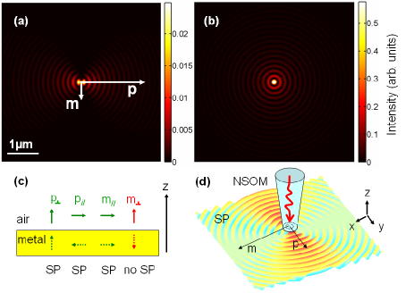
Figure 1: (a), respectively (b): SP intensity field, i.e. $(\textrm{Re}[E_{z}])^{2})$ generated by a point-like horizontal, respectively vertical, dipolar source. In (a) the source can be either an electric or magnetic in-plane dipole. The horizontal, respectively vertical, white arrow represents the direction and relative intensity of the equivalent electric, respectively magnetic, dipoles. In (b) the intensity corresponds to a vertical dipole of same amplitude as the electric dipole of (a). (c): table summarizing the possibility for exciting SPs with dipoles located near a metal film. The dipoles directions and those of their (quasi-static) image dipoles in the thick film are depicted to guide the reasoning. (d): representation of the SP field generated by an aperture NSOM source located near a metal film. The direction of the two effective electric and magnetic dipoles are represented by black arrows. The intensity map corresponds to (a).

using the residue theorem (see also Genet for details).
A few remarks are here relevant: first the coupling constants decay exponentially as $h$ increases showing that one must be very close from the surface in order to excite SP waves. Second, the relation between $\eta_{\bot}$ and $\eta_{||}$ implies that it is much easier to excite SPs with a vertical dipole than with an in-plane dipole since the ratio $\frac{k_{0}}{k_{\textrm{SP}}}$ is in general smaller than one. This agrees with a simple qualitative argument comparing the image dipoles for both configurations. For example, at a wavelength $\lambda=647$ nm for an air/gold interface we obtain $\frac{k_{0}}{k_{\textrm{SP}}}\simeq 0.27$ using $\varepsilon_{0}\simeq 1$, $\varepsilon_{1}\simeq-13.6482+1.0352i$ Johnson . The probability of SP excitation for an horizontal dipole amounts therefore to only $(\frac{k_{0}}{k_{\textrm{SP}}})^{2}=7\%$ of the emission obtained for a vertical dipole of the same amplitude. This is particularly relevant for NV-based NSOM tips [18-22], where the fixed transition dipoles are oriented in a uncontrollable way in the diamond crystal. We also point out that the above analysis is done by assuming the film thickness $d$ large enough to neglect the effect of the second interface emrs , typically $d\gtrsim 70$ nm for gold film. However, the main reasoning keeps its validity for thinner films where leakage radiation is involved. In particular the ratio formulas between $\eta_{||}$ and $\eta_{\bot}$ or $W_{||}$ and $W_{\bot}$ are kept unchanged even though the dispersion relation for $k_{\textrm{SP}}$ is modified emrs .
Most importantly for the present work, we stress that the asymptotic behavior of the singular Hankel functions $H_{0}^{(+)}(k_{\textrm{SP}}|\mathbf{R}|)$ and $H_{1}^{(+)}(k_{\textrm{SP}}|\mathbf{R}|)$ goes like $\frac{e^{ik_{\textrm{SP}}|\mathbf{R}|}}{\sqrt{R}}$ if $R>>\lambda$. Therefore, inserting these expressions in Eq. 1 we obtain the so called Zenneck SP mode: $\mathbf{D}_{\textrm{SP};j}(\mathbf{r},z)\simeq\Phi_{\textrm{SP}}(\mathbf{r})f_{j}(z)\mathbf{g}_{j}$, $\mathbf{B}_{\textrm{SP};j}(\mathbf{r},z)\simeq\Phi_{\textrm{SP}}(\mathbf{r})f_{j}(z)k_{\textrm{SP}}k\mathbf{\hat{R}}\times\mathbf{\hat{z}}$ with $\mathbf{g}_{0}=-k_{\textrm{SP}}k_{0}\mathbf{\hat{R}}+k_{\textrm{SP}}^{2}\mathbf{\hat{z}}$, and $\mathbf{g}_{1}=+k_{\textrm{SP}}k_{1}\mathbf{\hat{R}}+k_{\textrm{SP}}^{2}\mathbf{\hat{z}}$. More generally, using such a Debye potential formalism, it is easy to obtain from Eqs. 1,2 the plasmonic dyadic Green function defined by $\mathbf{D}_{\textrm{SP};j}(\mathbf{r},z)=\overline{\mathbf{G}}_{\textrm{SP}}(\mathbf{r},z,\mathbf{r}_{0},h;j)\cdot\mathbf{p}$ and

$$\overline{\mathbf{G}}_{\textrm{SP}}(\mathbf{r},z,\mathbf{r}_{0},h;j)=\eta_{\bot}f_{j}(z)\{-\delta_{j}ik_{j}k_{\textrm{SP}}$$

$$\cdot H_{1}^{(+)}(k_{\textrm{SP}}|\mathbf{R}|)\hat{\mathbf{R}}\otimes\hat{\mathbf{z}}+k_{\textrm{SP}}^{2}H_{0}^{(+)}(k_{\textrm{SP}}|\mathbf{R}|)\hat{\mathbf{z}}\otimes\hat{\mathbf{z}}$$

$$+i\frac{k_{0}}{k_{\textrm{SP}}}[\delta_{j}ik_{j}k_{\textrm{SP}}\frac{H_{0}^{(+)}(k_{\textrm{SP}}|\mathbf{R}|)-H_{2}^{(+)}(k_{\textrm{SP}}|\mathbf{R}|)}{2}\hat{\mathbf{R}}\otimes\hat{\mathbf{R}}$$

$$+\frac{H_{1}^{(+)}(k_{\textrm{SP}}|\mathbf{R}|)}{R}\hat{\mathbb{\phi}}\otimes\hat{\mathbb{\phi}}]+ik_{0}k_{\textrm{SP}}H_{1}^{(+)}(k_{\textrm{SP}}|\mathbf{R}|)\hat{\mathbf{z}}\otimes\hat{\mathbf{R}}\}$$ (3)

with $\hat{\mathbb{\phi}}=\hat{\mathbf{z}}\times\hat{\mathbf{R}}$, and $\delta_{0}=-\delta_{1}=1$.
In the context of this work it is relevant to consider the emission associated with a magnetic dipole since it is well known that an aperture NSOM tip radiates like a coherent superposition of in-plane electric and magnetic dipoles $\mathbf{p}_{||,\textrm{aperture}}$ and $\mathbf{m}_{||,\textrm{aperture}}=2\mathbf{p}_{||,\textrm{aperture}}\times\hat{\mathbf{z}}$, with the electric dipole oriented along the electromagnetic mode polarization at the tip apex [19,23-26]. The SP Debye potential associated with a radiating point-like magnetic dipole can be easily obtained from Eq. 2. First, we slightly generalize Eq. 2 to describe a current distribution $\mathbf{J}(\mathbf{r^{\prime}},z^{\prime})=-i\omega\mathbf{P}(\mathbf{r^{\prime}},z^{\prime})$ and obtain: $\Phi_{\textrm{SP};j}(\mathbf{r})=\int d^{2}\mathbf{r^{\prime}}dz^{\prime}\eta_{\bot}(z^{\prime})[H_{0}^{(+)}(k_{\textrm{SP}}|\mathbf{R}|)\mathbf{\hat{z}}\cdot\frac{\mathbf{J}(\mathbf{r^{\prime}},z^{\prime})}{-i\omega}+i\frac{k_{0}}{k_{\textrm{SP}}}H_{1}^{(+)}(k_{\textrm{SP}}|\mathbf{R}|)\mathbf{\hat{R}}\cdot\frac{\mathbf{J}(\mathbf{r^{\prime}},z^{\prime})}{-i\omega}]$, with $\mathbf{R}=\mathbf{r}-\mathbf{r}^{\prime}$, and where the explicit dependence of $\eta_{\bot}(z^{\prime})$ over $z^{\prime}$ is taken into account. Second, we consider a magnetic loop, or equivalently, a current distribution $\mathbf{J}(\mathbf{r^{\prime}},z^{\prime})=c\nabla^{\prime}\times\mathbf{M}(\mathbf{r^{\prime}},z^{\prime})$, where $\mathbf{M}$ is the magnetic dipole distribution. After integration by parts and use of the point-like dipole limit: $\mathbf{M}(\mathbf{r^{\prime}},z^{\prime})=\mathbf{m}\delta^{2}(\mathbf{r^{\prime}}-\mathbf{r}_{0})\delta(z^{\prime}-h)$ we obtain

$$\Phi_{\textrm{SP}}(\mathbf{r})=-i\frac{k}{k_{\textrm{SP}}}\eta_{\bot}H_{1}^{(+)}(k_{\textrm{SP}}|\mathbf{R}|)\mathbf{\hat{\phi}}\cdot\mathbf{m}_{||}.$$ (4)

A few points are here remarkable. First, we find that for a vertical magnetic dipole the SP field vanishes, a very fact that qualitatively agrees with the symmetry of the magnetic field $B_{z}\neq 0$ associated with a vertical magnetic dipole, which cannot couple to transverse magnetic waves, i.e., SPs for which $B_{z}=0$. Second, and this is very important in the NSOM context, Eq. 4 is equivalent to Eq. 2 if we define an effective electric dipole $\mathbf{p}_{||,\textrm{eff.}}=\frac{k}{k_{0}}\hat{\mathbf{z}}\times\mathbf{m}_{||}$ since $-\mathbf{\hat{\phi}}\cdot\mathbf{m}_{||}=\frac{k_{0}}{k}\mathbf{\hat{R}}\cdot\mathbf{p}_{||,\textrm{eff.}}$. In other words it is not possible to distinguish the SP field created by an in-plane magnetic dipole $\mathbf{m}_{||}$ from the one created by an in-plane electric dipole $\mathbf{p}_{||,\textrm{eff.}}$ obtained by rotating $\mathbf{m}_{||}$ by $\pi/2$ around the $z$ axis. We think that this difficulty could be of particular importance in the context of measurements aiming at determining the dipole orientation of, e.g., a single nanohole drilled through a metal film Rotenberg . Finally, due to the coefficient $\frac{k}{k_{0}}$ in the definition of $\mathbf{p}_{||,\textrm{eff.}}$ we see that in general it is much easier to launch a SP field with an in-plane magnetic dipole than with an electric dipole of the same amplitude. For example at $\lambda=647nm$ using the previous value for $\varepsilon_{1}(k)$ Johnson we get on a semi infinite gold film $(\frac{k}{k_{0}})^{2}\simeq(3.56)^{2}\simeq 12.7$. This is also in qualitative agreement with the image dipole picture in which the in-plane magnetic dipole and its image enforce each other while they tend to compensate in the electric dipole case. Now, for the NSOM tip we have a magnetic and an electric dipole orthogonal to each other [19,23-26]. Therefore, the total SP field created by such a tip is equivalent to the field generated by an electric dipole $\mathbf{p}_{||,\textrm{total}}=\mathbf{p}_{||,\textrm{aperture}}+\mathbf{p}_{||,\textrm{eff.}}=(1+2\frac{k}{k_{0}})\mathbf{p}_{||,\textrm{aperture}}$. This agrees with experimental measurements of the SP radiation profile for such a source [12,14-17,20,21].
To conclude this section we illustrate all discussed features in Figs. 1 (a) and 1(b) where we computed the SP intensity (here $(\textrm{Re}[E_{z}])^{2})$ along the air-metal interface for respectively an horizontal electric dipole, an equivalent magnetic dipole (as given by Eq. 4) and a vertical dipole. The selection rules for exciting SPs are reminded in Fig. 1 (c) together with the image dipole picture. Finally the SP field associated with an NSOM tip is shown in Fig. 1 (d) together with the aperture dipole directions.

III Plasmonic interferometry with a STM tip source

As a direct application we now analyze in more detail the experimental configuration of ref. sample , where a STM tip was used to excite SP waves on a 200 nm thick gold film. This film was milled

Figure 2: Finite element simulation of the electromagnetic field diffracted by a single cylindrical subwavelength aperture in a thick gold film. The incident light mode is a pure SP wave with in-plane wavevector aligned with the x axis (red arrow). (a) and (b) are intensity maps in the x-z plane. (c) and (d) correspond to intensity maps in the x-y plane ($z=-200$ nm). (a) and (c) are maps of the total electric intensity $|\mathbf{E}(x,y,z)|^{2}$, whereas (b) and (d) correspond to the magnetic intensity $|\mathbf{B}(x,y,z)|^{2}$.

with two 250 nm-diameter holes separated by a distance of $d_{12}=2\mu$m. In this experiment these holes acted as two coherent nano-sources of light which subsequently interfered in the back-focal plane of a high NA microscope objective.
Let us first consider an isolated hole. Diffraction by single hole in a metal film is a difficult theoretical problem with a long history [50-52], which was recently renewed in the context of plasmonics NikitinPRL2010 ; Rotenberg ; Yi ; Bonod . In order to visualize the diffracted electromagnetic field in the vicinity of the hole when a SP wave impinges on it, we first simulated the problem by using a finite element analysis software [Comsol Multiphysics] at the optical wavelength $\lambda=647$ nm for the material and geometry parameters of the STM experiment sample . The results are shown in Fig. 2 for both the total electric and magnetic field intensity $|\mathbf{E}|^{2}$ and $|\mathbf{B}|^{2}$. The incident SP wave used in this simulation is a rigorous mode of the air-metal-glass multilayer medium. As explained in ref. Genet ; emrs we consider here a leaky mode mainly confined along the air-metal interface (i.e. $z=0$), which is growing exponentially in the substratum and has an in-plane wavevector $\textbf{k}_{\textrm{SP}}$ aligned along the +$x$ direction (direction indicated by a red arrow in Fig. 2). From the images in Figs. 2(a) and 2(b) we see that the transmitted field is strongly damped through the hole. This is reminiscent of previous studies of transmission by holes, where only the fundamental mode (i.e. in general the transverse electric mode $\textrm{TE}_{11}$ Yi ) is excited. Here however, the incoming SP is a pure TM wave and therefore the coupling with TM modes cannot be neglected. Comparing the magnetic and electric intensity images we see that $|\mathbf{E}|^{2}\sim|\mathbf{B}|^{2}$, in opposition with results obtained with an incident propagating light wave instead of a SP mode (compare for example with Fig. 1 of ref. Kim5 ). This will naturally imply a different expansion into multipoles as for the usual Bethe diffraction formula Yi ; Bethe ; Roberts (see for example Rotenberg , in which the vertical component electric dipole $p_{z}$ plays a fundamental role). Finally, the intensity profiles in the exit aperture plane (i.e. $z=-200$ nm) reveal symmetries along the privileged direction defined by the SP wavevector but no clear dominance of the magnetic field over the electric field (see Figs. 2(c) and 2(d)) despite the fact that the electric field is strongly confined near the rim of the hole. This again stresses the fact that with SPs as excitation of single holes, both the magnetic and electric components play an important role.
It is beyond the aim of the present work to give a full discussion of the SP diffraction problem by hole(s). Here, we instead emphasize simple arguments adapted to our specific problem. We will use a semi-analytical approach based on the Green Dyadic tensor formalism.
For this purpose we remind that the electric displacement field $\mathbf{D}(M)$ at point $M$ in the region surrounding the hole is given by a Lippman Schwinger integral $\mathbf{D}(M)=\mathbf{D}_{\textrm{SP}}(M)+\int_{V}d^{3}x^{\prime}\bar{\textbf{G}}_{\textrm{film}}(M,M^{\prime})(\varepsilon_{0}-\varepsilon_{1})\mathbf{E}(M^{\prime})$ where $\bar{\textbf{G}}_{\textrm{film}}(M,M^{\prime})$ is the total dyadic Green tensor corresponding to the film without hole, the integration volume $V$ corresponds to the cylindrical region occupied by the hole (filled with air) and $\mathbf{D}_{\textrm{SP}}(M)$ is the incident SP field propagating along the interface $z=0$ and existing without the hole NikitinPRL2010 ; Yi . In the transmitted region $z<-d$, $\mathbf{D}_{\textrm{SP}}(M)\approx 0$ and only the volume integral survives. Now, to first-order (Born) approximation, we can write in the transmitted region $\mathbf{D}(M)\simeq\int_{V}d^{3}x^{\prime}\bar{\textbf{G}}_{\textrm{film}}(M,M^{\prime})(\varepsilon_{0}-\varepsilon_{1})\mathbf{E}_{\textrm{SP}}(M^{\prime})$, where $\mathbf{E}_{\textrm{SP}}$ is the incident unperturbed SP field. However, since the SP field strongly decays in the metal (since $1/(2\textrm{Imag}k_{1})\simeq 10nm$) the volume integral evolves into a surface integral over the aperture area $S$: $\mathbf{D}(M)\simeq\frac{i}{k_{1}}\int_{S}d^{2}\mathbf{r}^{\prime}\bar{\textbf{G}}_{\textrm{film}}(M,\mathbf{r}^{\prime},z^{\prime}=0^{-})(\varepsilon_{0}-\varepsilon_{1})\mathbf{E}_{\textrm{SP}}(\mathbf{r}^{\prime},z^{\prime}=0^{-})$, where the coefficient $\frac{i}{k_{1}}$ arises from an integration of the SP exponential decay $\int^{0}_{-h}dzf_{1}(z^{\prime})\simeq\int^{0}_{-\infty}dzf_{1}(z^{\prime})=i/k_{1}$. Importantly, contrary to what occurs in air, the SP field in the metal is dominated by its tangential components since $|E_{z}|/|E_{t}|\simeq|k_{\textrm{SP}}/k_{1}|\simeq 0.27$ for the same material parameter as before. Therefore, for small radius $a$ the hole acts essentially as an in-plane dipole $\mathbf{p}_{\textrm{hole}}\simeq\frac{i(\varepsilon_{0}-\varepsilon_{1})}{k_{1}}\int_{S}d^{2}x^{\prime}\mathbf{E}_{\textrm{SP}}(\mathbf{r}^{\prime},z^{\prime}=0^{-})$ leaking through the metal film and located on the interface $z=0$. We point out that this first-order approximation could lead to some problems at large diffraction angle where it is known that leaky photons can couple to SPs at the specific angle $\theta_{\textrm{LR}}=\arcsin{(n_{\textrm{SP}}/n)}$ emrs ; Genet . However, we will neglect this point here and will consider that for horizontal dipoles, the dominant contribution is associated with the radiative part occurring below the total internal reflection angle $\theta_{c}=\arcsin{(1/n)}$.
In the next stage, to describe the diffracted field one must also take into account the hole size and retardation effects. For this purpose, consider now a point-like dipole $\mathbf{p}$ located in the hole and radiating light in free space in the direction of the microscope objective. The electric field measured at a distance $S=\textrm{OM}\gg\lambda$ of the plane $z=0$ takes the asymptotic form $\mathbf{E}(t)\simeq\textrm{const.}\frac{p(t-nS/c)}{S}[\mathbf{\hat{p}}-(\mathbf{\hat{p}}\cdot\mathbf{\hat{S}})\mathbf{\hat{S}}]$, where $\mathbf{\hat{S}}=\mathbb{OM}/|\mathbb{OM}|$ is the unit vector directed from the hole center O to the observation point M and $n$ is the optical index of the substrate (this formula is justified since the asymptotic part of $\bar{\textbf{G}}_{\textrm{film}}$ for observation points not too far from the optical axis $-z$ approaches the dyadic for the substratum of permittivity $n^{2}$). From the previous discussion it should now be clear that the aperture as a whole acts as a coherent integral distribution of such dipoles excited by the incident (in-plane) SP field $\mathbf{E}_{\textrm{SP}}$ impinging on the hole. The total field at the observation point reads consequently $\mathbf{E}=\textrm{const.}\frac{e^{iknS}}{S}\mathbf{Q}[\mathbf{k}_{||}]$, where $\mathbf{Q}[\mathbf{k}_{||}]$ is the structure factor defined by

$$\mathbf{Q}[\mathbf{k}_{||}]=\int_{S}d^{2}\mathbf{r}^{\prime}e^{-i\mathbf{k}_{||}\cdot\mathbf{r}^{\prime}}[\mathbf{E}_{\textrm{SP}}(\mathbf{r}^{\prime})-(\mathbf{E}_{\textrm{SP}}(\mathbf{r}^{\prime})\cdot\mathbf{\hat{S}})\mathbf{\hat{S}}]$$ (5)

calculated for the special in-plane wavevector $\mathbf{k}_{||}=kn[(\mathbf{\hat{S}}\cdot\mathbf{\hat{x}})\mathbf{\hat{x}}+(\mathbf{\hat{S}}\cdot\mathbf{\hat{y}})\mathbf{\hat{y}}]$. Suppose for example an incident SP wave $\mathbf{E}_{\textrm{SP},||}(\mathbf{r}^{\prime})=\mathbf{\hat{u}}e^{ik_{\textrm{SP}}\mathbf{\hat{u}}\cdot\mathbf{r}^{\prime}}$ (i.e., considering only in-plane components of the SP field), and a cylindrical hole centered on the in-plane vector $\mathbf{r}_{0}=x_{0}\mathbf{\hat{x}}+y_{0}\mathbf{\hat{y}}$ we deduce

$$\mathbf{Q}[\mathbf{k}_{||};\mathbf{\hat{u}},\mathbf{r}_{0}]=[\mathbf{\hat{u}}-(\mathbf{\hat{u}}\cdot\mathbf{\hat{S}})\cdot\mathbf{\hat{S}}]2\pi a^{2}e^{-i\mathbf{k}_{||}\cdot\mathbf{r}_{0}}\frac{J_{1}(va)}{va}$$ (6)

with $v=|\mathbf{k}_{||}-k_{\textrm{SP}}\mathbf{\hat{u}}|$ (here we neglected the effect of the SP propagation length $L_{\textrm{SP}}\simeq 10$ $\mu$m in the integration since the hole diameter $2a$ is supposed to be much smaller).
Finally, a rigorous description of the diffracted field requires to consider the electromagnetic field distortion induced by the propagation through the objective. This effect is expected to be small for paraxial light rays propagating close to the optical axis (i.e. in the $-z$ direction) but cannot be neglected in general with high NA objectives. For this purpose, we apply the general Debye procedure described for example in refs. Genet ; Sheppard that consists in introducing a projection condition from the spherical wave front going away from the sample plane onto a planar wave front transmitted by the infinity corrected aplanatic objective. For the source considered here the field on this spherical wave front just before the transformation is collinear to $\mathbf{\hat{u}}-(\mathbf{\hat{u}}\cdot\mathbf{\hat{S}})\cdot\mathbf{\hat{S}}$ , which can also be written as $(\mathbf{\hat{u}}\cdot\mathbf{\hat{\theta}})\mathbf{\hat{\theta}}+(\mathbf{\hat{u}}\cdot\mathbf{\hat{\phi}})\mathbf{\hat{\phi}}$ using the spherical coordinate basis $[S,\theta,\phi]$. This vector is clearly tangential to the sphere, as it should be for far-field radiation. The projection on the planar wave front transforms this vector into $\frac{[((\mathbf{\hat{u}}\cdot\mathbf{\hat{\rho}})\cos{\theta}-(\mathbf{\hat{u}}\cdot\mathbf{\hat{z}})\sin{\theta})\mathbf{\hat{\rho}}+(\mathbf{\hat{u}}\cdot\mathbf{\hat{\phi}})\mathbf{\hat{\phi}}]}{\sqrt{(\cos{(\theta)})}}$ and the square root $\sqrt{(\cos{(\theta)})}$ is introduced to ensure energy conservation during propagation Sheppard . Therefore, using this relation, Eq. 6 must now be replaced by

$$\mathbf{Q^{\prime}}[\mathbf{k}_{||};\mathbf{\hat{u}},\mathbf{r}_{0}]=[((\mathbf{\hat{u}}\cdot\mathbf{\hat{\rho}})\cos{\theta}-(\mathbf{\hat{u}}\cdot\mathbf{\hat{z}})\sin{\theta})\mathbf{\hat{\rho}}$$

$$+(\mathbf{\hat{u}}\cdot\mathbf{\hat{\phi}})\mathbf{\hat{\phi}}]\frac{2\pi a^{2}e^{-i\mathbf{k}_{||}\cdot\mathbf{r}_{0}}}{\sqrt{(\cos{(\theta)})}}\frac{J_{1}(va)}{va}$$ (7)

where $\mathbf{k}_{||}=kn\sin{\theta}\mathbf{\hat{\rho}}$. The electric field in the back-focal plane of the objective (Fourier plane) reads consequently $\mathbf{E}=\textrm{const'.}\frac{e^{iknf}}{f}\mathbf{Q}^{\prime}[\mathbf{k}_{||};\mathbf{\hat{u}},\mathbf{r}_{0}]$ where $f$ is the radius of the spherical wave front (reference sphere), which corresponds to the focal length of the objective.
We now go back to the STM experiment considered in ref. sample and suppose two holes located at $\mathbf{r}_{1}=x_{1}\mathbf{\hat{x}}+y_{1}\mathbf{\hat{y}}$ and $\mathbf{r}_{2}=x_{2}\mathbf{\hat{x}}+y_{2}\mathbf{\hat{y}}$ on the metal film while the STM tip is located at $\mathbf{r}_{0}=x_{0}\mathbf{\hat{x}}+y_{0}\mathbf{\hat{y}}$. SPs launched from the tip to both apertures take the asymptotic form $\textbf{E}_{\textrm{SP},1}\propto\frac{\mathbf{r}_{1}-\mathbf{r}_{0}}{|\mathbf{r}_{1}-\mathbf{r}_{0}|}\frac{e^{ik_{\textrm{SP}}|\mathbf{r}_{1}-\mathbf{r}_{0}|}}{\sqrt{|\mathbf{r}_{1}-\mathbf{r}_{0}|}}$, and $\textbf{E}_{\textrm{SP},2}\propto\frac{\mathbf{r}_{2}-\mathbf{r}_{0}}{|\mathbf{r}_{2}-\mathbf{r}_{0}|}\frac{e^{ik_{\textrm{SP}}|\mathbf{r}_{2}-\mathbf{r}_{0}|}}{\sqrt{|\mathbf{r}_{2}-\mathbf{r}_{0}|}}$ for holes 1 and 2 respectively (the vertical component of the SP fields are not considered here in agreement with our previous discussion).

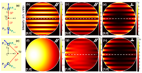
Figure 3: Theoretical modeling of the SP excitation of two subwavelength apertures by a STM tip. The first line (b-d) gives intensity maps of the diffracted intensity detected in the back-focal (Fourier) plane of the high NA objective (here $NA=1.4$) corresponding to the configuration sketched in (a) when the STM tip is located midway between the holes. The second line (f-h) corresponds to the configuration shown in (e). The blue, respectively green, arrows in (a) and (e) represent the direction of horizontal, respectively, vertical electric dipoles associated with the holes. Images (b), (c), (f) and (g) correspond respectively to the horizontal and vertical dipole case. The white dashed lines along the $k_{x}$ axis shows the minimum or maximum fringe intensity.

The total electric field in the back-focal plane of the objective is thus proportional to

$$\textbf{E}(\mathbf{k}_{||})\propto\frac{e^{ik_{\textrm{SP}}|\mathbf{r}_{1}-\mathbf{r}_{0}|}}{\sqrt{|\mathbf{r}_{1}-\mathbf{r}_{0}|}}\mathbf{Q^{\prime}}[\mathbf{k}_{||};\frac{\mathbf{r}_{1}-\mathbf{r}_{0}}{|\mathbf{r}_{1}-\mathbf{r}_{0}|},\mathbf{r}_{1}]$$

$$+\frac{e^{ik_{\textrm{SP}}|\mathbf{r}_{2}-\mathbf{r}_{0}|}}{\sqrt{|\mathbf{r}_{2}-\mathbf{r}_{0}|}}\mathbf{Q^{\prime}}[\mathbf{k}_{||};\frac{\mathbf{r}_{2}-\mathbf{r}_{0}}{|\mathbf{r}_{2}-\mathbf{r}_{0}|},\mathbf{r}_{2}].$$ (8)

The intensity recorded in the back-focal plane is finally obtained as $I(\mathbf{k}_{||})\propto|\mathbf{E}|^{2}$. This takes a simple analytical form for small $\pi-\theta$, i.e., near the optical axis $-z$, and in the limit of small radius $a$ for which the Airy function $\frac{2J_{1}(va)}{va}\simeq 1$. Indeed, in that case, we get

$$I(\mathbf{k})\propto\frac{e^{-R_{1}/L_{\textrm{SP}}}}{R_{1}}+\frac{e^{-R_{2}/L_{\textrm{SP}}}}{R_{2}}$$

$$+2\frac{\mathbf{\hat{R}}_{1}\cdot\mathbf{\hat{R}}_{2}}{\sqrt{R_{1}R_{2}}}e^{-\frac{R_{1}+R_{2}}{2L_{\textrm{SP}}}}\cos{[\mathbf{k}_{||}\cdot\mathbf{d}_{12}+kn_{\textrm{SP}}(R_{2}-R_{1})]}$$ (9)

with $\mathbf{R}_{1}=\mathbf{r}_{1}-\mathbf{r}_{0}$, $\mathbf{R}_{2}=\mathbf{r}_{2}-\mathbf{r}_{0}$ and $\mathbf{d}_{12}=\mathbf{r}_{1}-\mathbf{r}_{2}$.
As an illustration, we now consider the two cases sketched in Fig. 3(a) and 3(e) where:
i) $\mathbf{R}_{1}=-\mathbf{R}_{2}$, i.e., the tip is located along the line joining the holes at mid-way from each (Fig. 3(a)).
ii) The vectors $\mathbf{R}_{1}$ and $\mathbf{R}_{2}$ are orthogonal and equal in norms (Fig. 3 (e)).
In configuration i) the fringe visibility predicted by Eq. 9 is maximal in norm: $V=-1$ while the phase shift $\Delta\phi=kn_{\textrm{SP}}(R_{2}-R_{1})$ vanishes. Oppositely, in configuration ii) Eq. 9 predicts no interference since the fringes visibility vanishes. This result is reproduced by the simulation taking into account the full expression of $\mathbf{Q}[\mathbf{k}_{||};\mathbf{\hat{u}}]$ (Eq. 6) as shown in Figs. 3(b) and 3(f). This corresponds to the intensity that would be measured before the transmission by the objective, i.e., for observation points confined on the reference sphere of radius $f$. This could be experimentally recorded using a goniometer Karrai2 ; Yi . In particular, while there is no interference for case ii) (see Fig. 3(f)) the value $V=-1$ in case i) imposes an interference fringe minimum along the axis $k_{y}=0$ (the white dashed line in Fig. 3(b)), in agreement with the simplified model discussed above. The same features are also observed in the back-focal objective plane if we consider $\mathbf{Q^{\prime}}[\mathbf{k}_{||};\mathbf{\hat{u}},\mathbf{r}]$ instead of $\mathbf{Q}[\mathbf{k}_{||};\mathbf{\hat{u}},\mathbf{r}]$, i.e. Eqs. 7,8 (see Figs. 3(c) and (g)). The distortions observed in Fig. 3(g) compared to Fig. 3(f) are related to the mixing between the polarization induced by the microscope objective and there is now a small fringe minimum along the axis $k_{y}=0$ (white dashed line in Fig. 2(g)).
For comparison, we also show the simulated images in the Fourier space for the case ii) if the holes are supposed to react like vertical dipoles instead of horizontal dipoles (i.e. Figs. 3(d) and 3(h)). In analogy with the discussion leading to Eq. 6 this means that the hole is now driven by the vertical component of the incoming SP: $\mathbf{E}_{\textrm{SP},\bot}(\mathbf{r}^{\prime})=\mathbf{\hat{z}}e^{ik_{\textrm{SP}}\mathbf{\hat{u}}\cdot\mathbf{r}^{\prime}}$. This situation is automatically predicted using Eqs. 6,7 and replacing $\mathbf{\hat{u}}_{1}$, $\mathbf{\hat{u}}_{2}$ by the direction $\mathbf{\hat{z}}$ everywhere but in the definition of $v$. In particular using the same approximations as in Eq. 9 we find that the intensity should vanish in the paraxial regime since to zero order $\mathbf{\hat{z}}\sim\mathbf{\hat{S}}$ and $\mathbf{\hat{z}}-(\mathbf{\hat{z}}\cdot\mathbf{\hat{S}})\cdot\mathbf{\hat{S}}\simeq 0$. A more precise calculation imposing only $\frac{2J_{1}(va)}{va}\simeq 1$ however naturally leads to

$$I(\mathbf{k})\propto\frac{(\sin{\theta})^{2}}{\cos{\theta}}\{\frac{e^{-R_{1}/L_{\textrm{SP}}}}{R_{1}}+\frac{e^{-R_{2}/L_{\textrm{SP}}}}{R_{2}}$$

$$+2\frac{1}{\sqrt{R_{1}R_{2}}}e^{-\frac{R_{1}+R_{2}}{2L_{\textrm{SP}}}}\cos{[\mathbf{k}_{||}\cdot\mathbf{d}_{12}+kn_{\textrm{SP}}(R_{2}-R_{1})]}\}$$ (10)

in the back-focal plane of the objective. This is confirmed by the complete simulation using an adapted structure factor, i.e., replacing Eq. 7 in Eq. 8 by $\mathbf{Q^{\prime\prime}}[\mathbf{k}_{||};\mathbf{\hat{z}},\mathbf{\hat{u}},\mathbf{r}]=\frac{[-\sin{\theta}\mathbf{\hat{\rho}}]}{\sqrt{(\cos{(\theta)})}}2\pi a^{2}e^{-i\mathbf{k}_{||}\cdot\mathbf{r}_{0}}\frac{J_{1}(va)}{va}$ (as shown in Figs. 3d and 3h). Importantly, we find in both cases i) and ii) a residual visibility along the axis $k_{y}=0$, visible only at large $\theta$, due to the optical distortion through the microscope (i.e., the $\sin{\theta}^{2}$ term).
Therefore, we conclude this section by suggesting that the STM SP point source used in refs. STM1 ; STM2 ; sample constitutes an ideal system for probing the dipole orientations associated with diffracting holes in a thick metal film.

IV Plasmonic interferometry with a NSOM tip source

In the case of a NSOM SP source the previous configuration with two holes is not ideal since the in-plane dipoles, either electric or magnetic, associated with the tip aperture introduce an additional degree of freedom which can affect the fringe visibility in the back-focal plane of the microscope. Here, rather than a pair of holes, we consider a circular slit of diameter $D=3,4$ or $5$ $\mu$m and width $w=250$ nm milled in a 200 nm thick gold film: see Figs. 4(a), 4(b), and 4(c), respectively. This circular symmetry restores the symmetry lost with the replacement of the vertical tip dipole by two in-plane orthogonal dipoles. In order to give a detailed description of what is going on when the NSOM tip is located at $\mathbf{r}_{0}=x_{0}\mathbf{\hat{x}}+y_{0}\mathbf{\hat{y}}$ inside this circular corral we first parameterize any point along the aperture rim of radius $D/2$ by $\mathbf{r}(\beta)=(D/2)[\cos{\beta}\mathbf{\hat{x}}+\sin{\beta}\mathbf{\hat{y}}]$ with $\beta\in[0,2\pi[$. As shown by Eqs. 2 or 3, the SP field generated at such a running point by the equivalent electric dipole $\mathbf{p}_{||,\textrm{total}}$ associated with the tip takes the asymptotic form $\mathbf{E}_{\textrm{SP}}\propto\frac{e^{ik_{\textrm{SP}}|\mathbf{R}(\beta)|}}{\sqrt{|\mathbf{R}(\beta)|}}(\mathbf{p}_{||,\textrm{total}}\cdot\mathbf{\hat{R}}(\beta))\mathbf{\hat{R}}(\beta))$ with $\mathbf{R}(\beta)=\mathbf{r}(\beta)-\mathbf{r}_{0}$ (the different vectors involved in this analysis are represented in Fig. 4(c) for clarity).
Now, in contrast with a single hole, a single slit reacts anisotropically to an incoming SP wave. Indeed, it has been shown experimentally that a linear slit acts as a polarizer transmitting or scattering light only if the incoming in-plane SP wavevector $\mathbf{k}_{\textrm{SP}}$ is normal to the slit (see e.g. BaudrionPRB ; Degiron ). This has also been confirmed with circular slits to tailor specific polarization convertors Lombard ; Drezetpola . Here, it implies that each running point $\mathbf{r}(\beta)$ acts a dipole transmitting light in the direction $\mathbf{\hat{r}}(\beta)$ with an amplitude proportional to the scalar product $\mathbf{\hat{R}}(\beta)\cdot\mathbf{\hat{r}}(\beta)$ in agreement with Malus’s law. Therefore, by linear superposition of all these point-like sources, i.e. after integration over $\beta$, we get for the field recorded in the back-focal plane:

$$\textbf{E}(\mathbf{k}_{||})=\textrm{const.}\oint\frac{e^{ik_{\textrm{SP}}|\mathbf{R}(\beta)|}}{\sqrt{|\mathbf{R}(\beta)|}}(\mathbf{p}_{||,\textrm{total}}\cdot\mathbf{\hat{R}}(\beta))$$

$$\mathbf{Q^{\prime}}[\mathbf{k}_{||};(\mathbf{\hat{R}}(\beta)\cdot\mathbf{\hat{r}}(\beta))\mathbf{\hat{r}}(\beta),\mathbf{r}(\beta)]d\beta$$ (11)

in complete analogy with Eq. 8.
We

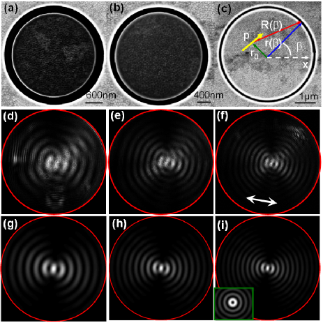
Figure 4: SP excitation of a ring like aperture by a NSOM tip. (a-c) show FIB images of the sample considered with ring diameters 3, 4 and 5 $\mu$m. The directions of the vectors used in the mathematical model are shown in (c). (d-f) are intensity maps in the Fourier plane and correspond to samples (a-c) when the tip is located nearly at the ring cavity center. (g-i) are the associated calculated images for the equivalent horizontal electric NSOM dipole indicated by a double white arrow. The inset in (i) shows what would be observed with a STM tip (images are at the same scale).

consider first the case where the NSOM tip is at the center of the cavity. In that situation the recorded electric field can be approximately evaluated if we write $\mathbf{\hat{u}}-(\mathbf{\hat{u}}\cdot\mathbf{\hat{S}})\cdot\mathbf{\hat{S}}\simeq\mathbf{\hat{u}}$ (paraxial ray approximation) in Eq. 6 or 7. We obtain

$$\textbf{E}(\mathbf{k}_{||})=\textrm{const.}\frac{\pi\sqrt{2}e^{ik_{\textrm{SP}}D/2}}{\sqrt{D}}\{[J_{0}(k_{||}D/2)$$

$$-J_{2}(k_{||}D/2)((\hat{\mathbf{k}}_{||}\cdot\mathbf{\hat{p}}_{||})^{2}-(\hat{\mathbf{k}}_{||}\times\mathbf{\hat{p}}_{||})^{2})]\hat{\mathbf{k}}_{||}$$

$$-2J_{2}(k_{||}D/2)(\hat{\mathbf{k}}_{||}\cdot\mathbf{\hat{p}}_{||})(\hat{\mathbf{k}}_{||}\cdot(\hat{\mathbf{z}}\times\mathbf{\hat{p}}_{||}))\hat{\mathbf{z}}\times\mathbf{\hat{p}}_{||}\}$$

i.e.,

$$\textbf{E}(\mathbf{k}_{||})\simeq\textrm{const.}\frac{\pi\sqrt{2}e^{ik_{\textrm{SP}}D/2}}{\sqrt{D}}\{[J_{0}(k_{||}D/2)$$

$$-J_{2}(k_{||}D/2)\cos{(2\phi)}]\hat{\mathbf{x}}-J_{2}(k_{||}D/2)\sin{(2\phi)}\hat{\mathbf{y}}\}$$ (13)

where $\mathbf{k}_{||}=k_{||}(\cos{\phi}\hat{\mathbf{x}}+\sin{\phi}\hat{\mathbf{y}})$. In going from Eq. 12 to 13 we imposed $\mathbf{\hat{p}}_{||}$ to simplify the mathematical expression (i.e. the equivalent NSOM electric dipole is aligned with the x axis). For comparison, if we consider a STM tip (i.e. with a dipole source aligned with the $z$ axis) instead of a NSOM source and do the calculation at the same degree of precision we obtain :

$$\textbf{E}(\mathbf{k}_{||})\simeq\textrm{const.}\frac{-2i\pi\sqrt{2}e^{ik_{\textrm{SP}}D/2}}{\sqrt{D}}J_{1}(k_{||}D/2)\hat{\mathbf{k}}_{||}.$$ (14)

What is noticeable in comparing Eq. 13 and 14 is the presence of Bessel functions which are reminiscent of the cylindrical waves already studied in the context of plasmonics for optical states of polarization conversion Zhang ; Odom ; Hasman ; Lombard ; Drezetpola ; Yuribis . In particular, the Bessel function $J_{1}(k_{||}D/2)$ appearing in Eq. 13 involves a vortex of topological charge $\pm 1$ Lombard ; Yuribis with an intensity minimum for $k_{||}=0$, a fact which is in complete agreement with the radial symmetry of the STM tip field along the interface $z=0$. In contrast, the contributions to the signal in the case of the NSOM tip is split between a fundamental $J_{0}(k_{||}D/2)$ term and an optical vortex of topological charge $\pm 2$ due to the difference of symmetry of the electric field at the tip apex. This results into a maximum of intensity at $k_{||}=0$.
This prediction is

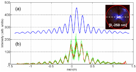
Figure 5: Intensity crosscuts along $k_{x}$ of the image shown in Fig. 4 (f) [see also inset, where the white dashed line indicates the crosscut direction while the actual tip coordinates $[x,y]$ are indicated in brackets]. (a): Theoretical modeling deliberately shifted in the intensity direction for clarity. (b): The green curves shown correspond to several crosscuts and the red curve gives their average.

confirmed experimentally as shown in Fig. 4 for the 3 different diameters $D$. The tip is approximately located at the center of the ring cavity and the simulation are realized with the full Eq. 11. The good agreement between experiments (Figs. 4(d), 4(e), 4(c)) and our model (Figs. 4(g), 4(h), 4(i)) demonstrates the validity of our semi-analytical description. We point out that the vertical dipole STM tip would lead to completely different images. As an example, the numerical calculation for the STM tip placed at the center of the corral is shown in the inset of Fig. 4 (i). It indeed reveals a vortex like structure with topological charge $\pm 1$ in clear disagreement with the experiment (Fig. 4(f)). A better agreement is even obtained if we consider the actual position of the tip in Fig. 4(i) which is slightly off the center (by an amount of 250 nm) along the x axis. This is shown in Fig. 5 where crosscuts were taken along, and parallel (i.e. very close) to, the $k_{x}$ axis of the intensity mapped in Fig. 4(i). The average intensity obtained is in good agreement with the theoretical predictions of our model. In this context it is also interesting to calculate the scattered field in the Fourier space with the hypothesis that the circular slit responds as a distribution of vertical dipoles instead of in-plane dipoles, whereas the NSOM tip still behaves like an in-plane dipole. In analogy with the discussion preceding Eq. 10, we get here:

$$\textbf{E}(\mathbf{k}_{||})\simeq\textrm{const.}\frac{2i\pi\sqrt{2}e^{ik_{\textrm{SP}}D/2}}{\sqrt{D}}$$

$$J_{1}(k_{||}D/2)(\hat{\mathbf{k}}_{||}\cdot\hat{\mathbf{p}}_{||})\hat{\mathbf{k}}_{||}\frac{\sin{\theta}}{\sqrt{\cos{\theta}}}$$ (15)

If we drop the smooth $\sin{\theta}$ variation, this result is intermediate between Eq. 14 and 13 since it combines a vortex of topological charge $\pm 1$ with a cos like pattern (i.e. the term $(\hat{\mathbf{k}}_{||}\cdot\hat{\mathbf{p}}_{||})$). Such behavior is clearly excluded by the data shown in Figs. 4 and 5.

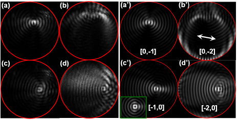
Figure 6: SP excitation of two subwavelength apertures by a ex-centered NSOM tip. (a-d) correspond to the experimental Fourier space images while (a’-d’) are the associated theoretical images. The white arrow indicates the tip polarization and the brackets indicate the $[x,y]$ tip coordinates.

All this analysis therefore confirms that in the considered case (Figs. 4 and 5) the circular slit acts locally as a sort of Malus polarizer for the in-plane SP electric field.
As a final analysis it is relevant to study further the Fourier space images when the NSOM tip is not located at the center of the circular cavity. This is shown in Fig. 6 for a $D=5$ $\mu$m diameter cavity and for the tip displaced along the x or y axis respectively by an amount of approximately 1 or 2 $\mu$m (i.e., still inside the cavity). The data of Fig. 6(a-d) are compared in Fig. 6(a’-d’) with the theoretical model using Eq. 11. Again, a good agreement is recovered despite some differences at large angles

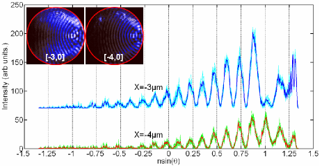
Figure 7: Intensity crosscuts along $k_{x}$ of the images shown in the inset. The white dashed line indicates the crosscut direction and the actual coordinate $[x,y]$ of the tip are indicated in brackets. Crosscuts corresponding to $x=-3$ and $-4$ $\mu$m have be shifted along the intensity axis for clarity.

attributed to either optical misalignments or to some NSOM tip asymmetries. The most interesting feature is the observation of SP fringes of typical periodicity $\delta k=2\pi/D$ observed in Fig. 6(d) (and recovered in the simulation of Fig. 6 (d’)) when the tip is displaced along the x axis. These fringes are absent if the tip is displaced along the y axis. This is explained by the fact that the tip polarisation is mainly oriented along the x axis. Therefore, SPs couple favorably to the slit parts intersecting the x axis and practically do not couple along the y axis. The system actually acts like a Young double slit or hole experiment in strong analogy with what was obtained in refs. Gan ; Kuzmin and particularly ref. sample . However, in contrast with the double hole experiment, here the light sources are spatially extended and curved so that a simple analysis identical to what was done in Section 3 and in ref. sample is not possible. Still, we show in Fig. 7 Fourier space images obtained when the NSOM tip is now outside the ring cavity i.e. displaced by an amount of 3 of 4 $\mu$m along the x axis. Crosscuts made along the $k_{x}$ axis in the Fourier space show first that the fringe periodicity $\delta(n\sin{\theta})=\lambda/D\simeq 0.13$ obtained in the double-slit experiment is indeed recovered. Second, we observe that the fringe minimum and maximum do not move when we go from the case where the NSOM tip is located at $x=-3$ $\mu$m to the position $x=-4$ $\mu$m. This is explained by the fact that the phase shift between the two parts of the slit contributing to the Fourier space image (i.e., those parts of the slit intersecting the x axis) is given in magnitude by $kn_{\textrm{SP}}|R_{1}-R_{2}|$, where $R_{1}$ and $R_{2}$ are respectively the distance between the tip and the part of the slit located at $x\simeq D/2$ and $x\simeq-D/2$ (see Eq. 9). Since $R_{1}-R_{2}=D$ when the tip is outside the cavity this phase shift is the same in the two cases considered and no fringe displacement is expected. This is also in qualitative agreement with the model which reproduces this main feature.

V Conclusion

In this article we have developed a semi-analytical approach able to analyze plasmonic interferometry using scanning near-field SP sources of two kinds: STM and NSOM tips. Our method, mainly based on a scalar Debye-Green formalism for electric and magnetic dipole sources with proper consideration of the propagation through the collection objective, was specifically adapted to describe recent experiments using a STM source in a Young double hole experiment. The model clearly reproduces the observed features sample and predicts some interesting configuration which could be used in the future to probe the aperture dipole directionality. We also focused our attention, both experimentally and theoretically, on plasmonic interferometry on a circular slit achieved with a NSOM source. The measurements were successfully compared to our model, thereby proving the efficiency of our approach. We expect this work to have important applications in the field of plasmonics where optical vortices and manipulation of the light polarization are coupled to near-field microscopy [11,46-48].

Acknowledgements: We thank Jean-François Motte, from NANOFAB facility in Neel Institute for the optical tip manufacturing and FIB milling of the circular slits used in this work. This work was supported by Agence Nationale de la Recherche (ANR), France, through the PLASTIPS, SINPHONIE and PLACORE projects.

References

- (1) W. L. Barnes, A. Dereux, and T. W. Ebbesen, Nature 424, 824 (2003).
- (2) A. Drezet, et al. Mat. Sci. Eng. B 149, 220-229 (2008).
- (3) L. Novotny, The History of Near-field Optics, Progress in Optics 50, E. Wolf (ed.), chapter 5, p.137-184 (Elsevier, Amsterdam The Netherlands, 1997).
- (4) O. Marti, et al. Optics. Commun. 96, 225-228 (1993).
- (5) P. Dawson, F. de Fornel, J.-P. Goudonnnet, Phys. Rev. Lett, 72, 2927-2930 (1994).
- (6) S. I. Bozhevolnyi, Phys. Rev. B 54, 8177 8185 (1996).
- (7) J.R Krenn, R. Wolf , A. Leitner, F.R Aussenegg, Optics. Commun. 137, 46-40 (1997).
- (8) H. Ditlbacher, et al., Phys. Rev. Lett. 95, 257403 (2005).
- (9) Z. Liu, et al. Nano Lett. 5, 1726-1729 (2005).
- (10) Y. Babayan, et al. ACS Nano 3, 615-620 (2009).
- (11) Y. Gorodetski, A. Niv, V. Kleiner, and E. Hasman, Phys. Rev. Lett 101, 043903 (2008)
- (12) B. Hecht, H. Bielefeldt, L. Novotny, Y. Inouye, and D. W. Pohl, Phys. Rev. Lett. 77, 1889-1892 (1996).
- (13) L. Novotny, B. Hecht and D. Pohl, J. Appl. Phys. 81, 1798-1806 (1997).
- (14) F. I. Baida, D. Van Labeke, A. Bouhelier, T. Huser, D. Pohl, J. Opt. Soc. Am. A 18, 1552-1561 (2001).
- (15) A. Bouhelier, Th. Huser, H. Tamaru, H.-J. Güntherodt, and D. W. Pohl, Phys. Rev. B 63, 155404 (2001).
- (16) C. Sönnichsen, A. C. Duch, G. Steininger, M. Koch, G. von Plessen, and J. Feldmann, Appl. Phys. Lett. 76, 140-143 (2000).
- (17) M. Brun, A. Drezet, H. Mariette, N. Chevalier, J. C. Woehl, and S. Huant, Europhys. Lett. 64, 634-640 (2003).
- (18) A. Cuche, et al., Opt. Express 17, 19969-19980 (2009).
- (19) A. Drezet, A. Cuche, and S. Huant, Opt. Commun. 284, 1444-1450 (2011).
- (20) A. Cuche, O. Mollet, A. Drezet, and S. Huant, Nano Lett. 10, 4566-4570 (2010).
- (21) O. Mollet, et al., Phys. Rev. B 86, 045401 (2012).
- (22) O. Mollet, S. Huant, and A. Drezet, Opt. Express 20, 28923-28928 (2012).
- (23) C. Obermüller, K. Karrai, G. Kolb, G. Abstreiter, Ultramicroscopy 61,171-177 (1995).
- (24) A. Drezet, J. C. Woehl and S. Huant, Europhys. Lett. 54, 736-740 (2001).
- (25) A. Drezet, M. J. Nasse, S. Huant and J. C. Woehl, Europhys. Lett. 66, 41-47 (2004).
- (26) T. J. Antosiewicz, T. Szoplik, Opt. Express 15 7845-7852 (2007).
- (27) A. N. Sommerfeld, Ann. Phys. 333, 665-736 (1909).
- (28) A. Yu Nikitin, F. J. García-Vidal, and L. Martín-Moreno, Phys. Rev. Lett. 105, 073902 (2010).
- (29) A. Drezet, C. Genet, Phys. Rev. Lett. 110, 213901 (2013).
- (30) A. Hohenau, J. R. Krenn, A. Drezet, O. Mollet, S. Huant, C. Genet, B. Stein, and T. W. Ebbesen, Opt. Express 19, 25749-25762 (2011).
- (31) P. Bharadwaj, A. Bouhelier, and L. Novotny, Phys. Rev. Lett. 106, 226802 (2011).
- (32) T. Wang, E. Boer-Duchemin, Y. Zhang, G. Comtet, and G. Dujardin, Nanotechnology 22, 175201 (2011).
- (33) J.K. Gimzewski, J.K. Sass, R.R. Schlitter, J. Schott, Europhys. Lett. 8, 435-440 (1989).
- (34) R. Berndt, J.K. Gimzewski, P. Johansson, Phys. Rev. Lett. 67, 3796-3799 (1991).
- (35) R. Marty, C. Girard, A. Arbouet, G. Colas des Francs, Chem Phys. Lett. 532, 100-105 (2012).
- (36) G. Colas des Francs, et al., Phys. Rev. Lett. 86, 4950-4953 (2001).
- (37) C. Chicane, et al., Phys. Rev. Lett. 88, 097402 (2002).
- (38) R. Marty, A. Arbouet, V. Paillard, C. Girard, and G. Colas des Francs, Phys. Rev. B 82, 081403 (2010).
- (39) M. Specht, J. D. Pedarnig, W. M. Heckl, and T. W. Hänsch, Phys. Rev. Lett. 68, 476-479 (1992).
- (40) N. Rotenberg, et al., Phys. Rev. Lett. 108, 127402 (2012).
- (41) L. Yin, et al., Appl. Phys. Lett. 85, 467-469 (2004).
- (42) Y. Zhang,et al., Opt. Express 21, 13938-13948 (2013)
- (43) C. H. Gan, G. Gbur, and T. D. Visser, Phys. Rev. Lett. 98, 043908 (2007).
- (44) N. Kuzmin, et al., Opt. Lett. 32,445-447 (2007).
- (45) J.-M. Yi, A. Cuche, F. de León-Pérez, et al. Phys. Rev. Lett. 109, 023901 (2012).
- (46) E. Lombard, A. Drezet, C. Genet and T. W. Ebbesen, New J. Phys 12, 023027 (2010).
- (47) A. Drezet, C. Genet and T. W. Ebbesen, Phys. Rev. Lett. 101, 043902 (2008).
- (48) Y. Gorodetski, A. Drezet, C. Genet,and T. W. Ebbesen, Phys. Rev. Lett. 110, 203906 (2013).
- (49) P.B. Johnson, R.W. Christy, Phys. Rev. B 6 4370-4379 (1972) .
- (50) H. Bethe, Phys. Rev. 66, 163-182 (1944).
- (51) C. J Bouwkamp, Rep. Prog. Phys 17, 35-100, (1950).
- (52) A. Roberts, J. Opt. Soc. Am. A 4, 1970-1983 (1987).
- (53) E. Popov, et al., J. Opt. Soc. Am. A 24, 339-358 (2007).
- (54) H. W. Kihm, et al., Nature Commun. 2, 451 (2011).
- (55) W. T. Tang, E. Chung, Y.-H. Kim, P. T. C. So, and C. J. R. Sheppard, Opt. Express 15, 4634-4646 (2007).
- (56) M. U. González, et al., Phys. Rev. B 73, 155416 (2006)
- (57) A. Degiron, H. J. Lezec, N. Yamamoto, T.W. Ebbesen, Opt. Commun. 239, 61-65 (2004).