Supplementary for “Imaging surface plasmons: the fingerprint of leaky waves on the far field”

I introduction

We start with a scalar potentials expansion of the electromagnetic field in the three media $j=1,2,3$ corresponding respectively to air metal and substrate (i.e. glass or fused silica). There is no source in the substrate and the dipole (point source) is located in medium $j=1$. We write for the field in each medium:

$$\mathbf{D}_{j}=\boldsymbol{\nabla}\times\boldsymbol{\nabla}\times[\mathbf{\hat{z}}\Psi_{\textrm{TM},j}]+ik_{0}\varepsilon_{j}\boldsymbol{\nabla}\times[\mathbf{\hat{z}}\Psi_{\textrm{TE},j}]$$

$$\mathbf{B}_{j}=\boldsymbol{\nabla}\times\boldsymbol{\nabla}\times[\mathbf{\hat{z}}\Psi_{\textrm{TE},j}]-ik_{0}\boldsymbol{\nabla}\times[\mathbf{\hat{z}}\Psi_{\textrm{TM},j}]$$ (1)

with

$$[\boldsymbol{\nabla}^{2}+k_{0}^{2}\varepsilon_{j}]\Psi_{\textrm{TM,TE},j}=0.$$ (2)

Using Boundary conditions we show that the only non vanishing scalar potentials for the dipole direction perpendicular to the film is in medium $j=3$

$$\Psi^{\textrm{TM},\bot}(\mathbf{x},z)=\frac{i\mu_{\bot}}{4\pi}\int_{0}^{+\infty}\frac{kdk}{k_{1}}\tilde{T}_{13}^{\textrm{TM}}(k)e^{ik_{1}h}e^{ik_{3}z}J_{0}(k\varrho)$$

$$=\frac{i\mu_{\bot}}{8\pi}\int_{-\infty}^{+\infty}\frac{kdk}{k_{1}}\tilde{T}_{13}^{\textrm{TM}}(k)e^{ik_{1}h}e^{ik_{3}z}H_{0}^{(+)}(k\varrho),$$ (3)

where we defined $k_{i}=\sqrt{k_{0}^{2}\varepsilon_{i}-k^{2}}$ with $\textrm{Imag}[k_{j}]\geq 0$, $k_{0}=2\pi/\lambda=\omega/c$, and $z\geq d$. To obtain Eq. 3 we also used the formula $H^{(+)}_{0}(u)-H^{(+)}_{0}(-u)=2J_{0}(u)$ which is valid in the complex plane $u=u^{\prime}+iu^{\prime\prime}$ (if $|\arg{(z)}|<\pi$). The Fresnel coefficient characterizing the transmission of the metal film is for TM waves defined by

$$\tilde{T}_{13}^{\textrm{TM}}(k)=\frac{T_{23}^{\textrm{TM}}T_{12}^{\textrm{TM}}}{1+R_{23}^{\textrm{TM}}R_{12}^{\textrm{TM}}e^{2ik_{2}d}}e^{i(k_{2}-k_{3})d}$$ (4)

where

$$R_{ij}^{\textrm{TM}}=\frac{k_{i}/\varepsilon_{i}-k_{j}/\varepsilon_{j}}{k_{i}/\varepsilon_{i}+k_{j}/\varepsilon_{j}}$$ (5)

$$T_{ij}^{\textrm{TM}}=\frac{2k_{i}/\varepsilon_{i}}{k_{i}/\varepsilon_{i}+k_{j}/\varepsilon_{j}}.$$ (6)

We then introduce the variables $k=k_{0}n\sin{\xi}$, $k_{3}=k_{0}n\cos{\xi}$ with $\xi=\xi^{\prime}+i\xi^{\prime\prime}$ and write

$$\Psi^{\textrm{TM},\bot}(\mathbf{x},z)=\int_{\Gamma}d\xi F_{+}^{\textrm{TM},\bot}(\xi)e^{ik_{0}n((z-d)\cos{\xi}+\varrho\sin{\xi})}$$ (7)

with

$$F_{+}^{\textrm{TM},\bot}(\xi)=\frac{i\mu_{\bot}}{8\pi}\frac{k_{0}n\sin{\xi}\cos{\xi}}{\sqrt{(\frac{\varepsilon_{1}}{\varepsilon_{3}}-\sin^{2}{\xi})}}\tilde{T}_{13}^{\textrm{TM}}(k_{0}n\sin{\xi})$$

$$e^{i\sqrt{(\frac{\varepsilon_{1}}{\varepsilon_{3}}-\sin^{2}{\xi})}h}\cdot e^{ik_{0}nd\cos{\xi}}H_{0}^{(+)}(k_{0}n\varrho\sin{\xi})e^{-ik_{0}n\varrho\sin{\xi}}$$

(we point out that the $\varrho$ and $\varphi$ dependencies are here and in the following implicit in our notation: $F_{+}(\xi):=F_{+}(\xi,\varphi,\varrho)$). Similar expressions can be obtained for the components $\boldsymbol{\mu}_{||}$ of the dipole parallel to the interface. More precisely for the TM modes we have

$$\Psi^{\textrm{TM},||}(\mathbf{x},z)=\int_{\Gamma}d\xi F_{+}^{\textrm{TM},||}(\xi)e^{ik_{0}n((z-d)\cos{\xi}+\varrho\sin{\xi})}$$ (9)

with

$$F_{+}^{\textrm{TM},||}(\xi)=\frac{\boldsymbol{\mu}_{||}\cdot\hat{\boldsymbol{\varrho}}}{8\pi}k_{0}n\cos{\xi}\tilde{T}_{13}^{\textrm{TM}}(k_{0}n\sin{\xi})$$

$$e^{i\sqrt{(\frac{\varepsilon_{1}}{\varepsilon_{3}}-\sin^{2}{\xi})}h}\cdot e^{ik_{0}nd\cos{\xi}}H_{1}^{(+)}(k_{0}n\varrho\sin{\xi})e^{-ik_{0}n\varrho\sin{\xi}}.$$

Similarly for the TE waves we obtain:

$$\Psi^{\textrm{TE},||}(\mathbf{x},z)=\int_{\Gamma}d\xi F_{+}^{\textrm{TE},||}(\xi)e^{ik_{0}n((z-d)\cos{\xi}+\varrho\sin{\xi})}$$ (11)

with

$$F_{+}^{\textrm{TE},||}(\xi)=-\frac{\boldsymbol{\mu}_{||}\cdot\hat{\boldsymbol{\varphi}}}{8\pi}\frac{k_{0}\cos{\xi}}{\sqrt{(\frac{\varepsilon_{1}}{\varepsilon_{3}}-\sin^{2}{\xi})}}\tilde{T}_{13}^{\textrm{TE}}(k_{0}n\sin{\xi})$$

$$e^{i\sqrt{(\frac{\varepsilon_{1}}{\varepsilon_{3}}-\sin^{2}{\xi})}h}\cdot e^{ik_{0}nd\cos{\xi}}H_{1}^{(+)}(k_{0}n\varrho\sin{\xi})e^{-ik_{0}n\varrho\sin{\xi}}.$$

We used the formula $H^{(+)}_{1}(u)+H^{(+)}_{1}(-u)=2J_{1}(u)$. Here the Fresnel coefficients are defined by

$$\tilde{T}_{13}^{\textrm{TE}}(k)=\frac{T_{23}^{\textrm{TE}}T_{12}^{\textrm{TE}}}{1+R_{23}^{\textrm{TE}}R_{12}^{\textrm{TE}}e^{2ik_{2}d}}e^{i(k_{2}-k_{3})d}$$ (13)

with

$$R_{ij}^{\textrm{TE}}=\frac{k_{i}-k_{j}}{k_{i}+k_{j}}$$ (14)

$$T_{ij}^{\textrm{TE}}=\frac{2k_{i}}{k_{i}+k_{j}}.$$ (15)

The presence of the singular Hankel functions $H_{1}^{(+)}$ and $H_{0}^{(+)}$ in all these expressions imply the existence of a branch cut starting at the origin and associated with the function $1/\sqrt{(\sin{\xi})}$. This branch cut is chosen in order to have no influence during subsequent contour deformations and is running just below the actual path $\Gamma$ slightly off the real axis $\xi^{\prime}$ and to the left of the vertical line $\xi^{\prime\prime}=-\pi/2$ (the original branch cut is composed of the line $\xi^{\prime}=-\pi/2$ and of the half-axis [$\xi^{\prime\prime}=0$, $\xi^{\prime}\leq 0$]). We also introduce the polar coordinates $\varrho=r\sin{\vartheta}$, $z=d+r\cos{\vartheta}$ leading to $(z-d)\cos{\xi}+\varrho\sin{\xi}=r\cos{(\xi-\vartheta)}$ and therefore:

$$\Psi(\mathbf{x},z)=\int_{\Gamma}d\xi F_{+}(\xi)e^{ik_{0}nr\cos{(\xi-\vartheta)}}.$$ (16)

The definition of the square root $k_{1}=k_{0}n\sqrt{(\frac{\varepsilon_{1}}{\varepsilon_{3}}-\sin^{2}{\xi})}$, with $\varepsilon_{3}=n^{2}$ real and $\varepsilon_{1}=\varepsilon_{1}^{\prime}+i\varepsilon_{1}^{\prime\prime}\sim 1+i\delta$ with $\delta\rightarrow 0^{+}$, implies the presence of a branch cut which must be chosen carefully in order i) to be consistent with the choice for $k_{1}$ made in Eq. 3 during integration along the contour $\Gamma$, ii) to allow further contour deformations leading to convergent calculations. The branch cut adapted to our problem is shown in Figs. 1,2 and correspond to the choice $\textrm{Imag}[k_{1}]\geq 0$ in the whole complex $\xi$-plane. The branch cut starts at the branch point $M$ of coordinate $\xi_{c}$ defined by the condition $k_{1}=0$. We point out that due to invariance of the Fresnel coefficient $\tilde{T}_{13}^{\textrm{TM},\textrm{TE}}(k_{0}n\sin{\xi})$ over the permutation $k_{2}\leftrightarrow-k_{2}$ we don’t actually need an additional branch cut for $k_{2}$ (this important property will survive for a larger number of layers).

II The different contributions along the closed contour

After introducing the function $f(\xi)=i\cos(\xi-\vartheta)=i\cos{(\xi^{\prime}-\vartheta)}\cosh{\xi^{\prime\prime}}+\sin{(\xi^{\prime}-\vartheta)}\sinh{\xi^{\prime\prime}}$ we define the steepest descent path $SDP$ by the condition

$$\textrm{Imag}[f(\xi)]=\cos{(\xi^{\prime}-\vartheta)}\cosh{\xi^{\prime\prime}}=1.~{}$$ (17)

$SDP$ goes through the saddle point $\xi_{0}$ defined by the condition $\frac{df(\xi)}{d\xi}=0$ which has a solution at $\xi_{0}=\vartheta$. Importantly, there are actually two trajectories solutions of Eq. 17 and going through $\xi_{0}$. We choose the one such that the real part of $f(\xi)$ decay uniformly along $SDP$ when going away arbitrarily to the left or to the right from the saddle point(see Fig. 1).
Cauchy theorem allows us to deform the original $\Gamma$ contour to include $SDP$ as a part of the integration path. For this we label $\Gamma$ by the letter $ABCD$ (see Fig. 1). The integral in Eq. 16 is thus written $\int_{\Gamma}=\int_{ABCD}$. We will consider two cases depending whether $\vartheta$ is or not larger than the real part of the branch point $\xi^{\prime}_{c}\simeq\arcsin{(1/n)}=\vartheta_{c}$.

II.1 Closing the contour in the case $\vartheta>\xi^{\prime}_{c}$

If $\vartheta>\xi^{\prime}_{c}$ the closed integration contour contain eight contributions (see Fig. 1) and we have:

$$0=\int_{\Gamma}+\int_{DE}+\int_{EF}+\tilde{\int_{FG}}+\tilde{\int_{GH}}+\int_{HI}+\int_{IA}-I_{SP}.$$ (18)

The contribution

$$\int_{DE}:=\int_{DE}d\xi F_{+}(\xi)e^{ik_{0}nr\cos{(\xi-\vartheta)}}$$

$$=\int_{\pi/2-i\infty}^{\pi/2+\vartheta-i\infty}d\xi F_{+}(\xi)e^{ik_{0}nr\cos{(\xi-\vartheta)}}$$ (19)

approaches zero asymptotically and can therefore be neglected.
Similarly, we can neglect $\int_{IA}:=\int_{+i\infty}^{-\pi/2+i\infty}d\xi F_{+}(\xi)e^{ik_{0}nr\cos{(\xi-\vartheta)}}$ which approaches also zero asymptotically.
The contribution $\int_{EF}$ and $\tilde{\int_{FG}}$ are calculated along the $SDP$. However, due to the presence of the branch cut crossing $SDP$ at $F$ the integration along $FG$ actually corresponds to a change of Riemann sheet associated with the second determination for the square root $k_{1}$ (we point out that since the branch cut is very close to the imaginary axis at $F$ we have at the limit $\xi_{F}\simeq i\textrm{arccosh}{(1/\cos{\vartheta})}$). More precisely if we call “+” the Riemann sheet in which $\textrm{Imag}[k_{1}]\geq 0$ the second Riemann

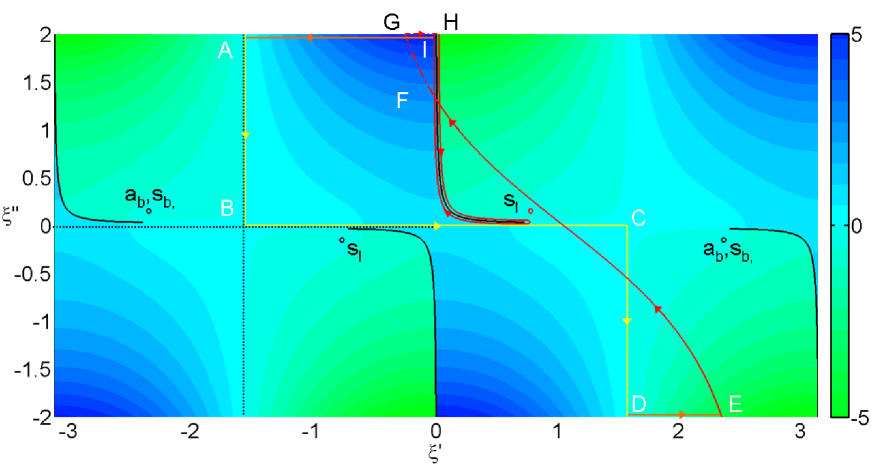
Figure 1: Integration contour in the complex $\xi$-plane for $\vartheta>\xi^{\prime}_{c}$.

surface “-” associated with the condition $\textrm{Imag}[k_{1}]\leq 0$ is connected to “+” through the branch cut represented in Fig. 1. Therefore, crossing the branch cut at $F$ corresponds actually to a change in sign of the square root $k_{1}\rightarrow-k_{1}$. We have consequently the contributions

$$\int_{EF}:=\int_{EF}d\xi F_{+}(\xi)e^{ik_{0}nr\cos{(\xi-\vartheta)}}$$

$$\tilde{\int_{FG}}:=\int_{FG}d\xi F_{-}(\xi)e^{ik_{0}nr\cos{(\xi-\vartheta)}}$$ (20)

where $F_{-}(\xi)$ is the same function of $k$ as $F_{+}(\xi)$ but $\sqrt{(\frac{\varepsilon_{1}}{\varepsilon_{3}}-\sin^{2}{\xi})}$ (defined with $\textrm{Imag}[\sqrt{(\frac{\varepsilon_{1}}{\varepsilon_{3}}-\sin^{2}{\xi})}]\geq 0$) is now replaced by $-\sqrt{(\frac{\varepsilon_{1}}{\varepsilon_{3}}-\sin^{2}{\xi})}$. More precisely the square root $z_{+}=\sqrt{g}$ of the complex variable $g^{\prime}+ig^{\prime\prime}$ is defined on the “+” Riemann sheet by $z_{+}=\textrm{sign}(g^{\prime\prime})\sqrt{((g^{\prime}+|g|)/2)}+i\sqrt{((-g^{\prime}+|g|)/2)}$ where $\textrm{sign}(x)=1$ if $x>0$, $\textrm{sign}(x)=-1$ if $x<0$ and $\textrm{sign}(x)=0$ if $x=0$. On the“-” sheet we have therefore $z_{-}=-z_{+}$. An important remark concerns here the integration convergence along the SDP when approaching the vertical asymptotes $\pm\frac{\pi}{2}+\vartheta\mp i\infty$. Indeed, due to the presence of the coefficient $e^{\pm ik_{0}nh\sqrt{(\frac{\varepsilon_{1}}{\varepsilon_{3}}-\sin^{2}{\xi})}}$ in the definition of $F_{\pm}(\xi)$ it is not obvious that the integrand will take a finite value at infinity. Actually a careful study of the limit behaviour of $F_{\pm}(\xi)$ including the exponentials terms as well as the Hankel function contribution shows that there is no convergence problem for $F_{+}(\xi)$ at infinity (this also explains why $\int_{DE}$ and $\int_{IA}$ goes to zero asymptotically). However when going on the “-” Riemann sheet the convergence is not always ensured. We found that however no problem occurs on this second sheet as soon as the condition $z+\varrho\tan{\vartheta}>h$ is verified. In particular, no problem appears if we impose $z>h$. Since here we are interested in the asymptotic behavior valid for $z\gg h$ this condition will be automatically satisfied.
This point is particularly relevant when we consider the contribution $\tilde{\int}_{GH}:=\int_{-\pi/2+\vartheta+i\infty}^{i\infty}d\xi F_{-}(\xi)e^{ik_{0}nr\cos{(\xi-\vartheta)}}$ which approaches zero if the previous condition $z>h$ is fulfilled. From $H$ we thus cross the branch cut and go back to the “+” sheet. We thus obtain a contour $\int_{HI}=\int_{HI}d\xi F_{+}(\xi)e^{ik_{0}nr\cos{(\xi-\vartheta)}}$ longing the branch cut in the original “+” space and contourning the branch point $k_{1}=0$ (corresponding nearly to $\xi_{c}\simeq\arcsin{(1/n)}=\vartheta_{c}$). We will see in the subsection D that this contribution corresponds to a lateral wave associated with a Goos-Hänchen effect in transmission.
Finally, due to the presence of isolated singularities in the complex plane (i.e. poles) for the TM waves we must subtract a residue contribution $I_{SP}$ which value will precisely depends on the position $\vartheta$ along the real axis (i.e. whether or not the poles are encircled by the closed contour in the complex $\xi$-plane). A complete analysis of these singularities show that we can in principle extract from the transmission coefficient $\tilde{T}_{13}^{\textrm{TM}}(k)$ four poles corresponding to the four SP modes guided along the metal slab. However, the branch cut choice made here allows only the existence of three solutions called respectively symmetric leaky ($s_{l}$), symmetric bound ($s_{b}$) and asymmetric bound ($a_{b}$) modes. The two bound modes are always well outside the region of integration and are never encircled by the contour. Only the leaky mode $s_{l}$ can eventually contribute as a residue depending whether or not the angle $\vartheta$ is larger than the leakage radiation angle $\vartheta_{LR}$ defined by the condition $\cos{(\xi_{p}^{\prime}-\vartheta_{LR})}\cosh{\xi_{p}^{\prime\prime}}=1$ (with $\xi_{p}$ the complex coordinate of the SP pole $s_{l}$). This implies:

$$\vartheta_{LR}=\xi_{p}^{\prime}+\arccos{(1/\cosh{\xi_{p}^{\prime\prime}})}\simeq\xi_{p}^{\prime},$$ (21)

and therefore the residue contribution is written:

$$I_{SP}=2\pi i\textrm{Res}[F_{+}(\xi_{p})]e^{ik_{0}nr\cos{(\xi_{p}-\vartheta)}}\Theta(\vartheta-\vartheta_{LR}).$$

In the following we write $k_{p}=k_{0}n\sin{\xi_{p}}$, $k_{3,p}=k_{0}n\cos{\xi_{p}}$ and $k_{1,p}=k_{0}n\sqrt{(\frac{\varepsilon_{1}}{\varepsilon_{3}}-\sin^{2}{\xi_{p}})}$ the pole wavevectors associated with this $s_{l}$ mode. The calculation of the different residues is straightforward and leads for the vertical dipole case to:

$$\textrm{Res}[F_{+}^{\textrm{TM},\bot}(\xi_{p})]e^{ik_{0}nr\cos{(\xi_{p}-\vartheta)}}=\frac{i\mu_{\bot}}{8\pi}\frac{k_{0}n\sin{\xi_{p}}\cos{\xi_{p}}}{\sqrt{(\frac{\varepsilon_{1}}{\varepsilon_{3}}-\sin^{2}{\xi_{p}})}}\textrm{Res}[\tilde{T}_{13}^{\textrm{TM}}(k_{0}n\sin{\xi_{p}})]e^{i\sqrt{(\frac{\varepsilon_{1}}{\varepsilon_{3}}-\sin^{2}{\xi_{p}})}h}\cdot e^{ik_{0}nz\cos{\xi_{p}}}H_{0}^{(+)}(k_{0}n\varrho\sin{\xi_{p}})$$

We now write $\tilde{T}_{13}^{\textrm{TM}}(k)$ as a rational fraction $\frac{N_{13}(k)}{D_{13}(k)}$ (with polynomial functions $N_{13}(k)$, $D_{13}(k)$ of the variable $k$) and therefore for the single pole $\xi_{p}$ we get

$$\textrm{Res}[\tilde{T}_{13}^{\textrm{TM}}(k_{0}n\sin{\xi_{p}})]=\frac{N_{13}(k_{p})}{\frac{\partial D_{13}(k_{0}n\sin{\xi_{p}})}{\partial\xi_{p}}}=\frac{1}{k_{3,p}}\frac{N_{13}(k_{p})}{\frac{\partial D_{13}(k_{p})}{\partial k_{p}}}.$$

We thus have finally

$$\textrm{Res}[F_{+}^{\textrm{TM},\bot}(\xi_{p})]e^{ik_{0}nr\cos{(\xi_{p}-\vartheta)}}$$

$$=\frac{i\mu_{\bot}}{8\pi}\frac{k_{p}}{k_{1,p}}e^{ik_{1,p}h}e^{ik_{3,p}z}\frac{N_{13}(k_{p})}{\frac{\partial D_{13}(k_{p})}{\partial k_{p}}}H_{0}^{(+)}(k_{p}\varrho).$$ (24)

A similar expression is obtained for the horizontal dipole:

$$\textrm{Res}[F_{+}^{\textrm{TM},||}(\xi_{p})]e^{ik_{0}nr\cos{(\xi_{p}-\vartheta)}}$$

$$=\frac{\boldsymbol{\mu}_{||}\cdot\hat{\boldsymbol{\varrho}}}{8\pi}e^{ik_{1,p}h}e^{ik_{3,p}z}\frac{N_{13}(k_{p})}{\frac{\partial D_{13}(k_{p})}{\partial k_{p}}}H_{1}^{(+)}(k_{p}\varrho).$$ (25)

There is no residue for the TE modes.
Going back to the SDP contribution we define the variable $\tau=e^{i\pi/4}\sqrt{2}\sin{((\xi-\vartheta)/2)}$ which leads to $f(\xi)=i-\tau^{2}$. Along $SDP$ $\tau$ is real such that $\tau^{2}=-\sin{(\xi^{\prime}-\vartheta)}\sinh{\xi^{\prime\prime}}\geq 0$. We thus obtain $\tau=2\sin{((\xi^{\prime}-\vartheta)/2)}\cosh{(\xi^{\prime\prime}/2)}$. The saddle point corresponds to $\tau=0$ ($\tau>0$ if $\xi^{\prime\prime}<0$ and $\tau<0$ if $\xi^{\prime\prime}>0$ along $SDP$). With this new variable the point $F$ has therefore the coordinate $\tau_{F}\simeq-2\sin{(\vartheta/2)}\cosh{(\frac{1}{2}\textrm{arccosh}(1/\cos(\vartheta)))}=-2\sin{(\vartheta/2)}\sqrt{1+\frac{1}{\cos{\vartheta}}}<0$. Defining the term $I_{SDP}=-\int_{EF}-\tilde{\int_{FG}}$ we therefore obtain

$$I_{SDP}=e^{ik_{0}nr}\{\int_{-\infty}^{\tau_{F}^{-}}d\tau G_{-}(\tau)e^{-k_{0}nr\tau^{2}}$$

$$+\int_{\tau_{F}^{+}}^{+\infty}d\tau G_{+}(\tau)e^{-k_{0}nr\tau^{2}}\}$$

$$=e^{ik_{0}nr}\int_{-\infty}^{+\infty}d\tau\{G_{+}(\tau)[1-\Theta(\tau_{F}-\tau)]$$

$$+G_{-}(\tau)[1-\Theta(\tau-\tau_{F})]\}e^{-k_{0}nr\tau^{2}}$$ (26)

where we defined $G_{\pm}(\tau)=F_{\pm}(\xi)\frac{d\xi}{d\tau}$ and used $\frac{d\xi}{d\tau}=\sqrt{2}e^{-i\pi/4}/\cos{((\xi-\vartheta)/2)}$. We introduced the Heaviside step function $\Theta(x)$ defined as: $\Theta(x)=1$ if $x\geq 0$ and $\Theta(x)=0$ otherwise. Importantly $\lim_{\tau\rightarrow\tau_{F}^{+}}G_{+}(\tau)=\lim_{\tau\rightarrow\tau_{F}^{-}}G_{-}(\tau)$ and therefore the function $G(\tau)=G_{+}(\tau)(1-\Theta(\tau_{F}-\tau))+G_{-}(\tau)(1-\Theta(\tau-\tau_{F}))$ which is not defined at $\tau_{F}$ can be prolonged without difficulties at $F$.

II.2 Closing the contour in the case $\vartheta<\xi^{\prime}_{c}$

If $\vartheta<\xi^{\prime}_{c}$ the closed integration contour contain 6 contributions (see Fig. 2) and we have:

$$0=\int_{\Gamma}+\int_{DE}+\int_{EF}+\tilde{\int_{FG}}+\int_{GH}+\int_{HA}.$$ (27)

All these contribution but $\int_{NM}$ are defined on the “+” Riemann sheet. $\int_{HA}$ and $\int_{DE}$ tends asymptotically to zero for reasons already discussed in the previous

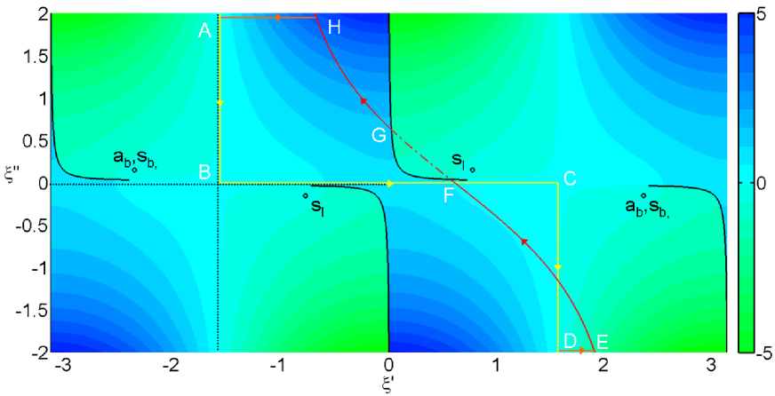
Figure 2: Integration contour in the complex $\xi$-plane for $\vartheta<\xi^{\prime}_{c}$.

paragraph. Importantly there is no contribution along the branch cut since the integration path along SDP starts and finishes on the proper Riemann sheet “+”. Regrouping the terms we thus have for $\vartheta>\xi^{\prime}_{c}$: $\int_{\Gamma}=I_{SDP}=-\int_{EF}-\tilde{\int_{FG}}-\int_{GH}$ with

$$\int_{EF}:=\int_{EF}d\xi F_{+}(\xi)e^{ik_{0}nr\cos{(\xi-\vartheta)}}$$

$$\tilde{\int_{FG}}:=\int_{FG}d\xi F_{-}(\xi)e^{ik_{0}nr\cos{(\xi-\vartheta)}}$$

$$\int_{GH}:=\int_{GH}d\xi F_{+}(\xi)e^{ik_{0}nr\cos{(\xi-\vartheta)}}.$$ (28)

We then use the same variable $\tau$ and function $G_{\pm}(\tau)$ and thus obtain

$$I_{SDP}=e^{ik_{0}nr}\{\int_{-\infty}^{\tau_{F}^{-}}d\tau G_{+}(\tau)e^{-k_{0}nr\tau^{2}}$$

$$+\int_{\tau_{F}^{+}}^{\tau_{G}^{-}}d\tau G_{+}(\tau)e^{-k_{0}nr\tau^{2}}$$

$$+\int_{\tau_{G}^{+}}^{-\infty}d\tau G_{+}(\tau)e^{-k_{0}nr\tau^{2}}\}$$ (29)

which is rewritten as

$$I_{SDP}=e^{ik_{0}nr}\int_{-\infty}^{\tau_{F}^{-}}d\tau G(\tau)e^{-k_{0}nr\tau^{2}}$$ (30)

with

$$G(s)=G_{+}(\tau)[1-\Theta(\tau-\tau_{F})]$$

$$+G_{+}(\tau)[1-\Theta(\tau_{G}-\tau)]$$

$$+G_{-}(\tau)[1-\Theta(\tau_{F}-\tau)][1-\Theta(\tau-\tau_{G})].$$ (31)

II.3 The Steepest descent path contribution

The previous integral $I_{SDP}$ for both $\vartheta>\xi^{\prime}_{c}$ and $\vartheta<\xi^{\prime}_{c}$ is of the gaussian form and can be evaluated by doing a Taylor expansion of $G(\tau)$ around $\tau=0$. Using well known integrals we thus obtain

$$I_{SDP}=e^{ik_{0}nr}\sum_{m\in\textrm{even}}\frac{\Gamma(\frac{m+1}{2})}{m!(k_{0}nr)^{\frac{m+1}{2}}}\frac{d^{m}}{d\tau^{m}}G(0).$$ (32)

It is important to observe that $G(\tau)$ is highly singular in the vicinity of the SP pole $s_{l}$. Writing $\tau_{p}$ the coordinate of the pole in the $\tau$-space we thus define

$$G(\tau):=G_{0}(\tau)+\frac{\textrm{Res}[G(\tau_{p})]}{\tau-\tau_{p}}$$ (33)

which (together with Eq. 32) immediately implies

$$I_{SDP}=e^{ik_{0}nr}\sum_{m\in\textrm{even}}\frac{\Gamma(\frac{m+1}{2})}{(k_{0}nr)^{\frac{m+1}{2}}}\{\frac{1}{m!}\frac{d^{m}}{d\tau^{m}}G_{0}(0)$$

$$-\frac{\textrm{Res}[G(\tau_{p})]}{\tau_{p}^{m+1}}\}.$$ (34)

Remarkably, the singular integral

$$I_{SDP}^{\textrm{pole}}:=e^{ik_{0}nr}\int_{-\infty}^{+\infty}d\tau\frac{\textrm{Res}[G(\tau_{p})]}{\tau-\tau_{p}}e^{-k_{0}nr\tau^{2}}$$

can be directly calculated and we thus obtain

$$I_{SDP}=e^{ik_{0}nr}\sum_{m\in\textrm{even}}\frac{\Gamma(\frac{m+1}{2})}{m!(k_{0}nr)^{\frac{m+1}{2}}}\frac{d^{m}}{d\tau^{m}}G_{0}(0)+I_{SDP}^{\textrm{pole}}$$

with

$$I_{SDP}^{\textrm{pole}}=-2i\pi\textrm{Res}[G(\tau_{p})]e^{ik_{0}nr\cos{(\xi_{p}-\vartheta)}}\{\Theta(-\tau_{p}^{\prime\prime})$$

$$-\frac{1}{2}\textrm{erfc}(-i\tau_{p}\sqrt{(k_{0}nr)})\}$$

$$=-e^{ik_{0}nr}\sum_{m\in\textrm{even}}\frac{\Gamma(\frac{m+1}{2})}{(k_{0}nr)^{\frac{m+1}{2}}}\frac{\textrm{Res}[G(\tau_{p})]}{\tau_{p}^{m+1}}$$ (36)

where $\textrm{erfc}(z)=(2/\sqrt{\pi})\int_{z}^{+\infty}e^{-t^{2}}dt$ is the Gauss complementary error function. Notably, we have (see appendix) $\textrm{Res}[G(\tau_{p})]=\textrm{Res}[F_{+}(\xi_{p})]$ and $\Theta(-\tau_{p}^{\prime\prime})=\Theta(\vartheta-\vartheta_{LR})$ therefore $I_{SDP}^{\textrm{pole}}$ contains up to the sign difference the same contribution which already appeared in $I_{SP}$. Consequently, the sum $I_{SDP}^{\textrm{pole}}+I_{SP}$ of the two contributions proportional to the residue represents a simple explicit mathematical expression:

$$I_{SDP}^{\textrm{pole}}+I_{SP}$$

$$=i\pi\textrm{Res}[G(\tau_{p})]e^{ik_{0}nr\cos{(\xi_{p}-\vartheta)}}\textrm{erfc}(-i\tau_{p}\sqrt{(k_{0}nr)}).$$ (37)

This sum is sometimes by definition associated with the surface plasmon mode. We point out however that the error function is highly singular and therefore we should preferably use the equivalent expression:

$$I_{SDP}^{\textrm{pole}}+I_{SP}=2i\pi\textrm{Res}[G(\tau_{p})]e^{ik_{0}nr\cos{(\xi_{p}-\vartheta)}}\Theta(\vartheta-\vartheta_{LR})$$

$$-e^{ik_{0}nr}\sum_{m\in\textrm{even}}\frac{\Gamma(\frac{m+1}{2})}{(k_{0}nr)^{\frac{m+1}{2}}}\frac{\textrm{Res}[G(\tau_{p})]}{\tau_{p}^{m+1}}.$$

We also note that most of the discussions and confusions made during the XX^th on the role of SPs in the Sommerfeld integral resulted from the above mentioned intricate relationship existing between the two singular terms $I_{SP}$ and $I_{SDP}^{\textrm{pole}}$. For a historical discussion see CollinCollin .

II.4 The lateral wave contribution: Goos-Hänchen effect in transmission

In the case $\vartheta>\xi^{\prime}_{c}$ the integral $\int_{HI}$ along the branch cut can be transformed using the method described in Ref. 2. For this we separate the integral $\int_{HI}d\xi F_{+}(\xi)e^{ik_{0}nr\cos{(\xi-\vartheta)}}$ into

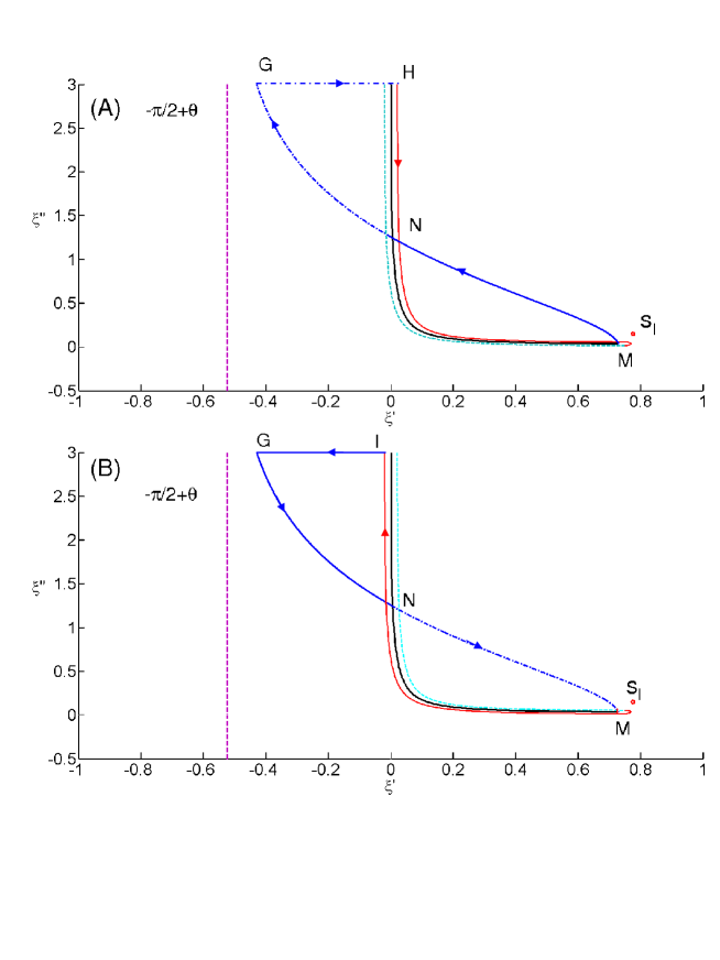
Figure 3: Integration contour in the complex $\xi$-plane along the branch cut $HI$ around the branch point $M$ for $\vartheta>\xi^{\prime}_{c}$. (A) shows the closed contour used to deform analytically the contour $HM$. (B) shows the closed contour used to deform the contour $MI$.

a contribution $\int_{HM}=\int_{HM}d\xi F_{+}(\xi)e^{ik_{0}nr\cos{(\xi-\vartheta)}}$ starting at infinity at $\xi=i\infty+0^{+}$ and stopping at the branch-point $M$ ($\xi_{c}\simeq\vartheta_{c}$) and into a contribution $\int_{MI}=\int_{MI}d\xi F_{+}(\xi)e^{ik_{0}nr\cos{(\xi-\vartheta)}}$ starting at $M$ and finishing at infinity $\xi=i\infty+0^{-}$ on the other side of the branch cut. As shown in Fig. 3(A) in order to calculate $I_{HM}$ the integration contour is closed by longing the modified steepest descent path $MG$ defined by the equation

$$\cos{(\xi^{\prime}-\vartheta)}\cosh{\xi^{\prime\prime}}=\cos{(\xi_{c}^{\prime}-\vartheta)}\cosh{\xi_{c}^{\prime\prime}}$$

$$\simeq\cos{(\vartheta_{c}-\vartheta)}=K<1.$$ (39)

The curve $MG$ with a vertical asymptote at $\xi=-\pi/2+\vartheta$ is thus defined by $\xi^{\prime\prime}=\textrm{arccosh}(K/\cos{(\xi^{\prime}-\vartheta)})$. We thus have $0=\int_{HM}+\int_{MN}+\tilde{\int}_{NG}+\tilde{\int}_{GH}$ where $N$ is the intersection point between the modified steepest descent path $MG$ and the branch cut ($\xi_{N}\simeq i\textrm{arccosh}(K/\cos{(\vartheta)})$). $\tilde{\int}_{NG}:=\int_{NG}d\xi F_{-}(\xi)e^{ik_{0}nr\cos{(\xi-\vartheta)}}$ and $\tilde{\int}_{GH}:=\int_{GH}d\xi F_{-}(\xi)e^{ik_{0}nr\cos{(\xi-\vartheta)}}$ are evaluated on the “-” Riemann sheet while $\int_{HM}:=\int_{HM}d\xi F_{+}(\xi)e^{ik_{0}nr\cos{(\xi-\vartheta)}}$ and $\int_{MN}:=\int_{MN}d\xi F_{+}(\xi)e^{ik_{0}nr\cos{(\xi-\vartheta)}}$ are evaluated on the “+” Riemann sheet. From $H$ we cross a second time the branch cut in order to close the contour on the “+” Riemann sheet.
A similar analysis is done for the integration contour $\int_{MI}$. We have $0=\int_{MI}+\int_{IG}+\int_{GN}+\tilde{\int}_{NM}$ where $\int_{MI}$, $\int_{IG}$ and $\int_{GN}$ are defined as previously on the “+” Riemann sheet while $\tilde{\int}_{NM}:=\int_{NM}d\xi F_{-}(\xi)e^{ik_{0}nr\cos{(\xi-\vartheta)}}$ is evaluated on the “-” Riemann sheet. In order to close the contour in “+” we must finally cross the branch cut in the region surrounding $M$. The infinitesimal loop surrounding $M$ gives however a vanishing contribution which can be neglected.
Regrouping all these expressions we define $I_{LW}=-\int_{HM}-\int_{MI}$ and we obtain

$$I_{LW}=\int_{\xi_{c}}^{\xi_{N}}d\xi[F_{+}(\xi)-F_{+}(\xi)]e^{ik_{0}nr\cos{(\xi-\vartheta)}}+\int_{\xi_{N}}^{-\pi/2+\vartheta+i\infty}d\xi[F_{-}(\xi)-F_{+}(\xi)]e^{ik_{0}nr\cos{(\xi-\vartheta)}}+\int_{IG}+\tilde{\int_{GH}}.$$ (40)

The contributions $\int_{IG}$, $\tilde{\int_{GH}}$ vanish asymptotically as discussed before and therefore can be neglected. Importantly due to the definition of the square root the function $F_{-}(\xi)-F_{+}(\xi)$ tends to vanish at the intersection point $N$. We then define the function $\Phi(\xi)=[F_{+}(\xi)-F_{+}(\xi)]\textrm{sign}(\xi^{\prime\prime}_{N}-\xi^{\prime\prime})$ vanishing at $\xi_{c}$ and write

$$I_{LW}=\Theta(\vartheta-\xi^{\prime}_{c})\int_{\xi_{c}}^{-\pi/2+\vartheta+i\infty}d\xi\Phi(\xi)e^{ik_{0}nr\cos{(\xi-\vartheta)}}.$$

The Heaviside function was introduced in order to remember that $I_{LW}$ is only defined if $\xi^{\prime}_{c}<\vartheta$. In the present work we will only evaluate $I_{LW}$ approximately using the method discussed in Ref. 2. First, we observe that $e^{ik_{0}nr\cos{(\xi-\vartheta)}}=e^{ik_{0}nrK}e^{k_{0}nr\sin{(\xi^{\prime}-\vartheta)}\sinh{\xi^{\prime\prime}}}$. Second, considering that only $\xi$ values in the vicinity of $\xi_{c}\simeq\vartheta_{c}$ contribute significantly to $I_{LW}$ we write $d\xi\approx id\xi^{\prime\prime}$, and $\sin{(\xi^{\prime}-\vartheta)}\sinh{\xi^{\prime\prime}}\approx-\sin{(\vartheta-\vartheta_{c})}\xi^{\prime\prime}<0$. We therefore obtain

$$I_{LW}\approx ie^{ik_{0}nrK}\Theta(\vartheta-\vartheta_{c})\int_{0}^{+\infty}d\xi^{\prime\prime}\Phi(\vartheta_{c}+i\xi^{\prime\prime})e^{-k_{0}nr\sin{(\vartheta-\vartheta_{c})}\xi^{\prime\prime}}$$

$$=2ie^{ik_{0}nrK}\Theta(\vartheta-\vartheta_{c})\int_{0}^{+\infty}udu\Phi(\vartheta_{c}+iu^{2})e^{-k_{0}nr\sin{(\vartheta-\vartheta_{c})}u^{2}}$$ (42)

where we used the variable $\xi^{\prime\prime}=u^{2}$. This integral is of the Gaussian kind and can be computed exactly using a Taylor expansion of $\Phi$ near $\vartheta_{c}$. We consequently deduce

$$I_{LW}\approx ie^{ik_{0}nrK}\Theta(\vartheta-\vartheta_{c})\sum_{m=1}^{+\infty}\frac{\Gamma(1+m/2)}{(k_{0}nr\sin{(\vartheta-\vartheta_{c})})^{1+m/2}}\frac{H^{(m)}(0)}{m!}$$ (43)

where we used the series expansion $\Phi(\vartheta_{c}+iu^{2})=H(u)=\sum_{m=1}^{+\infty}\frac{u^{m}}{m!}\frac{d^{m}}{du^{m}}H(u)|_{u=0}=\sum_{m=1}^{+\infty}u^{m}\frac{H^{(m)}(0)}{m!}$ (the term $m=0$ vanishes since $\Phi(\theta_{c})=0$).

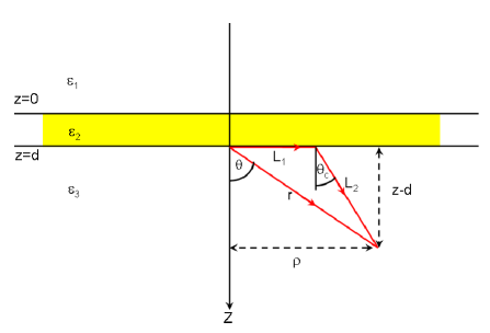
Figure 4: Geometric construction of the Goos-Hänchen phase in transmission.

The phase $\delta\varphi=k_{0}nr\cos{(\vartheta-\vartheta_{c})}=k_{0}nr[\cos{\vartheta}\cos{\vartheta_{c}}+\sin{\vartheta}\sin{\vartheta_{c}}]$ takes a simple interpretation if you define the length $L_{1}$ of $L_{2}$ by:

$$r\sin{\vartheta}=\varrho=L_{1}+L_{2}\sin{\vartheta_{c}}$$

$$r\cos{\vartheta}=z-d=L_{2}\cos{\vartheta_{c}}.$$ (44)

Therefore we obtain

$$\delta\varphi=k_{0}n(L_{2}+L_{1}\sin{\vartheta_{c}})=k_{0}nL_{2}+k_{0}L_{1}$$ (45)

where we used $n\sin{\vartheta_{c}}=1$. As it is clear from Fig. 4 $L_{1}$ is the path length of a ‘creeping’ wave propagating along the interface before to be re-emitted at the critical angle $\vartheta_{c}$. The re-emitted waves propagates along a distance $L_{2}$ in the medium of optical index $n$ and then reaches the point defined by the coordinates $(r,\vartheta)$. The phase $\delta\varphi$ is thus generated by a virtual propagation of length $L_{1}$ along the interface air-dielectric $z=d$ (supposing no metal is present and that the volume corresponding to the film between $z=0$ and $z=d$ is filled with the medium of permittivity $\varepsilon_{1}\simeq 1$) and followed by a re-emission at the critical angle in the glass substrate $\varepsilon_{3}=n^{2}$. The previous analysis justifies therefore the name “lateral” we gave to the contribution $I_{LW}$. This effect can be seen as a kind of Goos-Hänchen deflection in transmission and is somehow equivalent to the already known Goos-Hänchen effect associated with lateral waves in the reflection mode.

II.5 The Far-field Fraunhofer regime

We are interested into evaluating the different integrals when $r\rightarrow+\infty$. As a first approximation, concerning $I_{SDP}$ we calculate only the term $m=0$ in the sum which reads:

$$I_{SDP,m=0}=\frac{\sqrt{\pi}e^{ik_{0}nr}}{\sqrt{k_{0}nr}}G(0)=\frac{\sqrt{2\pi}e^{ik_{0}nr}e^{-i\pi/4}}{\sqrt{k_{0}nr}}F_{+}(\vartheta).$$ (46)

In the far-field where $r>>\lambda$ the Hankel function can be approximated using the asymptotic formulas

$$H^{(+)}_{0}(x)=\sqrt{\frac{2}{\pi x}}e^{-i\pi/4}(1-\frac{i}{8x})e^{ix}+O(x^{-5/2})$$

$$H^{(+)}_{1}(x)=\sqrt{\frac{2}{\pi x}}e^{-i3\pi/4}(1+\frac{3i}{8x})e^{ix}+O(x^{-5/2})$$ (47)

which are valid for $x>>1$. Therefore for the vertical dipole we get

$$I_{SDP,m=0}^{\bot}=\frac{2\pi k_{0}n\cos{\vartheta}}{ir}e^{ik_{0}nr}\tilde{\Psi}^{\textrm{TM},\bot}[k_{0}n\sin{\vartheta}\boldsymbol{\hat{\varrho}},z=d(1-\frac{i}{8k_{0}nr\sin{\vartheta}^{2}}+...)$$ (48)

where

$$\tilde{\Psi}_{\textrm{TM},\bot}[\mathbf{k},z=d]=\frac{i\mu_{\bot}}{8\pi^{2}k_{1}}\tilde{T}_{13}^{\textrm{TM}}(k)e^{ik_{3}d}e^{ik_{1}h}$$

$$=\frac{i\mu_{\bot}}{8\pi^{2}k_{0}\sqrt{(1-n^{2}\sin{\vartheta}^{2})}}\tilde{T}_{13}^{\textrm{TM}}(k)e^{ik_{3}d}e^{ik_{1}h}$$ (49)

is the 2D Fourier transform of $\Psi^{\textrm{TM},\bot}(\varrho,z)$ calculated at $z=d$ (i.e $\int\frac{d^{2}\mathbf{x}}{4\pi^{2}}\Psi^{\textrm{TM},\bot}(\varrho,z=d)e^{-i\mathbf{k}\cdot\mathbf{x}}$) for the wavevector $\mathbf{k}=k_{0}n\sin{\vartheta}\boldsymbol{\hat{\varrho}}$. Similarly for the Horizontal dipole we obtain for TM components:

$$I_{SDP,m=0}^{||}=\frac{2\pi k_{0}n\cos{\vartheta}}{ir}e^{ik_{0}nr}\tilde{\Psi}^{\textrm{TM},||}[k_{0}n\sin{\vartheta}\boldsymbol{\hat{\varrho}},z=d](1+\frac{3i}{8k_{0}nr\sin{\vartheta}^{2}}+...)$$ (50)

where

$$\tilde{\Psi}^{\textrm{TM},||}[\mathbf{k},z=d]=\frac{-i\mu_{||}\cdot\mathbf{k}}{8\pi^{2}k^{2}}\tilde{T}_{13}^{\textrm{TM}}(k)e^{ik_{3}d}e^{ik_{1}h}$$

$$=\frac{-i\mu_{||}\cdot\boldsymbol{\hat{\varrho}}}{8\pi^{2}k_{0}nr\sin{\vartheta}}\tilde{T}_{13}^{\textrm{TM}}(k)e^{ik_{3}d}e^{ik_{1}h}.$$ (51)

For TE components we have also:

$$I_{SDP,m=0}^{||}=\frac{2\pi k_{0}n\cos{\vartheta}}{ir}e^{ik_{0}nr}\tilde{\Psi}^{\textrm{TE},||}[k_{0}n\sin{\vartheta}\boldsymbol{\hat{\varrho}},z=d](1+\frac{3i}{8k_{0}nr\sin{\vartheta}^{2}}+...)$$ (52)

with now

$$\tilde{\Psi}^{\textrm{TE},||}[\mathbf{k},z=d]=\frac{ik_{0}\mu_{||}\cdot(\mathbf{\hat{z}}\times\mathbf{k})}{8\pi^{2}k_{1}k^{2}}\tilde{T}_{13}^{\textrm{TE}}(k)e^{ik_{3}d}e^{ik_{1}h}$$

$$=\frac{i\mu_{||}\boldsymbol{\hat{\varphi}}}{8\pi^{2}k_{0}\sqrt{(1-n^{2}\sin{\vartheta}^{2})}n\sin{\vartheta}}\tilde{T}_{13}^{\textrm{TE}}(k)e^{ik_{3}d}e^{ik_{1}h}.$$ (53)

In the far field only the term in $1/r$ survives and (in agreement with the Stratton-Chu formalism stratton and Richards and Wolf wolf ) we can always write:

$$\Psi\simeq I_{SDP,m=0}\simeq\frac{2\pi k_{0}n\cos{\vartheta}}{ir}e^{ik_{0}nr}$$

$$\tilde{\Psi}^{\textrm{TM or te}}[k_{0}n\sin{\vartheta}\boldsymbol{\hat{\varrho}},z=d].$$ (54)

II.6 The intermediate regime: Generalization of the Norton wave

The next term in the power expansion of $\Psi$ contributes proportionally to $1/r^{2}$. To evaluate this term we must take into account not only $I_{SDP,m=0}$ but also $I_{SDP,m=2}$ and $I_{LW,m=1}$. We use the notation

$$F_{\pm}(\xi)=\sqrt{(\frac{2\pi k_{0}n}{r})}e^{-i\frac{\pi}{4}}k_{0}n\cos{\xi}Q_{\pm}^{\alpha}(k_{0}n\sin{\xi})$$

$$\cdot[1-i\frac{1-4\alpha^{2}}{k_{0}nr(\sin{\xi})^{2}}+...]$$ (55)

(with $\alpha=0$ or 1 depending whether the dipole is vertical or horizontal) and we obtain for the SDP contributions proportional to $1/r^{2}$:

$$I_{SDP,m=0}=\frac{2\pi(1-4\alpha^{2})}{r^{2}}e^{ik_{0}nr}\frac{\cos{\vartheta}Q_{+}^{\alpha}(k_{0}n\sin{\xi})}{(\sin{\vartheta})^{2}}$$ (56)

and

$$I_{SDP,m=2}=\frac{e^{ik_{0}nr}\sqrt{\pi}}{4(k_{0}nr)^{3/2}}\frac{d^{2}G(\tau)}{d\tau^{2}}|_{\tau=0}$$

$$=\frac{-\pi}{r^{2}}e^{ik_{0}nr}\frac{d^{2}[\frac{\cos{\xi}}{\cos{((\xi-\vartheta)/2)}}Q_{+}^{\alpha}(k_{0}n\sin{\xi})]}{d\xi^{2}}|_{\xi=\vartheta}.$$

We also have to include the lateral wave (i.e. Goos-Hänchen) contribution:

$$I_{LW,m=1}\simeq e^{ik_{0}nrK}\frac{i\sqrt{\pi}\Theta(\vartheta-\vartheta_{c})}{2(k_{0}nr\sin{(\vartheta-\vartheta_{c})})^{3/2}}\frac{dH(u)}{du}|_{u=0}$$ (58)

which reads

$$I_{LW,m=1}=\frac{\pi e^{ik_{0}(nL_{2}+L_{1})}\Theta(\vartheta-\vartheta_{c})e^{i\frac{\pi}{4}}}{r^{2}(\sin{(\vartheta-\vartheta_{c})})^{3/2}}\frac{d\{\cos(\vartheta_{c}+iu^{2})[Q_{+}^{\alpha}(k_{0}n\sin{(\vartheta_{c}+iu^{2})})-Q_{-}^{\alpha}(k_{0}n\sin{(\vartheta_{c}+iu^{2})})]\}}{du}|_{u=0}.$$ (59)

The sum $I_{SDP,m=0}+I_{SDP,m=2}+I_{LW,m=1}$ describes an asymptotic field varying as $1/r^{2}$ and which constitutes a generalization of the result obtained by Norton for the radio wave antenna on a conducting earth problem.

III How to define the surface plasmon mode?

III.1 From the near-field to the far-field

As seen in Section 2.E the dominant contribution in the far-field has the form

$$\Psi(\mathbf{x},z)=\frac{2\pi k_{0}n\cos{\vartheta}}{ir}e^{ik_{0}nr}\tilde{\Psi}[k_{0}n\sin{\vartheta}\boldsymbol{\hat{\varrho}},z=d].$$ (60)

From Eq. 53 we also have the relation

$$\tilde{\Psi}[k_{0}n\sin{\vartheta}\boldsymbol{\hat{\varrho}},z=d]:=Q(s)$$

$$=\sqrt{(\frac{r}{2\pi k_{0}n})}e^{i\frac{\pi}{4}}\frac{F_{+}(\xi)}{k_{0}n\cos{\xi}}$$

$$=\sqrt{(\frac{r}{2\pi k_{0}n})}e^{i\frac{\pi}{4}}F_{+}(\xi)\frac{d\xi}{ds}$$ (61)

where $s=k_{0}n\sin{\xi}$ and where $\xi$ is here identical to $\vartheta$ (as usual the $\varrho$ and $\varphi$ dependencies are here implicit in $Q(s):=Q(s,\varphi,\varrho)$ and $F_{+}(\xi):=F_{+}(\xi,\varphi,\varrho)$). In the complex plane $\xi=\xi^{\prime}+i\xi^{\prime\prime}$ and $s=s^{\prime}+is^{\prime\prime}$ we have the singular/regular decomposition: $Q(s)=Q_{0}(s)+\textrm{Res}[Q(s_{p})]/(s-s_{p})$. Furthermore, from Eq. 59 this implies

$$\frac{1}{2\pi i}\oint_{C_{p}}dsQ(s)=\textrm{Res}[Q(s_{p})]$$

$$=\sqrt{(\frac{r}{2\pi k_{0}n})}e^{i\frac{\pi}{4}}\frac{1}{2\pi i}\oint_{\mathcal{C}_{p}}d\xi F_{+}(\xi)$$

$$=\sqrt{(\frac{r}{2\pi k_{0}n})}e^{i\frac{\pi}{4}}\textrm{Res}[F_{+}(\xi_{p})]$$ (62)

where $C_{p}$ and $\mathcal{C}_{p}$ are small closed contours surrounding the plasmon pole in respectively the complex $s$-plane and $\xi$-plane. Therefore, we can equivalently write

$$Q(s)=Q_{0}(s)+\sqrt{(\frac{r}{2\pi k_{0}n})}e^{i\frac{\pi}{4}}\frac{\textrm{Res}[F_{+}(\xi_{p})]}{s-s_{p}}.$$ (63)

The calculations being done in the far-field limit, where $r,\varrho\rightarrow+\infty$, we have for the vertical dipole case the residue:

$$\textrm{Res}[F_{+}^{\textrm{TM},\bot}(\xi_{p})]=\frac{i\mu_{\bot}}{8\pi}\frac{k_{p}}{k_{1,p}}e^{ik_{1,p}h}e^{ik_{3,p}d}\frac{N_{13}(k_{p})}{\frac{\partial D_{13}(k_{p})}{\partial k_{p}}}H_{0}^{(+)}(k_{p}\varrho)e^{-ik_{p}\varrho}\simeq\frac{i\mu_{\bot}}{8\pi}\frac{k_{p}}{k_{1,p}}e^{ik_{1,p}h}e^{ik_{3,p}d}\frac{N_{13}(k_{p})}{\frac{\partial D_{13}(k_{p})}{\partial k_{p}}}\sqrt{(\frac{2}{\pi k_{p}\varrho})}e^{-i\frac{\pi}{4}},2$$ (64)

and similarly for the horizontal dipole residue:

$$\textrm{Res}[F_{+}^{\textrm{TM},||}(\xi_{p})]=\frac{\boldsymbol{\mu}_{||}\cdot\hat{\boldsymbol{\varrho}}}{8\pi}e^{ik_{1,p}h}e^{ik_{3,p}d}\frac{N_{13}(k_{p})}{\frac{\partial D_{13}(k_{p})}{\partial k_{p}}}H_{1}^{(+)}(k_{p}\varrho)e^{-ik_{p}\varrho}\simeq\frac{\boldsymbol{\mu}_{||}\cdot\hat{\boldsymbol{\varrho}}}{8\pi}e^{ik_{1,p}h}e^{ik_{3,p}d}\frac{N_{13}(k_{p})}{\frac{\partial D_{13}(k_{p})}{\partial k_{p}}}\sqrt{(\frac{2}{\pi k_{p}\varrho})}e^{-i\frac{3\pi}{4}}.$$ (65)

Regrouping all the terms and using the fact that $Q(s)=\tilde{\Psi}[\mathbf{k},z=d]$ with $\mathbf{k}=k_{0}n\sin{\vartheta}\boldsymbol{\hat{\varrho}}$ and $\varrho=r\sin{\vartheta}$ this allow us to obtain a decomposition of the Fourier field $\tilde{\Psi}[\mathbf{k},z=d]$ into a singular (i.e. SP) and regular contribution:

$$\tilde{\Psi}^{\bot,||}[\mathbf{k},z=d]=\tilde{\Psi}^{\bot,||}_{0}[\mathbf{k},z=d]+\tilde{\Psi}^{\bot,||}_{SP}[\mathbf{k},z=d]$$ (66)

with

$$\tilde{\Psi}^{\bot}_{SP}[\mathbf{k},z=d]=\frac{i\mu_{\bot}}{8\pi}\frac{k_{p}}{k_{1,p}}\frac{e^{ik_{1,p}h}e^{ik_{3,p}d}}{\pi\sqrt{kk_{p}}(k-k_{p})}\frac{N_{13}(k_{p})}{\frac{\partial D_{13}(k_{p})}{\partial k_{p}}}$$

$$\tilde{\Psi}^{||}_{SP}[\mathbf{k},z=d]=\frac{\boldsymbol{\mu}_{||}\cdot\hat{\mathbf{k}}}{8\pi}\frac{e^{ik_{1,p}h}e^{ik_{3,p}d}}{i\pi\sqrt{kk_{p}}(k-k_{p})}\frac{N_{13}(k_{p})}{\frac{\partial D_{13}(k_{p})}{\partial k_{p}}}.$$ (67)

These formulas are rigorously only valid in the propagative sector where $|\mathbf{k}|\leq k_{0}n$ (i.e. from the far-field definition). However, due to the simplicity of the mathematical expressions obtained one is free to extend the validity of Eqs. 65 to the full spectrum of $\mathbf{k}\in\mathbb{R}^{2}$ values including both the propagative sector for which $k_{3}=\sqrt{(k_{0}^{2}n^{2}-|\mathbf{k}|^{2})}$ and the evanescent sector for which $k_{3}=i\sqrt{(|\mathbf{k}|^{2}-k_{0}^{2}n^{2})}$ (i.e. if $|\mathbf{k}|\geq k_{0}n$).
It should now be observed that we can slightly modify our current analysis by observing that Eq. 61 is not exactly a Laurent series since there are other isolated singularities in the complex plane which were here included in the definition of $Q_{0}(s)$ i.e. $\tilde{\Psi}^{\bot,||}_{0}[\mathbf{k},z=d]$. The previous choice was justified for all practical purposes by the detailed calculation done in Section 2 in which only the $\xi_{p}$ singularity corresponding to the $s_{l}$ mode contributed to the integration contours used. Still, for the symmetry of the mathematical expressions it is clearly possible, and actually very useful (as we will see below), to extract a second SP contribution $\xi_{-p}=-\xi_{p}$ corresponding to $-k_{p}$. This is clearly the $s_{l}$ pole associated with propagation in the opposite radial direction. Taking into account this second pole and the symmetries of $k_{1p}$, $k_{3p}$, $N_{13}(k_{p})$ and antisymmetry of $\frac{\partial D_{13}(k_{p})}{\partial k_{p}}$ in the substitution $k_{p}\rightarrow-k_{p}$ one obtain after straightforward calculations:

$$\tilde{\Psi}^{\bot}_{SP}[\mathbf{k},z=d]:=\frac{i\mu_{\bot}}{8\pi}\frac{k_{p}}{k_{1,p}}\frac{e^{ik_{1,p}h}e^{ik_{3,p}d}}{\pi\sqrt{k_{p}}}\frac{N_{13}(k_{p})}{\frac{\partial D_{13}(k_{p})}{\partial k_{p}}}\frac{1}{\sqrt{k}}[\frac{1}{k-k_{p}}+\frac{1}{i(k+k_{p})}]$$

$$\tilde{\Psi}^{||}_{SP}[\mathbf{k},z=d]:=\frac{\boldsymbol{\mu}_{||}\cdot\hat{\mathbf{k}}}{8\pi}\frac{e^{ik_{1,p}h}e^{ik_{3,p}d}}{\pi\sqrt{k_{p}}}\frac{N_{13}(k_{p})}{\frac{\partial D_{13}(k_{p})}{\partial k_{p}}}\frac{1}{\sqrt{k}}[\frac{1}{i(k-k_{p})}+\frac{1}{k+k_{p}}].$$ (68)

From this definition we can calculate the SP field in the complete space. In particular for $z\geq d$ we have $\Psi^{\bot,||}_{SP}(\mathbf{x},z)=\int d^{2}\mathbf{k}\tilde{\Psi}^{\bot,||}_{SP}[\mathbf{k},z=d]e^{ik_{3}Z}$ with $Z=z-d$. More precisely using the symmetry of the system we obtain

$$\Psi^{\bot}_{SP}(\mathbf{x},z)=\frac{i\mu_{\bot}}{8\pi}\frac{k_{p}}{k_{1,p}}\frac{e^{ik_{1,p}h}e^{ik_{3,p}d}}{\pi\sqrt{k_{p}}}\frac{N_{13}(k_{p})}{\frac{\partial D_{13}(k_{p})}{\partial k_{p}}}$$

$$\cdot 2\pi\int_{0}^{+\infty}\frac{kdke^{ik_{3}Z}J_{0}(k\varrho)}{\sqrt{k}}[\frac{1}{k-k_{p}}+\frac{1}{i(k+k_{p})}]$$ (69)

and

$$\Psi^{||}_{SP}(\mathbf{x},z)=\frac{\boldsymbol{\mu}_{||}\cdot\hat{\boldsymbol{\varrho}}}{8\pi}\frac{e^{ik_{1,p}h}e^{ik_{3,p}d}}{\pi\sqrt{k_{p}}}\frac{N_{13}(k_{p})}{\frac{\partial D_{13}(k_{p})}{\partial k_{p}}}$$

$$\cdot 2\pi\int_{0}^{+\infty}\frac{kdke^{ik_{3}Z}J_{1}(k\varrho)}{\sqrt{k}}[\frac{1}{k-k_{p}}-\frac{1}{i(k+k_{p})}].$$ (70)

with $\mathbf{x}=\varrho\hat{\boldsymbol{\varrho}}$. To obtain these last equations we also used the well known Bessel function properties:

$$\oint d\varphi_{k}e^{ik\varrho\cos{(\varphi-\varphi_{k})}}\{\begin{array}[]{c}\cos{(m\varphi_{k})}\\ \sin{(m\varphi_{k})}\end{array}\}$$ (73)

$$=2\pi i^{m}\{\begin{array}[]{c}\cos{(m\varphi)}\\ \sin{(m\varphi)}\end{array}\}J_{m}(k\varrho)$$ (76)

(m=0,1,…) to integrate over the $\varphi_{k}$-coordinate of the 2D vector $\mathbf{k}$.
We point out that the convergence of integrals 69, 70 is ensured since the Cosine integral $\int^{+\infty}_{a}dkcos{(k\varrho)}/k=-\textrm{Ci}(a\varrho)\simeq\frac{\cos{(a\varrho)}}{(a\varrho)^{2}}-\frac{\sin{(a\varrho)}}{a\varrho}$ for $a\varrho\gg 1$ is bounded.

III.2 Asymptotic expansion

Remarkably, using the relations $H^{(+)}_{0}(u)-H^{(+)}_{0}(-u)=2J_{0}(u)$ and $H^{(+)}_{1}(u)+H^{(+)}_{1}(-u)=2J_{1}(u)$ (valid for $|\arg{(z)}|<\pi$) as well as the parity properties of the functions $\frac{1}{\sqrt{k}}[\frac{1}{k-k_{p}}\pm\frac{1}{i(k+k_{p})}]$ (i.e. under the transformation $k_{p}\rightarrow-k_{p}$) we obtain the practical relations

$$\int_{0}^{+\infty}\frac{kdke^{ik_{3}Z}J_{0}(k\varrho)}{\sqrt{k}}[\frac{1}{k-k_{p}}+\frac{1}{i(k+k_{p})}]$$

$$=\frac{1}{2}\int_{-\infty}^{+\infty}\frac{kdke^{ik_{3}Z}H^{(+)}_{0}(k\varrho)}{\sqrt{k}}[\frac{1}{k-k_{p}}+\frac{1}{i(k+k_{p})}]$$ (77)

and

$$\int_{0}^{+\infty}\frac{kdke^{ik_{3}Z}J_{1}(k\varrho)}{\sqrt{k}}[\frac{1}{k-k_{p}}-\frac{1}{i(k+k_{p})}]$$

$$=\frac{1}{2}\int_{-\infty}^{+\infty}\frac{kdke^{ik_{3}Z}H^{(+)}_{1}(k\varrho)}{\sqrt{k}}[\frac{1}{k-k_{p}}-\frac{1}{i(k+k_{p})}].$$ (78)

Those relations would not be possible if we didn’t included both the $k_{p}$ and $-k_{p}$ poles in the analysis. Inserting Eqs. 72,73 into Eqs. 69,70 and using the complex variable $\xi$ such as $k=k_{0}n\sin{\xi}$ and the integration contour $\Gamma$ used in the previous Sections we obtain

$$\Psi^{\bot,||}_{SP}(\mathbf{x},z)=\int_{\Gamma}d\xi F^{\bot,||}_{SP}(\xi)e^{ik_{0}nr\cos{(\xi-\vartheta)}}$$ (79)

where

$$F^{\bot}_{SP}(\xi)=\frac{i\mu_{\bot}}{8\pi}\frac{k_{p}}{k_{1,p}}\frac{\sqrt{(k_{0}n)}e^{ik_{1,p}h}e^{ik_{3,p}d}}{\sqrt{k_{p}}}\frac{N_{13}(k_{p})}{\frac{\partial D_{13}(k_{p})}{\partial k_{p}}}\frac{\sin{\xi}H_{0}^{(+)}(k_{0}n\varrho\sin{\xi})e^{-ik_{0}n\varrho\sin{\xi}}}{\sqrt{\sin{\xi}}}[\frac{\cos{\xi}}{\sin{\xi}-\sin{\xi_{p}}}+\frac{\cos{\xi}}{i(\sin{\xi}+\sin{\xi_{p}})}]$$

$$F^{||}_{SP}(\xi)=\frac{\boldsymbol{\mu}_{||}\cdot\hat{\boldsymbol{\varrho}}}{8\pi}\frac{\sqrt{(k_{0}n)}e^{ik_{1,p}h}e^{ik_{3,p}d}}{\sqrt{k_{p}}}\frac{N_{13}(k_{p})}{\frac{\partial D_{13}(k_{p})}{\partial k_{p}}}\frac{\sin{\xi}H_{1}^{(+)}(k_{0}n\varrho\sin{\xi})e^{-ik_{0}n\varrho\sin{\xi}}}{\sqrt{\sin{\xi}}}[\frac{\cos{\xi}}{\sin{\xi}-\sin{\xi_{p}}}-\frac{\cos{\xi}}{i(\sin{\xi}+\sin{\xi_{p}})}].$$

The integral along $\Gamma$ can be evaluated by using the same contour deformation as in Section 2. However, due to the absence of the square root $k_{1}$ in Eq. 75 there is no branch cut contribution to the integration contour. The integral can thus be split into one contribution from the residue and one contribution from the SDP. We get therefore:

$$\Psi^{\bot,||}_{SP}(\mathbf{x},z)=2\pi i\textrm{Res}[F^{\bot,||}_{SP}(\xi_{p})]e^{ik_{0}nr\cos{(\xi_{p}-\vartheta)}}\Theta(\vartheta-\vartheta_{LR})$$

$$+e^{ik_{0}nr}\sum_{m\in\textrm{even}}\frac{\Gamma(\frac{m+1}{2})}{m!(k_{0}nr)^{\frac{m+1}{2}}}\frac{d^{m}}{d\tau^{m}}G^{\bot,||}_{SP}(0)$$

with $G^{\bot,||}_{SP}(\tau)=F^{\bot,||}_{SP}(\xi)\frac{d\xi}{d\tau}$.
Few remarks are here important:
(i) First, the singular term

$$2\pi i\textrm{Res}[F^{\bot,||}_{SP}(\xi_{p})]e^{ik_{0}nr\cos{(\xi_{p}-\vartheta)}}\Theta(\vartheta-\vartheta_{LR})$$

is exactly identical to the pole contribution appearing in Eq. 22. This results from the equality $\textrm{Res}[F^{\bot,||}_{SP}(\xi_{p})]=\textrm{Res}[F_{+}^{\textrm{TM},\bot,||}(\xi_{p})]$ (compare with Eqs. 24-25).
(ii) Second, the term $m=0$ in the SDP contribution is dominant in the far-field regime and leads to $\Psi^{\bot,||}_{SP}(\mathbf{x},z)=\frac{2\pi k_{0}n\cos{\vartheta}}{ir}e^{ik_{0}nr}\tilde{\Psi}^{\bot,||}_{SP}[k_{0}n\sin{\vartheta}\boldsymbol{\hat{\varrho}},z=d]$ as expected.
(iii) Third, the decomposition $Q(s)=Q_{0}(s)+\textrm{Res}[Q(s_{p})]/(s-s_{p})+\textrm{Res}[Q(-s_{p}]/(s+s_{p})$ leads to

$$G^{\bot,||}_{SP}(\tau)=G^{\bot,||}_{SP,0}(\tau)+\frac{\textrm{Res}[G^{\bot,||}_{SP}(\tau_{p})]}{\tau-\tau_{p}}$$

$$+\frac{\textrm{Res}[G^{\bot,||}_{SP}(\tau_{-p}]}{\tau-\tau_{-p}}$$ (82)

where $\tau_{-p}=-e^{i\pi/4}\sqrt{2}\sin{((\xi_{p}+\vartheta)/2)}$. Therefore, if we compare with Eqs. 32-38 we see that $\Psi^{\bot,||}_{SP}(\mathbf{x},z)$ is not exactly equal to $I_{SP}+I_{SDP}^{\textrm{pole}}$ explicitly defined in Eqs. 37 and 36. More precisely we obtain:

$$\Psi^{\bot,||}_{SP}(\mathbf{x},z)=2i\pi\textrm{Res}[G^{\bot,||}_{SP}(\tau_{p})]e^{ik_{0}nr\cos{(\xi_{p}-\vartheta)}}\Theta(\vartheta-\vartheta_{LR})$$

$$-e^{ik_{0}nr}\sum_{m\in\textrm{even}}\frac{\Gamma(\frac{m+1}{2})}{(k_{0}nr)^{\frac{m+1}{2}}}\frac{\textrm{Res}[G^{\bot,||}_{SP}(\tau_{p})]}{\tau_{p}^{m+1}}$$

$$-e^{ik_{0}nr}\sum_{m\in\textrm{even}}\frac{\Gamma(\frac{m+1}{2})}{(k_{0}nr)^{\frac{m+1}{2}}}\frac{\textrm{Res}[G^{\bot,||}_{SP}(\tau_{-p})]}{\tau_{-p}^{m+1}}$$

$$+e^{ik_{0}nr}\sum_{m\in\textrm{even}}\frac{\Gamma(\frac{m+1}{2})}{m!(k_{0}nr)^{\frac{m+1}{2}}}\frac{d^{m}}{d\tau^{m}}G^{\bot,||}_{SP,0}(0)$$

which differs from Eqs. 37, 38 by the two last lines. We can also rewrite these expressions as

$$\Psi^{\bot,||}_{SP}(\mathbf{x},z)=e^{ik_{0}nr}\sum_{m\in\textrm{even}}\frac{\Gamma(\frac{m+1}{2})}{m!(k_{0}nr)^{\frac{m+1}{2}}}\frac{d^{m}}{d\tau^{m}}G^{\bot,||}_{SP,0}(0)$$

$$+i\pi\textrm{Res}[G^{\bot,||}_{SP}(\tau_{p})]e^{ik_{0}nr\cos{(\xi_{p}-\vartheta)}}\textrm{erfc}(-i\tau_{p}\sqrt{(k_{0}nr)})$$

$$+i\pi\textrm{Res}[G^{\bot,||}_{SP}(\tau_{-p})]e^{ik_{0}nr\cos{(\xi_{p}+\vartheta)}}\textrm{erfc}(-i\tau_{-p}\sqrt{(k_{0}nr)})$$

where we used Eq. 36. applied to $\tau_{-p}$ and $\tau_{p}$.

IV More on intensity and field in the back focal plane and image plane of the microscope

A general analysis of the imaging process occurring through a microscope objective with high numerical aperture $NA$ and an ocular tube lens is given in for example Ref. Sheppard . Here, we give without proofs the calculated field and intensity in the focal plane of the objective and the image plane of the microscope expressed in term of the TE and TM scalar potentials defined in Eqs. 1,2.
For this purpose we use the Fourier transform of the electromagnetic TM and TE field at the $z=d$ interface defined by:

$$\tilde{\mathbf{D}}_{\textrm{TM}}[\mathbf{k},z]=-\{\mathbf{k}k_{3}(k)-k^{2}\hat{\mathbf{z}}\}\tilde{\Psi}_{\textrm{TM}}[\mathbf{k},z]$$

$$\tilde{\mathbf{D}}_{TE}[\mathbf{k},z]=-k_{0}n^{2}\mathbf{k}\times\mathbf{\hat{z}}\tilde{\Psi}_{TE}[\mathbf{k},z].$$ (85)

This implies Sheppard that the electric field recorded in the back focal plane of the objective is (i.e. taking into account the vectorial nature of the field and the transformation of the spherical wave front to a planar wave front):

$$\mathbf{E}_{\textrm{back focal plane $\Pi$}}=\frac{2\pi e^{ik_{0}nf}}{if}\frac{T_{1}\sqrt{k_{0}k_{3}(k)}}{n}\{-k_{0}n\mathbf{k}\tilde{\Psi}_{\textrm{TM}}[\mathbf{k},d]+k_{0}n^{2}k\boldsymbol{\hat{\varphi}}_{1}\tilde{\Psi}_{TE}[\mathbf{k},d]\}$$ (86)

with by definition $\boldsymbol{\hat{\varphi}}_{1}=-\mathbf{k}\times\hat{\mathbf{z}}/k$. The geometric coefficient $k_{3}(k)$ is reminiscent from the ’sin’ condition Sheppard which lead to strong geometrical abberations at very large angle $\theta$. As a direct consequence we deduce the intensity in the back focal plane:

$$|\mathbf{E}_{\textrm{back focal plane $\Pi$}}|^{2}=\frac{4\pi^{2}t_{1}}{f^{2}n^{2}}k_{0}k_{3}(k)[|\mathbf{\tilde{D}}_{\textrm{TM},3}[\mathbf{k},d]|^{2}+|\mathbf{\tilde{D}}_{\textrm{TE},3}[\mathbf{k},d]|^{2}]$$

which is therefore proportional to the total Fourier field intensity for TM and TE waves taken separately.
Finally, in the image plane we obtain the electric field :

$$\mathbf{E}(\mathbf{x}^{\prime})=N^{\prime}\int_{|\mathbf{k}|\leq k_{0}NA}d^{2}\mathbf{k}\sqrt{k_{3}(k)}e^{-i\mathbf{k}\cdot\frac{\mathbf{x}^{\prime}}{M}}\cdot\{\tilde{\mathbf{D}}_{\textrm{TM},||}[\mathbf{k},d]\frac{k_{0}n}{k_{3}(k)}+\tilde{\mathbf{D}}_{\textrm{TE}}[\mathbf{k},d]\}$$

i.e.

$$\mathbf{E}(\mathbf{x}^{\prime})=N^{\prime}\int_{|\mathbf{k}|\leq k_{0}NA}d^{2}\mathbf{k}\sqrt{k_{3}(k)}e^{-i\mathbf{k}\cdot\frac{\mathbf{x}^{\prime}}{M}}\cdot\{-k_{0}n\mathbf{k}\tilde{\Psi}_{\textrm{TM}}[\mathbf{k},d]+k_{0}n^{2}k\boldsymbol{\hat{\varphi}}_{1}\tilde{\Psi}_{\textrm{TE}}[\mathbf{k},d]\}$$ (89)

where $N^{\prime}$ is a constant characterizing the microscope. In the letter we used theses formulas for computing fields and intensity in the Fourier and image plane (see Figs. 3,4 of the letter).

Appendix A

We have by definition

$$\tau_{p}^{\prime\prime}=\sin{((\xi_{p}^{\prime}-\vartheta)/2)}\cosh{(\xi_{p}^{\prime\prime}/2)}$$

$$+\cos{((\xi_{p}^{\prime}-\vartheta)/2)}\sinh{(\xi_{p}^{\prime\prime}/2)}.$$ (90)

The condition $\tau_{p}^{\prime\prime}<0$ is equivalent to $\tan{((\xi_{p}^{\prime}-\vartheta)/2)}<-\tanh{(\xi_{p}^{\prime\prime}/2)}$, i.e. to

$$\frac{\xi_{p}^{\prime}-\vartheta}{2}<-\arctan{(\tanh{(\xi_{p}^{\prime\prime}/2)})}$$

$$=-\arccos{(\frac{1}{\cosh{(\xi_{p}^{\prime\prime})}})}.$$ (91)

We therefore obtain $\vartheta_{LR}<\vartheta$ where holds the relation

$$\cos{((\xi_{p}^{\prime}-\vartheta_{LR})}\cosh{\xi_{p}^{\prime\prime}}=1.$$ (92)

This is clearly the definition of the leakage radiation angle introduced in the discussion of the singular term $I_{SP}$. This therefore implies the equality

$$\Theta(\vartheta-\vartheta_{LR})=\Theta(-\tau_{p}^{\prime\prime}).$$ (93)

Appendix B

We have the relation $G(\tau)=F(\xi)\frac{d\xi}{d\tau}$ and we define

$$F(\xi)=F_{0}(\xi)+\frac{\textrm{Res}[F(\xi_{p})]}{\xi-\xi_{p}}$$

$$G(\tau)=G_{0}(\tau)+\frac{\textrm{Res}[G(\tau_{p})]}{\tau-\tau_{p}}$$ (94)

Therefore we obtain for the residues the relation:

$$\textrm{Res}[G(\tau_{p})]=\frac{1}{2\pi i}\oint_{C_{p}}d\tau G(\tau)$$

$$=\frac{1}{2\pi i}\oint_{\mathcal{C}_{p}}d\xi F(\xi)=\textrm{Res}[F(\xi_{p})].$$ (95)

References

- (1) R. E. Collin, IEEE Antennas and propagation magazine 46, 64 (2004).
- (2) L.M. Brekhovskikh, Waves in Layered Media, ch. 4 (Academic Press, 1960).
- (3) J. A. Stratton and L. J. Chu, Phys. Rev 56, 99 (1939).
- (4) B. Richards and E.Wolf, Proc. Roy. Soc. London Ser. A 253, 358, (1959).
- (5) W. T. Tang, E. Chung, Y.-H. Kim, P. T. C. So and C. Sheppard, Opt. Express 15, 4634 (2007).