Coulomb friction driving Brownian motors

Abstract

We review a family of models recently introduced to describe Brownian motors under the influence of Coulomb friction, or more general non-linear friction laws. It is known that, if the heat bath is modeled as the usual Langevin equation (linear viscosity plus white noise), additional non-linear friction forces are not sufficient to break detailed balance, i.e. cannot produce a motor effect. We discuss two possibile mechanisms to elude this problem. A first possibility, exploited in several models inspired to recent experiments, is to replace the heat bath’s white noise by a “collisional noise”, that is the effect of random collisions with an external equilibrium gas of particles. A second possibility is enlarging the phase space, e.g. by adding an external potential which couples velocity to position, as in a Klein-Kramers equation. In both cases, non-linear friction becomes sufficient to achieve a non-equilibrium steady state and, in the presence of an even small spatial asymmetry, a motor effect is produced.

I Introduction

Thermal fluctuations rule the dynamics of micro- and mesoscopic objects. In equilibrium conditions, where detailed balance (DB) holds, the effect of fluctuations can be described exploiting the underlying symmetries for time-reversal and time-translation. In nonequilirbium steady states, only the latter symmetry holds and a rich phenomenology can take place, which would be ruled out in equilibrium conditions. One of the main interesting behaviors, peculiar to nonequilibrium dynamics, is the possibility of rectifying unbiased fluctuations, when a spatial asymmetry is present in the system.

Among the many ways to break the time-reversal symmetry in statistical models, the action of Coulomb friction has been recently put in evidence Hayakawa (2005); de Gennes (2005); Gnoli et al. (2013a, b). This is a form of energy dissipation that is observed in the relative motion of sliding surfaces of macroscopic objects, and its microscopic theory is still at the core of an intense debate Vanossi et al. (2013). Here we consider the macroscopic modelization of the frictional force, namely we consider it as a constant force opposite to the motion direction. The presence of Coulomb friction introduces a strong nonlinearity in the system and is a source of dissipation that can drive the system out of equilibrium.

In Section II we introduce our general model with thermal baths and non-linear friction, discussing the conditions to break detailed balance. In the same section we also put our model in the context of previous models and experiments. In Section III we make a particular choice for the heat bath, in the form of a dilute gas at equilibrium. Three specific examples are discussed in detail. In Section IV the role of heat bath is played by white noise with linear drag, in the presence of an external potential which makes the system spatially inhomogeneous. Conclusions are drawn in Section V.

II A general model with non-linear friction

We consider a general model describing the motion of a probe, also called “tracer” or “intruder”, of mass $1$, in contact with a heat bath and/or a gas of particles at equilibrium. Beside the interaction with the baths, the motion of the object may take place in a spatial potential and is affected by some kind of non-linear dissipative force. We assume that memory effects are negligible and the system is a Markovian stochastic process. The general differential equation describing the probability density function of the system is therefore

$$\frac{\partial P(x,v,t)}{\partial t} =-\frac{\partial}{\partial x}[vP(x,v,t)]-\frac{\partial}{\partial v}\{[F_{nl}(v)-U^{\prime}(x)]P(x,v,t)\}+$$ (1a)

$$J_{Lang}[v|P(x,v,t)]+J_{col}[v|P(x,v,t)]$$

$$J_{Lang}[v|P(x,v,t)] =-\frac{\partial}{\partial v}[(-\gamma v)P(x,v,t)]+\gamma T\frac{\partial^{2}}{\partial v^{2}}P(x,v,t)$$ (1b)

$$J_{col}[v|P(x,v,t)] =\int dv^{\prime}[W_{\epsilon}(v|v^{\prime})P(x,v^{\prime},t)-W_{\epsilon}(v^{\prime}|v)P(x,v,t)].$$ (1c)

In Eq. (1), $U(x)$ is an (optional) external potential, while $F_{nl}(v)$ represents the effect of non-linear dissipative force, for which we assume that $vF_{nl}(v)\leq 0$. A realistic prototype of this force is Coulomb friction, which acts between sliding rough surfaces and takes the form

$$F_{nl}(v)=-\Delta\sigma(v),$$ (2)

where $\Delta$ is friction intensity and $\sigma(v)$ is the sign of $v$ (and $\sigma(v)=0$ when $v=0$).

Two “bath” terms, $J_{Lang}$ and $J_{col}$, are present for larger generality: however – in the examples discussed below – they are mutually exclusive, i.e. only one of the two is used . The Langevin term $J_{Lang}$ represents the interaction with a heat-bath at temperature $T$ (Boltzmann’s constant is put to $1$), with a thermalization time $1/\gamma$. This term vanishes for a Gaussian steady state at temperature $T$, i.e. $J_{Lang}[v|G_{T}(v)]=0$ with $G_{T}(v)=\frac{1}{\sqrt{2\pi T}}e^{-v^{2}/(2T)}$. The “collisional” bath term, $J_{col}$ takes the form of a Master Equation for jump processes: in this term, $W_{\epsilon}(v|v^{\prime})$ represents the rate for the transition $v^{\prime}\to v$ when the tracer is in contact with a very large volume of a gas of hard-core particles of mass $\epsilon^{2}$, with the assumption that the velocity distribution of the particles of the gas is not affected by collisions with the tracer van Kampen (1961). This occurs, for instance, when those collisions are very rare with respect to collisions between two gas particles, a condition which also implies Molecular Chaos for tracer-gas collisions (we will always assume it). The particular form of $W_{\epsilon}(v|v^{\prime})$ depends on the kinematic of the gas-tracer collision, e.g. on the gas density and the geometric shape of the tracer. Different possibilities will be considered below, with explicit examples of $W_{\epsilon}(v|v^{\prime})$. In most of the cases we consider the gas of particles to be at equilibrium at a temperature $T$. In the case of elastic collisions, the rates $W_{\epsilon}(v|v^{\prime})$ satisfy detailed balance with respect to $G_{T}(v)$, which however does not imply that detailed balance holds for the model, because of the presence of $F_{nl}(v)$. In previous works it has been considered the more general case where the collisions between the tracer and the gas particles can also be inelastic: however this is an additional mechanism of dissipation, not strictly necessary to get a motor effect, introduced in order to describe granular experiments Gnoli et al. (2013a). This mechanism is not discussed here.

We conclude the introduction of the general model, by mentioning that a motor (or “ratchet”) effect can be obtained in a steady state only if detailed balance is broken and a spatial asymmetry is present. As discussed in the examples below, the spatial asymmetry   may be explicitly present in the potential $U(x)$ or in the shape of the object. In the last case, it appears encoded in the transition rates $W_{\epsilon}(v^{\prime}|v)$.

II.1 Conditions to break detailed balance

As announced, a motor effect requires the absence of symmetry under the operation of time-reversal, which in our Markovian model is equivalent to the breakdown of detailed balance condition. When the non-linear friction is absent, i.e. $F_{nl}(v)=0$, the model satisfies detailed balance, reaching a steady state with $P(x,v)\propto e^{-U(x)/T}e^{-v^{2}/(2T)}$. In the absence of non-linear friction, mechanisms to break detailed balance are the introduction of inelastic collisions Costantini et al. (2007) in the rates $W_{\epsilon}(v^{\prime}|v)$ or unbalancing the temperatures of the two baths defined by $J_{Lang}$ and $J_{col}$. These mechanisms are not discussed in this paper, where elastic collisions and baths at the same temperature are always considered.

A point which is not much discussed in the literature, is the following: non-linear friction ($F_{nl}(v)\neq 0$) does not break detailed balance in a simple Langevin model, i.e. with $U(x)=0$ and $W_{\epsilon}(v^{\prime}|v)=0$. Indeed, in that case, the Fokker-Planck equation gets an “equilibrium” steady state with $P(x,v,t)\propto e^{-H(v)/(\gamma T)}$, with $H(v)=\gamma v^{2}/2-\int^{v}F_{nl}(v^{\prime})dv^{\prime}$. See also the discussion in Ge (2012), and in Dubkov et al. (2009); Polettini (2013) for the case of multiplicative noise.

Cases which have been demonstrated to break detailed balance with $F_{nl}\neq 0$ are: 1) in the presence of collisional noise, $W_{\epsilon}\neq 0$ (even for elastic collisions) Gnoli et al. (2013a); Sarracino et al. (2013); 2) in the presence of a spatial potential, $U(x)\neq 0$ Sarracino (2013). We consider three possible examples of the first case, Section III, and one example of the second case, Section IV.

II.2 Other models with non-linear frictions

It is interesting to notice that in the literature many other models and experiments featuring a ratchet-like effect have appeared, where non-linear friction is an important ingredient. Some of these works involve experimental observation of an average drift in the sliding motion between vibrated surfaces, also of biological origin, in several different setups Mahadevan et al. (2004); Daniel et al. (2005a); Eglin et al. (2006); A. Buguin and de Gennes (2006); D. Fleishman and Urbakh (2007); Baule and Sollich (2012).

In all those works friction is counterbalanced by mechanisms for energy injection which are non-thermal. In particular in Mahadevan et al. (2004) and in Daniel et al. (2005a) energy is injected by mechanical periodic vibrations of the plate supporting the substrate; in D. Fleishman and Urbakh (2007) the length at rest of the springs connecting three massive blocks is periodically modulated in time; in Eglin et al. (2006) a substrate is posed on a shear polarized piezoelectric plate which is excited by a periodic electric signal; in A. Buguin and de Gennes (2006) a model with generic periodic acceleration is considered; and finally in Baule and Sollich (2012) a model with random acceleration in the form of a Poissonian shot noise is considered, with explicit calculations performed for an exponential distribution of the amplitude of the random kicks.

Already at a first look one realizes that the above mechanisms do not closely correspond to thermal fluctuations. In our opinion none of the above mechanisms may mimic a thermal bath. This can be understood from both a physical and a mathematical point of view:

• physically, a thermal bath gives and takes energy to/from the system in such a way that - if other dissipations are switched off - the system remains at the same temperature of the bath: this is never verified in the model/experiments considered above. As a matter of fact all the above systems consist in a combination of two or three basic ingredients: (a) dry friction, (b) other dissipations (e.g. viscous friction, not present in all cases), (c) external energy injection. If all the dissipations (a) and (b) are removed, their energy will increase indefinitely; if only friction is removed and some other dissipation (b) is retained, the system will reach a balance of energy coming from (c) and going into (b); therefore there is a non-zero current of energy and the attained stationary state is clearly a non-equilibrium one;

• mathematically, all those systems - when friction is removed - do not satisfy time-reversal symmetry; for instance the models considered in A. Buguin and de Gennes (2006) and in Baule and Sollich (2012), which are Markovian, do not satisfy detailed balance.

Summarizing, in all the above models/experiment the system is already out-of-equilibrium, even without the presence of dry friction. The model in Eq. (1) is of a different nature: here the energy dissipated by friction is balanced by a thermostatting mechanism ($J_{Lang}$ and/or $J_{col}$) which is a thermal bath precisely in both senses discussed above.

III Collisional noise

In this Section we review some examples of Eq. (1) with only collisional noise, i.e. $J_{Lang}=0$ and $J_{col}\neq 0$, and no need for the external potential, $U(x)=0$. The first two examples are idealised models for a translational piston in contact, through elastic collisions, with a gas of particles: the first one takes into account an over-simplified collision rule and an asymmetric distribution of the gas particles’s velocities, with zero average velocity; the second example treats hard-core collisions with a gas at equilibrium, with a spatial asymmetry introduced by considering different masses for the particles hitting the piston from the left or from the right. The third example concerns the dynamics of a rotator colliding with particles of a gas at equilibrium: spatial symmetry is broken by considering an asymmetric shape of the rotator.

The explicit expression of the transition rates appearing in $J_{col}$, see Eq. (1), is different for each particular case. An almost general expression is presented here to explain the basic idea:

$$W_{\epsilon}(v^{\prime}|v)=\rho S\int_{S}\frac{ds}{S}\int d{\mathbf{u}}\phi({\mathbf{u}})(v\hat{x}-{\mathbf{u}})\cdot\hat{n}\Theta[(v\hat{x}-{\mathbf{u}})\cdot\hat{n}]\delta[v^{\prime}-v-\delta v(v,{\mathbf{u}},\epsilon,s)],$$ (3)

where $\rho$ is the gas density, ${\mathbf{u}}$ represents the velocity of a gas particle, $\phi({\mathbf{u}})$ its pdf, $\Theta$ is the Heaviside function and $\delta v(v,{\mathbf{u}},\epsilon,s)$ is the change of velocity in a collision between the intruder at velocity $v$, the gas particle of mass $\epsilon^{2}$ at velocity ${\mathbf{u}}$, and a position of impact on the intruder surface parametrized by the curvilinear ascissa $s$, where the normal going out from the surface has direction $\hat{n}$. We assume to be in two dimensions and that the motor has total impact surface $S$. For this particular example (similar to the one presented in Sec. III.C), it is restricted to move along the $\hat{x}$ direction. The two main physical assumptions justifying Eq. (3) are Molecular Chaos, typically justified by diluteness of the gas, and independence of the gas from the state of the intruder, which allows one to keep $\phi({\mathbf{u}})$ as a constant parameter of the problem. The term $(v\hat{x}-{\mathbf{u}})\cdot\hat{n}$ represents a hard core interaction potential (but one can make more general choices, of course). In most of the calculation below, $\phi({\mathbf{u}})$ is assumed to be Gaussian.

Before entering the discussion of the different examples, we recall that in the limit of very light gas particles the effect of the collisional noise tends to become equivalent to the effect of a Langevin bath.

III.1 White noise limit

Assuming that the surrounding gas has an equilibrium Gaussian velocity distribution at temperature $T$, in the limit of small mass of the gas particles $\epsilon\to 0$ (we recall that we set to $1$ the mass of the intruder), one can simplify the integro-differential Equation (1). Performing a Van Kampen expansion van Kampen (1961) up to the second order, the master equation contribution $J_{col}$ reduces to the the sum of a linear viscous friction term and an uncorrelated white noise

$$\int dv^{\prime}[W_{\epsilon}(v|v^{\prime})P(x,v^{\prime},t)-W_{\epsilon}(v^{\prime}|v)P(x,v,t)]\rightarrow$$

$$-\frac{\partial}{\partial v}[(-\gamma_{g}v+F_{g})P(x,v,t)]+\frac{\partial^{2}}{\partial v^{2}}[\gamma_{g}TP(x,v,t)],$$ (4)

where $\gamma_{g}$ and $F_{g}$ depend on the particular form of the original transition rates $W_{\epsilon}(v|v^{\prime})$.

Putting Eq. (III.1) in Eq. (1) (setting for simplicity $\gamma=0$), one obtains the following equation for the drift at stationarity

$$\langle v\rangle=\frac{F_{g}}{\gamma_{g}}+\frac{\langle F_{nl}(v)\rangle}{\gamma_{g}}.$$ (5)

In the many examples discussed in the literature, as well as on the basis of general arguments, it is observed that the constant force $F_{g}$ takes a simple form of the kind

$$F_{g}=\mathcal{A}(T_{r}-T)$$ (6)

where $T_{r}=\langle v^{2}\rangle$ is the “tracer temperature”, and $\mathcal{A}$ is a coefficient denoting the spatial asymmetry in the system. This general form will be reproduced in all the examples discussed below.

Eq. (6) shows that, in the absence of non-linear friction, a ratchet effect can be present if the rates do not satisfy detailed balance (e.g. when collisions are inelastic), so that the tracer temperature $T_{r}$ is different from that of the external bath $T$. However, we stress that a non-zero drift can also be obtained when the rates do satisfy detailed balance (e.g. for elastic collisions): the presence of non-linear friction reduces the average ratchet energy so that $T_{r}<T$.

III.2 Flat collision rule

Consider the following rates, which only depend on the final state:

$$W_{\epsilon}(v^{\prime}|v)=\frac{f(v^{\prime})}{\tau_{c}}.$$ (7)

Here $f(v)$ is the probability density function for the post-collisional velocity and $\tau_{c}$ is the mean time between two collisions. We are therefore considering a collisional process where at each collision the state is completely independent from the previous one. This assumption, which over-simplifies the interaction between the ratchet and the environment, allows us to find out exact results about the motion of the system in the stationary state. We want to stress that this kind of process represents a legitimate heat bath: indeed, in the absence of all other dissipative terms (that is Eq. (1) with only $J_{col}\neq 0$), and assuming for simplicity $U(x)\equiv 0$, a steady state is reached with steady pdf $P(x,v)=f(v)$, such that detailed balance is trivially satisfied. Even in this case, the model we are considering is different from other proposed models with “simple” collisions rules, e.g. from Baule and Sollich (2012): in our case the instantaneous change of velocity is $v^{\prime}-v$, which is correlated with $v$, while in Baule and Sollich (2012) the instantaneous change of velocity is a Poissonian process totally independent from $v$.

We consider the Coulomb friction law for $F_{nl}(v)$ so that between two collisions, the ratchet follows the motion equation $\dot{v}=-\Delta\sigma(v)$. The parameters of the system such as temperature and spatial asymmetry are fully contained in the pdf $f(v)$, and the breaking of the time-reversal symmetry is ensured by the presence of friction.

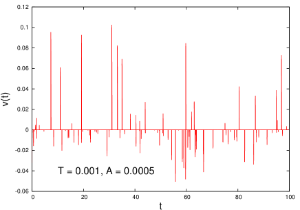
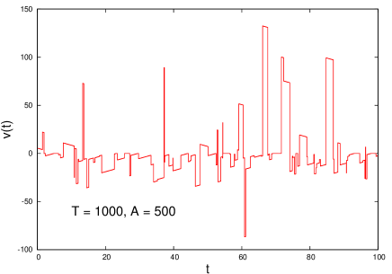
Figure 1: Left: Velocity vs time for the ratchet, when asymmetry is present and $\tau_{c}/\tau_{\Delta}\simeq 10^{3}$ (rare collisions limit). Simulations of the dynamics are performed using a $f(v)$ exponential, with different decay rates for positive or negative $v$. Right: same plot, with $\tau_{c}/\tau_{\Delta}\simeq 10^{-3}$ (frequent collisions limit). See caption of Fig. 2 for the definitions of $A$ and $T$.

Supposing the system to be ergodic, we can compute the stationary averages of the dynamical variables of the ratchet by performing their time average over long trajectories. The calculation of time averages is possible noticing that between two collisions the ratchet velocity is $v(t)=v_{0}-\sigma(v_{0})\Delta t$, where $v_{0}$ is the velocity after that collision; this motion introduces another time scale, the mean stopping time of the ratchet $\tau_{\Delta}=\langle|v|\rangle_{f}/\Delta$ (where we denote with $\langle\cdot\rangle_{f}$ the averages over the pdf $f(v)$). When $\tau_{c}\gg\tau_{\Delta}$, the ratchet generally stops before a new collision (rare collisions limit); viceversa, when $\tau_{c}\ll\tau_{\Delta}$ the ratchet is almost always in motion (frequent collisions limit). Simulated trajectories for both cases are shown in Fig. (1). Performing the time average, we find the average velocity of the ratchet

$$\langle v\rangle=\langle v\rangle_{f}-\bar{v}\langle\sigma(v)(1-e^{-|v|/\bar{v}})\rangle_{f},$$ (8)

where $\bar{v}=\Delta\tau_{c}$ is a characteristic velocity. Through the characteristic function $q(k)=\langle e^{ikv}\rangle$, it is possible to compute the stationary probability density of the velocity that is

$$P(v)=\int^{+\infty}_{-\infty}dv^{\prime}f(v^{\prime})\left\{e^{-|v^{\prime}|/\bar{v}}\delta(v)+\frac{\sigma(v^{\prime})}{\bar{v}}e^{(v-v^{\prime})\sigma(v^{\prime})/\bar{v}}\left[\Theta(v^{\prime}-v)-\Theta(-v)\right]\right\}$$ (9)

From Eq. (8), we notice that the second term in the rhs yields a net drift also if $\langle v\rangle_{f}=0$: this is the ratchet effect we are looking for. To observe it, it is necessary that $\Delta\neq 0$ (breaking of time reversal symmetry) and $f(v)\neq f(-v)$ (breaking of spatial symmetry). In the rare and the frequent collisions limits, if $\langle v\rangle_{f}=0$ we find respectively that

$$\tau_{c}\gg\tau_{\Delta}\quad \Rightarrow\quad\langle v\rangle\approx\frac{1}{2\bar{v}}\langle\sigma(v)\,v^{2}\rangle_{f}$$ (10a)

$$\tau_{c}\ll\tau_{\Delta}\quad \Rightarrow\quad\langle v\rangle\approx-\,\bar{v}\,\langle\sigma(v)\rangle_{f}$$ (10b)

so, depending on $f(v)$, the sign of the velocity can change by changing the parameters of the system. Furthermore, from Eq. (9), we point out the presence of a delta function into $P(v)$: its weight represents the finite time that the ratchet spends in $v=0$. Generally, the stationary pdf of the velocity for ratchet with Coulomb friction can be written as (Talbot et al. (2011))

$$P(v)=\gamma_{0}\delta(v)+\gamma_{R}P_{R}(v),$$ (11)

where $P_{R}(v)$ is a regular function of $v$. In our model, we obtain $\gamma_{0}=\left\langle e^{-v/\bar{v}}\right\rangle_{f}$, that goes to 1 in the rare collisions limit, and to 0 in the frequent collisions limit.

We simulate numerically the dynamics of the system, using a $f(v)$ exponential with different decay rates for $v$ positive or negative, finding perfect agreement between simulations and theory; some results are shown in Fig. (2), putting in evidence the asymptotic decays for $\langle v\rangle$ and $\gamma_{0}$ at large $T$.

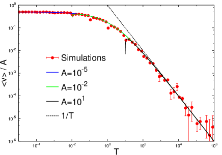
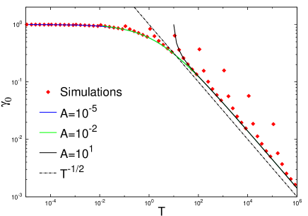
Figure 2: Left: Numerical simulations and analytical results for the average velocity of the ratchet, Eq.(8), rescaled by $A=\langle\sigma(v)v^{2}\rangle_{f}$, which characterizes the asymmetry of the system ($A=0$ for even $f(v)$). The temperatures $T$ are given by $T=\langle v^{2}\rangle_{f}$ (we are also assuming $\langle v\rangle_{f}=0$, and we set $\tau_{c}=\Delta=\bar{v}=1$, then $\tau_{\Delta}\simeq\sqrt{T}$. $f(v)$ is chosen as in Fig. (1). The dashed line represents the $T^{-1}$ asymptotic behavior predicted in this case for large values of $T$. Right: Numerical simulations and analytical results for $\gamma_{0}$. Same parameters as in left plot. The dotted line represents the $T^{-1/2}$ decay predicted in this case for large $T$.

III.3 The asymmetric Rayleigh piston

We study here the dynamics of an asymmetric Rayleigh piston, introduced in Alkemade et al. (1963), under the action of Coulomb friction Sarracino et al. (2013); Sano and Hayakawa (2014). In this model a piston of mass $1$, constrained to move along a given direction, interacts via elastic collisions with two gases of particles, which are placed on both sides of the piston (see Fig. 3). The particles of the two gases have different masses but are kept at the same temperature $T$. Therefore, in the absence of nonlinear friction, the whole system is at equilibrium at temperature $T$ and the spatial asymmetry introduced by the different masses cannot produce any rectification of fluctuations. On the contrary, when the motion of the piston is also subjected to Coulomb friction, dissipative effects intervene and a motor effect is observed.

The dynamics of the piston is described by Eq.(1), neglecting the spatial dependence ($U(x)\equiv 0$), with $J_{Lang}[v|P(v,t)]=0$ and $F_{nl}=-\Delta\sigma(v)$. Denoting by $m_{l}=\epsilon^{2}$ and $m_{r}=\alpha\epsilon^{2}$ the masses of particles at left and at right of the piston respectively, and by $p_{r}(u)$ and $p_{l}(u)$ their velocity distributions, where $u$ is the velocity of gas particles, the asymmetric transition rates appearing in the collision term $J_{col}[v|P(v,t)]$ are Alkemade et al. (1963)

$$W_{\epsilon}(v^{\prime}|v) = \left(\frac{1+\epsilon^{2}}{2\epsilon^{2}}\right)^{2}(v^{\prime}-v)$$

$$\times p_{l}\left(\frac{1+\epsilon^{2}}{2\epsilon^{2}}v^{\prime}-\frac{1-\epsilon^{2}}{2\epsilon^{2}}v\right),$$

$$W_{\epsilon}(v^{\prime}|v) = \left(\frac{1+\alpha\epsilon^{2}}{2\alpha\epsilon^{2}}\right)^{2}(v-v^{\prime})$$ (12)

$$\times p_{r}\left(\frac{1+\alpha\epsilon^{2}}{2\alpha\epsilon^{2}}v^{\prime}-\frac{1-\alpha\epsilon^{2}}{2\alpha\epsilon^{2}}v\right).$$

Notice that these transition rates satisfy DB with respect to the Gaussian distribution $P_{0}(v)=(2\pi T)^{-1/2}\exp(-v^{2}/2T)$ even when $\alpha\neq 1$ Alkemade et al. (1963).

In this model it is important to point out two time scales: $\tau_{\Delta}=v^{*}/\Delta=\sqrt{T}/\Delta$, which is the stopping time due to friction, and $\tau_{th}\simeq\sqrt{\pi/(2T)}/[2\rho(\sqrt{\epsilon^{2}}+\sqrt{\alpha\epsilon^{2}})]$, which is the thermalization time of the piston with the gas in the absence of friction (proportional to the mean collision time), where $\rho$ is the gas density (equal on both sides of the piston).

An analytical expression for the average drift can be obtained in the limit of rare collisions, namely when $\tau_{th}\gg\tau_{\Delta}$. In this case, assuming that every collision occurs when the piston is at rest, the average velocity can be computed using the Independent Kick Model (IKM) introduced in Talbot and Viot (2012); Talbot et al. (2011). For our model this yields

$$\langle v\rangle=\left(\int du|u|p_{r}(u)+\int du|u|p_{l}(u)\right)\int_{0}^{\tau}v(t)dt,$$ (13)

where $v(t)=v_{0}-\Delta\sigma(v_{0})t$, $\tau=|v_{0}|/\Delta$ and $v_{0}$ is the velocity after a collision: $v_{0}=v^{+}$ if $u>0$, and $v_{0}=v^{-}$ if $u<0$, where $v^{+}=\frac{2u}{1+1/(\alpha\epsilon^{2})}$ and $v^{-}=\frac{2u}{1+1/\epsilon^{2}}$. Using these expressions, and considering a gaussian distribution for $p_{r/l}(u)$ with variance $T/m_{r/l}$, one obtains

$$\langle v\rangle=\frac{2\rho}{\Delta}\sqrt{\frac{2T^{3}}{\pi}}\left[\frac{\sqrt{\epsilon^{2}}}{(\epsilon^{2}+1)^{2}}-\frac{\sqrt{\alpha\epsilon^{2}}}{(\alpha\epsilon^{2}+1)^{2}}\right].$$ (14)

Notice that the average velocity is finite when the asymmetry in the system is present (i.e. $\alpha\neq 1$). Notice also that in the limit $\epsilon\to 0$ the drift vanishes. In Fig. 3, right panel, the analytical prediction (14) of the IKM (black lines) is shown to be in perfect agreement with the numerical results (see Sarracino et al. (2013) for details) in the rare collision regime. Fig. 3, right panel, also shows $\langle v\rangle$ (black dots for $\epsilon^{2}=0.01$ and blue squares for $\epsilon^{2}=0.5$, with $\alpha=2$) for a large range of values of the ratio $\tau_{\Delta}/\tau_{th}$, which is varied by changing $\Delta$, with the other parameters fixed (see caption). A net drift is observed, as expected. It is interesting to notice that thermodynamic (bulk) pressures are equal in the two reservoirs and therefore the motion of the piston is due to the fact that the average exchanged momentum between gas and piston is not equal to bulk pressure. A recent theory about non-equilibrium momentum deficit Fruleux et al. (2012) is difficult to be applied in this particular case, as noticed recently by other authors Sano and Hayakawa (2014). Another interesting feature which appears in simulations, but is hardly explained by theory, is the presence of extremal points (even more than one) and current inversion points. A similar behavior is encountered in other models discussed here.

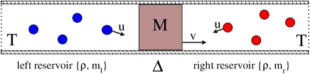
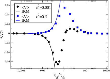
Figure 3: Left: a sketch of the asymmetric Rayleigh piston model (in this paper the piston mass $M$ is set to $1$). Right: Numerical simulations of the Rayleigh piston, with $T=10$, $\rho=0.5$, $\alpha=2$, showing $\langle v\rangle$ as a function of $\tau_{\Delta}/\tau_{th}$, for $\epsilon^{2}=0.01$ (black dots) and $\epsilon^{2}=0.5$ (blue squares). The continuous curves show the analytical predictions of the IKM, Eq. (14).

III.4 Rotator with an asymmetric shape

In this subsection, the tracer driven by the Brownian motor effect is a rotator, and for this reason we replace $x,v$ by $\theta,\omega$, i.e. angular displacement and angular velocity respectively. The rotator has momentum of inertia $I$, mass $1$ and radius of inertia $R_{I}=\sqrt{I}$. It is constituted by the set of material points with cartesian coordinates $\{x,y,z\}$ with $z\in[0,h]$ (where $h$ is its height) and $\sqrt{x^{2}+y^{2}}<r(s)$ for each $s\in[0,S]$ where $s$ is the curvilinear abscissa, $r(s)$ is the curve delimiting a section of the solid in the $\hat{xy}$ plane, and $S$ is the perimeter of the section. The rotator changes its angular velocity for two reason: 1) because of dry friction $F_{nl}=-\Delta\sigma(\omega)$, with $\Delta$ the frictional torque rescaled by momentum of inertia, and 2) for the effect of elastic collisions with a dilute gas of particles at equilibrium at temperature $T=\epsilon^{2}v_{0}^{2}$. The gas surrounding the rotator has volume number density $n$ and $\rho=nh$ is its two-dimensional projection, which is the only one which matters in the problem. Note that $\rho S\equiv n\Sigma$ with $\Sigma$ the total surface of the rotator parallel to the rotation axis. We finally assume that no external potential and no heat bath are present, i.e. Eq. (1) (with the replacements $x\to\theta$, $v\to\omega$) holds with $U\equiv 0$ and $\gamma=0$. A sketch of the model with used symbols is shown in Fig. 4, left panel.

The effect of the elastic collisions with the equilibrium gas is to change $\omega$ into $\omega^{\prime}$ and that of the colliding particle from ${\mathbf{u}}$ to ${\mathbf{u}}^{\prime}$, following the rule

$$\omega^{\prime} =\omega+2\frac{({\mathbf{v}}-{\mathbf{u}})\cdot\hat{n}}{R_{I}}\frac{g\epsilon^{2}}{1+\epsilon^{2}g^{2}},$$ (15a)

$${\mathbf{u}}^{\prime} ={\mathbf{u}}+2\frac{({\mathbf{v}}-{\mathbf{u}})\cdot\hat{n}}{1+\epsilon^{2}g^{2}}\hat{n}$$ (15b)

where ${\mathbf{v}}=\omega\hat{z}\times{\mathbf{r}}$ is the linear velocity of the rotator at the point of impact ${\mathbf{r}}$, $\hat{n}$ is the unit vector perpendicular to the surface at that point, and finally $g=\frac{{\mathbf{r}}\cdot\hat{t}}{R_{I}}$ with $\hat{t}=\hat{z}\times\hat{n}$ which is the unit vector tangent to the surface at the point of impact. Equations (15) guarantee that total angular momentum and total kinetic energy are conserved and that relative velocity projected on the collision unit vector is reflected. A few relations in cartesian coordinates may be useful: ${\mathbf{v}}=(-\omega r_{y},\omega r_{x})$ and $\hat{t}=(-n_{y},n_{x})$. It is also useful to realize that ${\mathbf{v}}\cdot\hat{n}=-\omega R_{I}g$, and to introduce the “equilibrium” angular velocity $\omega_{0}=\frac{\epsilon v_{0}}{R_{I}}$ and the rescaled velocity $\Omega=\frac{\omega}{\omega_{0}}$.

With the above collision rule, the transition rates $W_{\epsilon}$ take the explicit form

$$W(\omega^{\prime}|\omega)=\frac{\rho SR_{I}^{2}}{8\sqrt{2\pi}\epsilon^{2}v_{0}}\int\frac{ds}{S}|\omega^{\prime}-\omega|\frac{(1+\epsilon^{2}g^{2})^{2}}{\epsilon^{2}g^{2}}\\ \times\Theta\left[\frac{\omega^{\prime}-\omega}{g}\right]\exp\left[-\frac{R_{I}^{2}}{2\epsilon^{2}v_{0}^{2}}\left(\omega\epsilon g+\frac{(\omega^{\prime}-\omega)(1+\epsilon^{2}g^{2})}{2\epsilon g}\right)^{2}\right].$$ (16)

.

Following the same lines of the two previous sections, it is useful to realize that two time-scales are relevant in the system: 1) the mean stopping time due to environmental dissipation, which is dominated by dry friction (being almost always $\gamma_{a}|\omega|<\Delta$), $\tau_{\Delta}=\frac{\langle|\omega|\rangle_{pc}}{\Delta}\sim\frac{\epsilon v_{0}}{R_{I}\Delta}$, where $\langle\cdot\rangle_{pc}$ denotes a post-collisional average; 2) the mean free time between two collisions $\tau_{c}\sim\frac{1}{n\Sigma v_{0}}$. This implies the existence of a main control parameter

$$\beta^{-1}=\frac{\epsilon n\Sigma v_{0}^{2}}{\sqrt{2}\pi R_{I}\Delta}\approx\frac{\tau_{\Delta}}{\tau_{c}}$$ (17)

which is an estimate of the ratio of those two time-scales, as verified in simulations.

When the mass of the rotator is large, $\epsilon\ll 1$, and $\beta^{-1}\gg 1$, friction becomes negligible and the collisional noise becomes white noise, so that the average drift tends to zero. A finite drift could be achieved in the case of inelastic collisions, which has been considered elsewhere Gnoli et al. (2013a, c).

In the opposite limit $\beta^{-1}\ll 1$, an independent kicks approximation leads to the formula for the rescaled average velocity of the ratchet

$$\langle\Omega\rangle =\sqrt{\pi}4\beta^{-1}\epsilon^{2}\mathcal{A}_{RCL}$$ (18a)

$$\mathcal{A}_{RCL} =\left\langle\frac{\sigma(g)g^{2}}{(1+\epsilon^{2}g^{2})^{2}}\right\rangle_{surf},$$ (18b)

where $\mathcal{A}_{RCL}=0$ for symmetric shapes of the rotator. Above we have used the shorthand notation for the uniform average along the perimeter (denoted as “surface”) of a horizontal section of the rotator $\langle\rangle_{surf}=\int_{surf}\frac{ds}{S}$. Note that the limit $\Delta\to 0$ is singular in formula (18a), since in the absence of dissipation between collisions the stopping time becomes infinite, $\tau_{\Delta}\to\infty$, and the assumption of “rare collisions”, $\beta^{-1}\ll 1$, breaks down. The magnitude of the drift is predicted to increase with $\beta^{-1}$: this corresponds to $|\langle\omega\rangle|\sim v_{0}^{3}$.

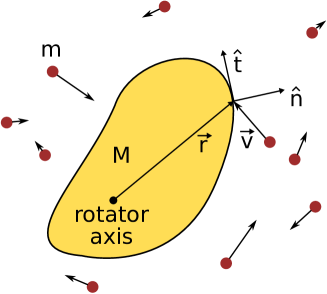
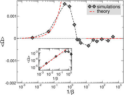
Figure 4: Left: sketch of the model. Right: results of numerical simulations for the rotator model with asymmetric shape, for different values of $\beta^{-1}$.

In Figure 4, right panel, we have shown the results of numerical simulations for the rotator model with a shape identical to the one used in recent granular experiments, see Ref. Gnoli et al. (2013a) for details. Both predictions for large and small values of $\beta^{-1}$ are well reproduced. As expected by interpolating the two predictions, the average drift velocity $\langle\Omega\rangle$ goes through a maximum. A still unexplained feature, common also to the Rayleigh piston case discussed previously, is the presence of a current inversion and a second extremal point (a minimum), before going asymptotically to zero at large $\beta^{-1}$.

IV Kramers equation with nonlinear friction

In this section we consider the effect of an asymmetric spatial potential $U(x)$, coupled to nonequilibrium conditions induced by the presence of nonlinear velocity-dependent forces $F_{nl}$ Sarracino (2013). In particular, we consider a ”generalized” Klein-Kramers equation for the motion of a particle of mass $m=1$, with position $x$ and velocity $v$, subjected to thermal fluctuations,

$$\dot{x}(t) = v(t)$$

$$\dot{v}(t) = -\gamma v(t)+F_{nl}[v(t)]-U^{\prime}[x(t)]+\eta(t),$$ (19)

where $\eta(t)$ is a white noise, with $\langle\eta(t)\rangle=0$ and $\langle\eta(t)\eta(t^{\prime})\rangle=2\gamma T\delta(t-t^{\prime})$, $\gamma$ and $T$ being two parameters and $\delta(t)$ the Dirac’s delta. The corresponding Fokker-Planck equation for this model is given by Eq. (1), with $J_{col}=0$.

We consider here the nonlinear force in the form of Coulomb friction, namely

$$F_{nl}[v(t)]=-\Delta\sigma[v(t)].$$ (20)

Without external potential, model (IV) with friction (20) has been studied for instance in de Gennes (2005); Hayakawa (2005); Daniel et al. (2005b); Plyukhin and Froese (2007); Baule et al. (2011).

We also consider a model for active Brownian particles Schweitzer et al. (1998), inspired by the Rayleigh-Helmholtz model for sustained sound waves Rayleigh (1945), where

$$F_{nl}[v(t)]=\gamma_{1}v(t)-\gamma_{2}v^{3}(t),$$ (21)

with $\gamma_{1}$ and $\gamma_{2}$ positive constants, and $\gamma=0$ in Eq. (IV). The motion of the particle is accelerated for small $v$ and is damped for high $v$. This model represents the internal energy conversion of the active particles.

The asymmetric ratchet potential is the one usually studied in the literature of Brownian motors Bartussek et al. (1994)

$$U(x)=\sin(x)+\mu\sin(2x),$$ (22)

where $\mu$ is an asymmetry parameter. In the case of frictional force (21) the effect of an asymmetric potential has been investigated in Schweitzer et al. (2000); Fiasconaro et al. (2008).

We have performed numerical simulations of the model (IV), which are reported in Fig. 5, left panel. Here we show the position of the Brownian particle in time, in the absence (continuous black line) and in the presence of Coulomb friction (dashed red line). Notice the strong rectification phenomenon occurring in the nonequilibrium case, namely when Coulomb friction is present.

In Fig. 5, right panel, we report the behavior of the system at varying the parameter $\mu$ of the asymettric potential. In the top panel we show the average velocity of the particle described by Eq. (IV) with Coulomb friction (20) and in the lower panel, we show the results of numerical simulations of the model for active particles described by Eq. (21). As expected, for $\mu=0$, the ratchet effect vanishes in both models, because the potential is spatially symmetric in that case. By increasing the value of $\mu$ a non-monotonic behavior is observed. The decreasing of the ratchet effect for large values of $\mu$ is probably due to the fact that the potential develops more than one minimum. This causes an overall slowing down of the dynamics and, therefore, of the average velocity.

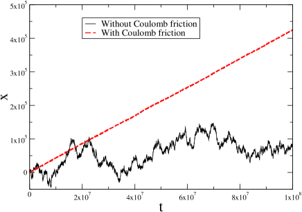
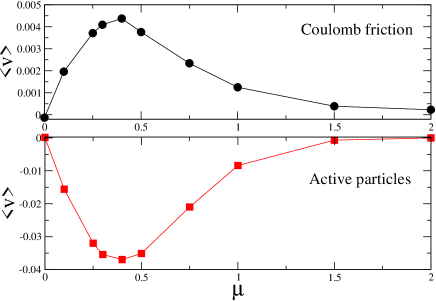
Figure 5: Left: Evolution in time of the position $x(t)$ for the model in Eq. (IV) without Coulomb friction (black continuous lines), with parameters $\gamma=0.05$, $\gamma T=0.5$, and $\mu=0.4$, and with Coulomb friction (red dashed line), with same parameters and $\Delta=1$. Right: Average drift for the model with Coulomb friction (20) (top panel) with parameters $\Delta=1$, $\gamma=0.05$, $\gamma T=0.5$, and for the model for active particles (21) (bottom panel) with parameters $\gamma_{1}=\gamma_{2}=1$, and $\gamma T=0.5$, as a function of the parameter $\mu$.

V Conclusions

We have reviewed a few models of Markovian Brownian motors: the common ingredient is non-linear friction as the only mechanism for energy dissipation. All other features, such as an external potential as well as thermostats at the same temperature, are of “equilibrium” nature. Our focus is on a particular choice of non-linear friction, which is found in many macroscopic experiments, that is Coulomb friction between dry surfaces. The interplay between non-linear friction and the other (deterministic and stochastic) forces acting on the motor is subtle and not always generates a motor effect. We have shown two possible routes toward rectification: they go through the presence of thermal non-white noise (e.g. collisions with a gas at equilibrium) or through the introduction of spatial inhomogeneity (e.g. an external potential). What is common between these two mechanisms is that they grant to the system a larger set of possible trajectories (with respect to white noise in homogeneous space). In this larger set, cyclic trajectories are accessible which guarantee probability currents and (in the presence of a spatial asymmetry) a motor effect. Apart from the simplest model discussed in section III.B, full analytical treatment of these models is missing, and expressions for the drift are known only in particular limits. Far from these limits, numerical simulations suggest a rich and complex behavior, with extremal and inversion points in the drift as a function of the models’ parameters, which are still lacking a satisfying explanation.