Exponentiated Weibull-logarithmic Distribution: Model, Properties and Applications

Abstract

In this paper, we introduce a new four-parameter generalization of the exponentiated Weibull (EW) distribution, called the exponentiated Weibull-logarithmic (EWL) distribution, which obtained by compounding EW and logarithmic distributions. The new distribution arises on a latent complementary risks scenario, in which the lifetime associated with a particular risk is not observable; rather, we observe only the maximum lifetime value among all risks. The distribution exhibits decreasing, increasing, unimodal and bathtub-shaped hazard rate functions, depending on its parameters and contains several lifetime sub-models such as: generalized exponential-logarithmic (GEL), complementary Weibull-logarithmic (CWL), complementary exponential-logarithmic (CEL), exponentiated Rayleigh-logarithmic (ERL) and Rayleigh-logarithmic (RL) distributions. We study various properties of the new distribution and provide numerical examples to show the flexibility and potentiality of the model.

1 Introduction

In biological and engineering sciences study of length of organisms, devices and materials is of major important. A substantial part of such study is devoted to modeling the lifetime data by a failure distribution. The Weibull and EW distributions are the most commonly used distributions in reliability and life testing. These distributions have several desirable properties and nice physical interpretations. Unfortunately, however, these distributions do not provide a reasonable parametric fit for some practical applications where the underlying hazard functions may be decreasing, unimodal and bathtub-shaped.

Recently, there has been a great interest among statisticians and applied researchers in constructing flexible families of distributions to facilitate better modeling of data. The exponential-geometric (EG), exponential-Poisson (EP), exponential-logarithmic (EL), exponential-power series (EPS), Weibull-geometric (WG), Weibull-power series (WPS), exponentiated exponential-Poisson (EEP), complementary exponential-geometric (CEG), Poisson-exponential (PE), generalized exponential-power series (GEPS), exponentiated Weibull-geometric (EWG) and exponentiated Weibull-Poisson (EWP) distributions were introduced and studied by Adamidis and Loukas [2], Kus [24], Tahmasbi and Rezaei [38], Chahkandi and Ganjali [11], Barreto-Souza et al. [8] and Morais and Barreto-Souza [31], Barreto-Souza and Cribari-Neto [6], Louzada-Neto et al. [25], Cancho et al. [10], Mahmoudi and Jafari [26], Mahmoudi and Shiran [27] and Mahmoudi and Sepahdar [28], respectively.

In this paper, we propose a new four-parameters distribution, referred to as the EWL distribution, which contains as special sub-models the generalized exponential-logarithmic (GEL), complementary Weibull-logarithmic (CWL), complementary exponential-logarithmic (CEL), exponentiated Rayleigh-logarithmic (ERL) and Rayleigh-logarithmic (RL) distributions, among others. The paper is organized as follows: In Section 2, a new lifetime distribution, called the exponentiated Weibull-logarithmic (EWL) distribution, is obtained by mixing exponentiated Weibull and logarithmic distributions. Various properties of the proposed distribution are discussed in Section 3. Estimation of the parameters by maximum likelihood via a EM-algorithm and inference for large sample are presented in Section 4. In Section 5, we studied some special sub-models of the EWL distribution. Finally, in Section 6, experimental results of the proposed distribution, based on two real data sets, are illustrated.

2 The proposed distribution

Suppose that the random variable $X$ has the EW distribution where its cdf and pdf are given by

$$F_{X}(x)=\left(1-e^{-(\beta x)^{\gamma}}\right)^{\alpha},$$ (1)

and

$$f_{X}(x)=\alpha\gamma\beta^{\gamma}x^{\gamma-1}e^{-(\beta x)^{\gamma}}\left(1-e^{-(\beta x)^{\gamma}}\right)^{\alpha-1},$$ (2)

respectively, where $x>0$, $\alpha>0$, $\beta>0$ and $\gamma>0$. Given $N$, let $X_{1},\cdots,X_{N}$ be independent and identify distributed random variables from EW distribution. Let $N$ is distributed according to the logarithmic distribution with pdf

$$P(N=n)=\frac{\theta^{n}‎}{-n\log(1-‎\theta‎)},~{}n=1,2,\cdots,~{}\theta>0.$$

Let $Y=\max(X_{1},\cdots,X_{N})$, then the conditional cdf of $Y|N=n$ is given by

$$F_{Y|N=n}(y)=[1-e^{-(‎\beta y‎)^{‎\gamma‎}}]^{n‎\alpha‎},$$ (3)

which is a EW distribution with parameters $n\alpha$, $\beta$, $\gamma$. The EWL distribution that is defined by the marginal cdf of $Y$, is given by

$$F(y)=‎‎‎\frac{\log\big{[}1-‎\theta‎‎‎‎‎\big{(}1-e^{-(‎\beta y‎)^{‎\gamma‎}}\big{)}^{‎\alpha‎}\big{]}}{\log\big{(}1-‎\theta‎\big{)}}.$$ (4)

The pdf of EWL, denoted by EWL$(\alpha,\beta,\gamma,\theta)$, is given by

$$f(y)=\frac{\alpha\theta\gamma\beta^{\gamma}y^{‎\gamma-1‎}e^{-‎(\beta y‎)^{‎\gamma‎}}\big{(}1-e^{-‎(\beta y‎)^{‎\gamma‎}}\big{)}^{‎\alpha-1‎}‎}{\log(1-‎\theta‎)\big{(}‎\theta‎(1-e^{-‎(\beta y‎)^{‎\gamma‎}})^{‎\alpha‎}-1\big{)}}.$$ (5)

The graphs of EWL probability density function are displayed in Fig. 1 for selected parameter values.

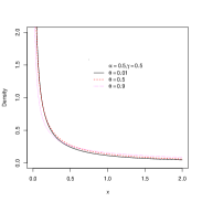
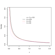
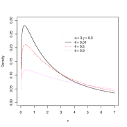
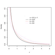
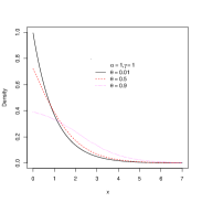
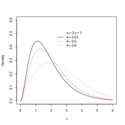
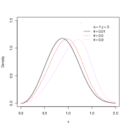
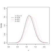
Figure 1: Plots of probability density function of EWL distribution for $\beta=1$ and different values $\alpha$, $\gamma$, and $\theta$.

3 Properties of the distribution

The probability density function of EWL distribution, which is given in (5), tending to zero as $y\rightarrow\infty$. The EWL leads to EW distribution as $\theta\rightarrow 0$. The following values of the parameters $\alpha$, $\beta$, $\gamma$ and $\theta$ are of particular interest: (i) $\gamma=1$, EWL reduces to GEL, which introduced and examined by Mahmoudi and Jafari [26]; (ii) $\alpha=1$, EWL reduces to CWL; (iii) $\alpha=\gamma=1$, EWL reduces to CEL, our approach here is complementary to that of Tahmasbi and Rezaei [38] in the sense that they consider the distribution $\min(X_{1},X_{2}...,X_{N})$ while we deal with $\max(X_{1},X_{2}...,X_{N})$; (iv) $\alpha=1$ and $\theta\rightarrow 0$, EWL reduces to Weibull; (v) $\gamma=1$ and $\theta\rightarrow 0$, EWL reduces to GE.

3.1 Quantiles and moments of the EWP distribution

The $\xi$th quantile of the EWL distribution, which is used for data generation from the EWL, is given by

$$x_{\xi}=\frac{1}{\beta}\big{[}-\log(1-(\frac{1-(1-\theta)^{\xi}}{\theta})^{1/\alpha})\big{]}^{1/\gamma}.$$ (6)

Now we obtain the moment generating function (mgf) and $k$th order moment of EWL distribution, since some of the most important features and characteristics such as tending, dispersion, skewness and kurtosis can be studied through these quantities. For a random variable $Y$ with EWL distribution the mgf is given by

$$\begin{array}[b]{ll}M_{Y}(t)=\frac{‎\alpha\theta}{\log(1-\theta)}\sum^{\infty}_{n=1}\sum^{\infty}_{k=0}\sum^{\infty}_{j=0}(-1)^{j+1}\frac{t^{k}\theta^{n-1}}{\beta^{k}k!}\Gamma(1+\frac{k}{\gamma}){n\alpha-1\choose j}(j+1)^{-(1+\frac{k}{\gamma})}.\end{array}$$ (7)

$M_{Y}(t)$ in (7) can be used to obtain the $k$th order moment of EWL distribution. We have

$$\begin{array}[b]{ll}E(Y^{k})=\frac{\alpha\theta\Gamma(1+\frac{k}{\gamma})}{\beta^{k}\log(1-‎\theta‎)}\sum^{\infty}_{n=1}\sum^{\infty}_{j=0}(-1)^{j+1}{n\alpha-1\choose j}\theta^{n-1}(j+1)^{-(1+\frac{k}{\gamma})}.\end{array}$$ (8)

Proposition 1

The random variable $Y$ with pdf given by (5) has mean and variance given, respectively, by

$$E(Y)=\frac{\alpha\theta\Gamma(1+\frac{1}{\gamma})}{\beta\log(1-‎\theta‎)}\sum^{\infty}_{n=1}\sum^{\infty}_{j=0}(-1)^{j+1}\theta^{n-1}{n\alpha-1\choose j}(j+1)^{-(1+\frac{1}{\gamma})},$$ (9)

and

$$\begin{array}[b]{ll}Var(Y)=\frac{\alpha\theta\Gamma(1+\frac{2}{\gamma})}{\beta^{2}\log(1-‎\theta‎)}\sum^{\infty}_{n=1}\sum^{\infty}_{j=0}(-1)^{j+1}\theta^{n-1}{n\alpha-1\choose j}(j+1)^{-(1+\frac{2}{\gamma})}-E^{2}(Y),\end{array}$$ (10)

where $E(Y)$ is given in Eq. (9).

3.2 The survival, hazard and mean residual life functions

Using (4) and (5), survival function (also known as reliability function) and hazard function (also known as failure rate function) of the EWL distribution are given, respectively, by

$$S(y)=1-F(y)=1-‎\frac{\log\big{(}1-‎\theta‎(1-e^{-‎(\beta y‎)^{‎\gamma‎}})^{‎\alpha‎}\big{)}}{\log(1-‎\theta‎)}‎,~{}~{}y>0,$$ (11)

and

$$h(y)=‎‎\frac{‎\alpha‎\theta‎‎\gamma‎\beta^{‎\gamma‎}y^{‎\gamma-1‎}e^{-‎(\beta y‎)^{‎\gamma‎}}\big{(}1-e^{-‎(\beta y‎)^{‎\gamma‎}}\big{)}^{‎\alpha-1‎}‎‎‎}{\big{(}‎\theta‎(1-e^{-‎(\beta y‎)^{‎\gamma‎}})^{‎\alpha‎}-1\big{)}\big{[}\log(1-‎\theta‎)-\log\big{(}1-‎\theta‎(1-e^{-‎(\beta y‎)^{‎\gamma‎}})^{‎\alpha‎}\big{)}\big{]}}‎$$ (12)

Proposition 2

The limiting behavior of hazard function of EWL distribution in (12) is
(i) for $0<\gamma<1$, $\lim_{y\rightarrow 0}h(y)=\left\{\begin{array}[]{lc}\infty&0<\alpha\leq 1\\ 0&\alpha>1,\end{array}\right.$ and $\lim_{y\rightarrow\infty}h(y)=0.$
(ii) for $\gamma=1$, $\lim_{y\rightarrow 0}h(y)=\left\{\begin{array}[]{lc}\infty&0<\alpha<1\\ -\frac{\theta\beta}{\log(1-\theta)}&\alpha=1\\ 0&\alpha>1,\end{array}\right.$ and $\lim_{y\rightarrow\infty}h(y)=\beta.$
(iii) for $\gamma>1$, $\lim_{y\rightarrow 0}h(y)=0,$ for each value $\alpha>0$ and $\lim_{y\rightarrow\infty}h(y)=\infty$.

Proof 1

The proof is a forward calculation and is omitted.

The graphs of hazard rate function of EWL distribution for $\beta=1$ and various values $\alpha$, $\gamma$ and $\theta$ are displayed in Fig. 2.

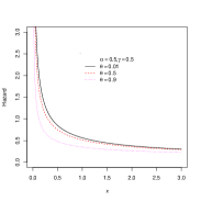
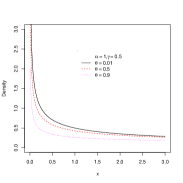
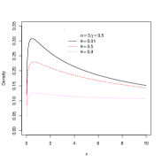
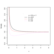
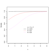
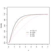
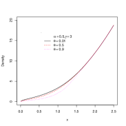
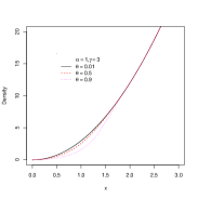
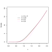
Figure 2: Plots of hazard rate function of EWL distribution for $\beta=1$ and different values $\alpha$, $\gamma$, and $\theta$.

Given that a component survives up to time $t\geq 0$, the residual life is the period beyond $t$ until the time of failure and defined by the conditional random variable $X-t|X>t$. The mean residual life (MRL) function is an important function in survival analysis, actuarial science, economics and other social sciences and reliability for characterizing lifetime. In reliability, it is well known that the MRL function and ratio of two consecutive moments of residual life determine the distribution uniquely (Gupta and Gupta, [19]).

In what seen this onwards we use the equations

$$\int_{t}^{\infty}y^{\gamma+s-1}e^{-(k+1)(\beta x)^{\gamma}}dy=\frac{1}{\gamma\beta^{‎\gamma+s‎}}(k+1)^{-(1+\frac{s}{\gamma})}\Phi(1+\frac{s}{\gamma};(k+1)(\beta t)^{\gamma}),$$

and

$$\int_{0}^{t}y^{\gamma+s-1}e^{-(k+1)(\beta x)^{\gamma}}dy=\frac{1}{\gamma\beta^{\gamma+s}}(k+1)^{-(1+\frac{i}{\gamma})}\gamma(1+\frac{s}{\gamma};(k+1)(\beta t)^{\gamma}),$$

where $\Phi(s;t)=\int_{t}^{\infty}x^{s-1}e^{-x}dx$ is the upper incomplete gamma function and $\gamma(s;t)=\int_{0}^{t}x^{s-1}e^{-x}dx$ is the lower incomplete gamma function. The $r$th order moment of the residual life of the EWL distribution, which is obtain via the general formula

$$m_{r}(t)=E\left[(Y-t)^{r}|Y>t\right]=\frac{1}{S(t)}\int_{t}^{\infty}(y-t)^{r}f(y)dy,$$

where $S(t)$ is the survival function, is given by

$$\begin{array}[b]{ll}m_{r}(t)&=‎\frac{‎\alpha‎\theta‎‎}{S(t)\log(1-‎\theta‎)}\sum_{i=0}^{r}\sum_{j=0}^{\infty}‎\sum_{k=0}^{\infty}‎(-1)^{r+k-i+1}t^{r-i}‎\theta^{j‎}\beta^{-i‎}(k+1)‎^{-(1+‎\frac{i}{‎\gamma‎}‎)}‎{{r}\choose{i}}{{\alpha(j+1)-1}\choose{k}}‎\vskip 6.0pt plus 2.0pt minus 2.0pt\\ &~{}~{}\times\Phi(1+\frac{i}{\gamma};(k+1)(\beta t)^{\gamma}),\end{array}$$ (13)

where $S(t)$ (the survival function of $Y$) is given in (11).
The MRL function of EWL obtain by setting $r=1$ in Eq. (13). MRL function as well as failure rate function is very important since each of them can be used to determine a unique corresponding life time distribution. Life times can exhibit IMRL (increasing MRL) or DMRL (decreasing MRL). MRL functions that first decreases (increases) and then increases (decreases) are usually called bathtub (upside-down bathtub) shaped, BMRL (UMRL).

Theorem 1

The MRL function of the EWL distribution is given by

$$\begin{array}[b]{ll}m_{1}(t)&=\frac{‎\alpha‎\theta}{S(t)\beta\log(1-‎\theta‎)}\sum_{j=0}^{\infty}\sum_{k=0}^{\infty}(-1)^{k+1}‎\theta^{j}{{\alpha(j+1)-1}\choose{k}}(k+1)^{-(1+\frac{1}{\gamma})}‎\vskip 6.0pt plus 2.0pt minus 2.0pt\\ &~{}~{}\times\Phi(1+‎\frac{1}{‎\gamma‎}‎;(k+1)(‎\beta t‎)^{‎\gamma‎})-t.\end{array}$$ (14)

The variance of the residual life of the EWL distribution can be obtained easily using $m_{2}(t)$ and $m_{1}(t)$.
On the other hand, the reversed residual life can be defined as the conditional random variable $t-X|X\leq t$ which denotes the time elapsed from the failure of a component given that its life is less than or equal to t. This random variable may also be called the inactivity time (or time since failure); for more details one can see Kundu and Nanda (2010) and Nanda et al., (2003). Using (5) and (11), the reversed failure (or reversed hazard) rate function of the EWL is given by

$$r(y)=\frac{f(y)}{F(y)}=‎‎\frac{‎\alpha‎\theta‎\gamma‎\beta^{‎\gamma‎}‎‎‎‎y^{‎\gamma-1‎}e^{-(‎\beta y‎)^{‎\gamma‎}}\big{(}1-e^{-(‎\beta y‎)^{‎\gamma‎}}\big{)}^{‎\alpha-1‎}}{\big{(}‎\theta(1-e^{-(‎\beta y‎)^{‎\gamma‎}})‎^{‎\alpha‎}-1\big{)}\log\big{[}1-‎\theta(1-e^{-(‎\beta y‎)^{‎\gamma‎}})‎^{‎\alpha‎})‎\big{]}}‎‎‎.$$

The $r$th order moment of the reversed residual life can be obtained by the well known formula

$$\mu_{r}(t)=E\left[(t-Y)^{r}|Y\leq t\right]=\frac{1}{F(t)}\int_{0}^{t}(t-y)^{r}f(y)dy,$$

hence,

$$\begin{array}[b]{ll}\mu_{r}(t)&=\frac{‎\alpha‎\theta‎‎}{F(t)\log(1-‎\theta‎)}\sum_{i=0}^{r}\sum_{j=0}^{\infty}\sum_{k=0}^{\infty}‎\frac{(-1)^{i+k+1}‎\theta^{j‎}t^{r-i}‎‎}{\beta^{i}(k+1)^{1+‎‎\frac{i}{‎\gamma‎}‎‎}}{{r}\choose{i}}{{(j+1)‎\alpha-1‎}\choose{k}}‎\gamma‎(1+‎\frac{i}{‎\gamma‎};(k+1)(‎\beta t‎)^{‎\gamma‎}).\end{array}$$ (15)

The mean and second moment of the reversed residual life of the EWL distribution can be obtained by setting $r=1,~{}2$ in (15). Also, using $\mu_{1}(t)$ and $\mu_{1}(t)$ we obtain the variance of the reversed residual life of the EWL distribution.

3.3 Mean deviations from the mean and median

The amount of scatter in a population can be measured by the totality of deviations from the mean and median. The mean deviation from the mean is a robust statistic, being more resilient to outliers in a data set than the standard deviation. The mean deviation from the median is a measure of statistical dispersion. It is a more robust estimator of scale than the sample variance or standard deviation.

For a random variable $X$ with pdf $f(x)$, cdf $F(x)$, mean $\mu=E(X)$ and $M=Median(X)$, the mean deviation about the mean and the mean deviation about the median are defined by

$$\delta_{1}(X)=\int_{0}^{\infty}|x-\mu|f(x)dx=2\mu F(\mu)-2I(\mu)$$

and

$$\delta_{2}(X)=\int_{0}^{\infty}|x-M|f(x)dx=2MF(M)-M+\mu-2I(M),$$

respectively, where $I(b)=\int^{b}_{0}xf(x)dx$

Theorem 2

The Mean deviations function of the EWL distribution are

$$\begin{array}[b]{ll}\delta_{1}(X)&=\frac{2}{\log(1-‎\theta)‎}\Big{[}\mu\log\left(1-‎\theta(1-e^{-(‎\beta‎\mu‎‎)^{‎\gamma‎}})‎^{‎\alpha‎}\right)+\alpha\theta\beta^{-1}\sum_{j=0}^{\infty}\sum_{k=0}^{\infty}(-1)^{k}\frac{\theta^{j}}{(k+1)^{1+\frac{1}{\gamma}}}{{\alpha(j+1)-1}\choose{k}}‎\\ &~{}~{}~{}\times‎\gamma(1+\frac{1}{\gamma};(k+1)(\beta\mu)^{\gamma})\Big{]},\end{array}$$

and

$$\delta_{2}(X)=\mu+\frac{2\alpha\theta}{\beta\log(1-‎\theta)‎)}\sum_{j=0}^{\infty}\sum_{k=0}^{\infty}(-1)^{k}\frac{\theta^{j}}{(k+1)^{1+\frac{1}{\gamma}}}{{\alpha(j+1)-1}\choose{k}}‎‎\gamma(1+\frac{1}{\gamma};(k+1)(\beta M)^{\gamma}),$$

where $\mu$ is given in (9) and $M$ is obtained by setting $\xi=.5$ in (6).

3.4 Bonferroni and Lorenz curves

The Bonferroni and Lorenz curves and Gini index have many applications not only in economics to study income and poverty, but also in other fields like reliability, medicine and insurance. The most remarkable property of the Bonferroni index is that it overweights income transfers among the poor, and the weights are higher the lower the transfers occur on the income distribution. Hence, it is a good measure of inequality when changes in the living standards of the poor are concerned. There are many problems especially in labor economics that fall into this category. Using a version of the assignment model, we show that the Bonferroni index can be formulated endogenously within a mechanism featuring efficient assignment of workers to firms. This formulation is useful in evaluating the interactions between the distribution of skills and earnings inequality with a special emphasis on the lower tail of the earnings distribution. Moreover, it allows us to think about earnings inequality by separately analyzing the contribution of each economic parameter.

The Bonferroni curve $B_{F}[F(x)]$ is given by

$$B_{F}[F(x)]=\frac{1}{\mu F(x)}\int^{x}_{0}uf(u)du,$$

or equivalently given by $B_{F}[p]=\frac{1}{\mu p}\int^{p}_{0}F^{-1}(t)dt$ where $p=F(x)$ and $F^{-1}(t)=\inf\{x:F(x)\geq t\}.$ The Bonferroni and Lorenz curves of the EWL distribution are given, respectively, by

$$\begin{array}[]{ll}B_{F}[F(x)]&=\frac{-\alpha\theta}{\beta\mu\log\left(1-‎\theta(1-e^{-(‎\beta x‎)^{‎\gamma‎}})‎^{‎\alpha‎}\right)}\sum_{j=0}^{\infty}\sum_{k=0}^{\infty}(-1)^{k}\frac{\theta^{j}}{(k+1)^{1+\frac{1}{\gamma}}}{{\alpha(j+1)-1}\choose{k}}‎\\ &~{}~{}~{}\times‎\gamma(1+\frac{1}{\gamma};(k+1)(\beta x)^{\gamma}),\end{array}$$

and

$$\begin{array}[]{ll}L_{F}[F(x)]&=B_{F}[F(x)]F(x)=\frac{-\alpha\theta}{\beta\mu\log\left(1-‎\theta‎\right)}\sum_{j=0}^{\infty}\sum_{k=0}^{\infty}(-1)^{k}\frac{\theta^{j}}{(k+1)^{1+\frac{1}{\gamma}}}{{\alpha(j+1)-1}\choose{k}}‎\\ &~{}~{}~{}\times‎\gamma(1+\frac{1}{\gamma};(k+1)(\beta x)^{\gamma}),\end{array}$$

where $\mu$ is the mean of EWL distribution.
The scaled total time on test transform of a distribution function $F$ is defined by

$$S_{F}[F(t)]=\frac{1}{\mu}\int^{t}_{0}S(u)du.$$

If $F(t)$ denotes the cdf of EWL distribution then

$$S_{F}[F(t)]=\frac{1}{\mu}\big{[}t-\frac{1}{\gamma\beta}\sum_{i=0}^{\infty}\sum_{k=0}^{\infty}\frac{(-1)^{i+1}\theta^{k}}{ki^{1/\gamma}}{{\alpha k}\choose{i}}\Phi(\frac{1}{\gamma};i(\beta t)^{\gamma})\big{]}.$$

The cumulative total time can be obtained by using formula $C_{F}=\int_{0}^{1}S_{F}[F(t)]f(t)dt$ and the Gini index can be derived from the relationship $G=1-C_{F}$.

3.5 Rényi and Shannon entropies of the EWL distribution

Entropy has been used in various situations in science and engineering. The entropy of a random variable $Y$ is a measure of variation of the uncertainty. Statistical entropy is a probabilistic measure of uncertainty or ignorance about the outcome of a random experiment, and is a measure of a reduction in that uncertainty. Numerous entropy and information indices, among them the Rényi entropy, have been developed and used in various disciplines and contexts. For a random variable with the pdf $f$, the Rényi entropy is defined by

$$I_{R}(r)=\frac{1}{1-r}\log\left[\int_{\mathbb{R}}f^{r}(y)dy\right],$$ (16)

for $r>0$ and $r\neq 1$. Using the power series expansion $(1-z)^{\alpha}=\sum_{0}^{\infty}(-1)^{j}{\alpha\choose j}z^{j}$ and change of variable $(\beta y)^{\gamma}=u$, we have

$$\int^{\infty}_{0}f^{r}(y)dy=\left[\frac{\alpha\theta}{\log(1-\theta)}\right]^{r}(\gamma\beta)^{r-1}\sum^{\infty}_{j=0}\sum^{\infty}_{k=0}(-1)^{k+r}{\alpha(r+j)-r\choose{k}}\frac{\theta^{j}\Gamma(r+j)}{j!\Gamma(r)}\frac{\Gamma\left(\frac{r(\gamma-1)+1}{\gamma}\right)}{(k+r)^{\frac{r(\gamma-1)+1}{\gamma}}}.$$ (17)

Thus, according to definition (16), the Rényi entropy of EWL distribution is given by

$$\begin{array}[b]{ll}I_{R}(r)&=\frac{1}{1-r}\log\Big{[}\left(\frac{\alpha\theta}{\log(1-\theta)}\right)^{r}(\gamma\beta)^{r-1}\sum^{\infty}_{j=0}\sum^{\infty}_{k=0}(-1)^{k+r}{\alpha(r+j)-r\choose{k}}\frac{\theta^{j}\Gamma(r+j)}{j!\Gamma(r)}\vskip 6.0pt plus 2.0pt minus 2.0pt\\ &~{}~{}\times\frac{\Gamma\left(\frac{r(\gamma-1)+1}{\gamma}\right)}{(k+r)^{\frac{r(\gamma-1)+1}{\gamma}}}\Big{]}.\end{array}$$ (18)

The Shannon entropy is defined by $E\left[-\log(f(Y))\right]$. This is a special case derived from $\lim_{r\rightarrow 1}I_{R}(r)$.

4 Estimation and inference

In this section, we discuss the estimation of the parameters of EWL distribution. Let $Y_{1},Y_{2},\cdots,Y_{n}$ be a random sample with observed values $y_{1},y_{2},\cdots,y_{n}$ from a EWL distribution with parameters $\alpha,\beta,\gamma$ and $\theta$. Let $\Theta=(\alpha,\beta,\gamma,\theta)^{T}$ be the parameter vector. The total log-likelihood function is given by

$$\begin{array}[b]{ll}l_{n}\equiv l_{n}(y;\Theta)&=n\log‎\alpha‎+n\log‎‎\theta‎+n\log‎‎\gamma‎+n‎\gamma‎\log‎‎\beta‎+‎(\gamma-1)‎\sum^{n}_{i=1}\log y_{i}\vskip 6.0pt plus 2.0pt minus 2.0pt\\ &~{}~{}~{}-\sum^{n}_{i=1}(‎\beta y_{i}‎)^{\gamma}+(‎\alpha-1‎)‎\sum^{n}_{i=1}\log(1-e^{-(‎\beta y_{i}‎)^{‎\gamma‎}})\vskip 6.0pt plus 2.0pt minus 2.0pt\\ &~{}~{}~{}-‎\sum^{n}_{i=1}\log\left(‎\theta‎(1-e^{-(‎\beta y_{i})^{‎\gamma‎}})^{‎\alpha‎}-1\right)-n\log\left(\log(1-‎\theta‎)\right).\end{array}$$

The associated score function is given by $U_{n}(\Theta)=(\partial l_{n}/\partial\alpha,\partial l_{n}/\partial\beta,\partial l_{n}/\partial\gamma,\partial l_{n}/\partial\theta)^{T}$, where

$$\begin{array}[]{ll}\frac{\partial l_{n}}{\partial\alpha}&=‎\frac{n}{‎\alpha‎}+\sum^{n}_{i=1}\log(1-e^{-(‎\beta y_{i}‎)^{‎\gamma‎}})-‎\theta‎‎\sum^{n}_{i=1}‎\frac{‎\log(1-e^{-(‎\beta y_{i}‎)^{‎\gamma‎}})(1-e^{-(‎\beta y_{i}‎)^{‎\gamma‎}})^{‎\alpha‎}‎}{‎\theta‎(1-e^{-(‎\beta y_{i}‎)^{‎\gamma‎}})^{‎\alpha‎}-1},\vskip 6.0pt plus 2.0pt minus 2.0pt‎\\ \frac{\partial l_{n}}{\partial\beta}&=‎\frac{n‎\gamma‎}{‎\beta‎}-‎\gamma‎\beta^{‎\gamma-1‎}\sum^{n}_{i=1}y_{i}^{‎\gamma‎}+(‎\alpha-1‎)‎‎\gamma‎\beta^{‎\gamma-1‎}‎‎\sum^{n}_{i=1}‎\frac{y_{i}^{‎\gamma‎}e^{-(‎\beta y_{i}‎)^{‎\gamma‎}}}{1-e^{-(‎\beta y_{i}‎)^{‎\gamma‎}}}\vskip 6.0pt plus 2.0pt minus 2.0pt\\ &~{}~{}-‎\theta‎\gamma‎\alpha‎‎\beta^{‎\gamma-1‎}‎‎‎‎‎‎‎‎‎\sum^{n}_{i=1}‎\frac{y_{i}^{‎\gamma‎}e^{-(‎\beta y_{i}‎)^{‎\gamma‎}}(1-e^{-(‎\beta y_{i}‎)^{‎\gamma‎}})^{‎\alpha-1‎}}{\theta‎(1-e^{-(‎\beta y_{i}‎)^{‎\gamma‎}})^{‎\alpha‎}-1}‎,\vskip 6.0pt plus 2.0pt minus 2.0pt\\ \frac{\partial l_{n}}{\partial\gamma}&=‎\frac{n}{‎\gamma‎}+n\log‎\beta+\sum^{n}_{i=1}\log y_{i}-\sum^{n}_{i=1}(‎\beta y_{i}‎)^{‎\gamma‎}\log(‎\beta y_{i}‎)\vskip 6.0pt plus 2.0pt minus 2.0pt\\ &~{}~{}‎‎+(‎\alpha-1‎)\sum^{n}_{i=1}‎\frac{(‎\beta y_{i}‎)^{‎\gamma‎}\log(‎\beta y_{i}‎)‎‎e^{-(‎\beta y_{i}‎)^{‎\gamma‎}}}{1-e^{-(‎\beta y_{i}‎)^{‎\gamma‎}}}-‎\theta‎\alpha\sum^{n}_{i=1}‎\frac{(‎\beta y_{i}‎)^{‎\gamma‎}\log(‎\beta y_{i}‎)e^{-(‎\beta y_{i}‎)^{‎\gamma‎}}(1-e^{-(‎\beta y_{i}‎)^{‎\gamma‎}})^{‎\alpha-1‎}}{\theta‎(1-e^{-(‎\beta y_{i}‎)^{‎\gamma‎}})^{‎\alpha‎}-1}‎,‎‎‎\vskip 6.0pt plus 2.0pt minus 2.0pt\\ \frac{\partial l_{n}}{\partial\theta}&=‎\frac{n}{‎\theta‎}-\sum^{n}_{i=1}‎\frac{(1-e^{-(‎\beta y_{i}‎)^{‎\gamma‎}})^{‎\alpha‎}}{\theta‎(1-e^{-(‎\beta y_{i}‎)^{‎\gamma‎}})^{‎\alpha‎}-1}‎+‎\frac{n}{(1-‎\theta‎)\log(1-‎\theta‎)}‎‎.\end{array}$$

The maximum likelihood estimation (MLE) of $\Theta$, say $\widehat{\Theta}$, is obtained by solving the nonlinear system $U_{n}\left(\Theta\right)=\textbf{0}$. The solution of this nonlinear system of equation has not a closed form. For interval estimation and hypothesis tests on the model parameters, we require the information matrix. The $4\times 4$ observed information matrix is

$$I_{n}\left(\Theta\right)=-\left[\begin{array}[]{cccc}I_{\alpha\alpha}&I_{\alpha\beta}&I_{\alpha\gamma}&I_{\alpha\theta}\\ I_{\alpha\beta}&I_{\beta\beta}&I_{\beta\gamma}&I_{\beta\theta}\\ I_{\alpha\gamma}&I_{\beta\gamma}&I_{\gamma\gamma}&I_{\gamma\theta}\\ I_{\alpha\theta}&I_{\beta\theta}&I_{\gamma\theta}&I_{\theta\theta}\\ \end{array}\right],$$

whose elements are given in Appendix.

Applying the usual large sample approximation, MLE of $\Theta$ i.e. $\widehat{\Theta}$ can be treated as being approximately $N_{4}(\Theta,{J_{n}(\Theta)}^{-1}{\mathbf{)}}$, where $J_{n}\left(\Theta\right)=E\left[I_{n}\left(\Theta\right)\right]$. Under conditions that are fulfilled for parameters in the interior of the parameter space but not on the boundary, the asymptotic distribution of $\sqrt{n}(\widehat{\Theta}{\rm-}\Theta{\rm)}$ is $N_{4}({\mathbf{0}},{J(\Theta)}^{-1})$, where $J\left(\Theta\right)={\mathop{\lim}_{n\to\infty}{n^{-1}I}_{n}(\Theta)\ }$ is the unit information matrix. This asymptotic behavior remains valid if $J(\Theta)$ is replaced by the average sample information matrix evaluated at $\widehat{\Theta}$, say ${n^{-1}I}_{n}(\widehat{\Theta})$. The estimated asymptotic multivariate normal $N_{4}(\Theta,{I_{n}(\widehat{\Theta})}^{-1})$ distribution of $\widehat{\Theta}$ can be used to construct approximate confidence intervals for the parameters and for the hazard rate and survival functions. An $100(1-\gamma)$ asymptotic confidence interval for each parameter ${\Theta}_{{\rm r}}$ is given by

$${ACI}_{r}=({\widehat{\Theta}}_{r}-Z_{\frac{\gamma}{2}}\sqrt{{\hat{I}}^{rr}},{\widehat{\Theta}}_{r}+Z_{\frac{\gamma}{2}}\sqrt{{\hat{I}}^{rr}}),$$

where ${\hat{I}}^{rr}$ is the (r, r) diagonal element of ${I_{n}(\widehat{\Theta})}^{-1}$ for $r=1,~{}2,~{}3,~{}4,$ and $Z_{\frac{\gamma}{2}}$ is the quantile $1-\gamma/2$ of the standard normal distribution.

The likelihood ratio (LR) statistic is useful for comparing the EWL distribution with some of its special sub-models. We consider the partition $\eta=(\eta_{1}^{T},\eta_{1}^{T})^{T}$ of the EWL distribution, where $\eta_{1}$ is a subset of parameters of interest and $\eta_{2}$ is a subset of the remaining parameters. The LR statistic for testing the null hypothesis $H_{0}:~{}\eta_{1}=\eta_{1}^{(0)}$ versus the alternative hypothesis $H_{1}:~{}\eta_{1}\neq\eta_{1}^{(0)}$ is given by $w=2\{\ell(\hat{\eta})-\ell(\tilde{\eta})\}$, where $\tilde{\eta}$ and $\hat{\eta}$ are the MLEs under the null and alternative hypotheses, respectively. The statistic $w$ is asymptotically (as $n\rightarrow\infty$) distributed as $\chi^{2}_{k}$, where $k$ is the dimension of the subset $\eta_{1}$ of interest.

4.1 EM Algorithm

The MLEs of the parameters $\alpha$, $\beta$, $\gamma$ and $\theta$ in previous section must be derived numerically. Newton-Raphson algorithm is one of the standard methods to determine the MLEs of the parameters. To employ the algorithm, second derivatives of the log-likelihood are required for all iterations. The EM algorithm is a very powerful tool in handling the incomplete data problem (Dempster et al., [14]; McLachlan and Krishnan, [29]).
Let the complete-data be $Y_{1},\cdots,Y_{n}$ with observed values $y_{1},\cdots,y_{n}$ and the hypothetical random variable $Z_{1},\cdots,Z_{n}$. The joint probability density function is such that the marginal density of $Y_{1},\cdots,Y_{n}$ is the likelihood of interest. Then, we define a hypothetical complete-data distribution for each $(Y_{i},Z_{i})~{}~{}i=1,\cdots,n,$ with a joint probability density function in the form

$$g(y,z;\Theta)=f(y|z)f(z)=‎z‎\alpha‎\gamma‎‎\beta^{‎\gamma‎}y^{‎\gamma-1‎}‎‎‎‎e^{-(‎\beta y‎)^{‎\gamma‎}}(1-e^{-(‎\beta y‎)^{‎\gamma‎}})^{z‎\alpha-1‎}‎\frac{-‎\theta^{z}‎}{z\log(1-‎\theta‎)}‎,$$ (19)

where $\Theta=(\alpha,\beta,\gamma,\theta)$, $y>0$ and $z\in\mathbb{N}$.
Under the formulation, the E-step of an EM cycle requires the expectation of $(Z|Y;\Theta^{(r)})$ where $\Theta^{(r)}=(\alpha^{(r)},\beta^{(r)},\gamma^{(r)},\theta^{(r)})$ is the current estimate (in the $r$th iteration) of $\Theta$.
The pdf of $Z$ given $Y$, say $g(z|y)$ is given by

$$g(z|y)=‎‎‎‎\frac{g(y,z)}{f(y)}=\big{(}‎\theta(1-e^{-(‎\beta y‎)^{‎\gamma‎}})^{‎\alpha‎}\big{)}‎‎‎‎^{z-1}\big{(}1-‎\theta(1-e^{-(‎\beta y‎)^{‎\gamma‎}})^{‎\alpha‎}‎\big{)},$$

and its expected value is

$$\begin{array}[b]{ll}E[Z|Y=y]&=‎\big{(}1-‎\theta(1-e^{-(‎\beta y‎)^{‎\gamma‎}})^{‎\alpha}‎\big{)}^{-1}‎.\end{array}$$

The EM cycle is completed with the M-step by using the maximum likelihood estimation over $\Theta$, with the missing $Z$’s replaced by their conditional expectations given above.
The log-likelihood for the complete-data is

$$\begin{array}[]{ll}l^{*}_{n}(y_{1},\cdots,y_{n};z_{1},\cdots,z;\Theta)&‎\propto‎-n\log(1-‎\theta‎)-\log‎\theta\sum^{n}_{i=1}z_{i}‎+n\log\alpha+n\log\gamma+n\gamma\log\beta\vskip 6.0pt plus 2.0pt minus 2.0pt\\ &+(\gamma-1)\sum^{n}_{i=1}\log y_{i}-‎\beta^{‎\gamma‎}‎\sum^{n}_{i=1}y_{i}^{\gamma}+\sum^{n}_{i=1}(z_{i}\alpha-1)\log(1-e^{-{(\beta y_{i})}^{\gamma}}).\end{array}$$

The components of the score function $U^{*}_{n}(\Theta)=(\frac{\partial l^{*}_{n}}{\partial\alpha},\frac{\partial l^{*}_{n}}{\partial\beta},\frac{\partial l^{*}_{n}}{\partial\gamma},\frac{\partial l^{*}_{n}}{\partial\theta})^{T}$ are given by

$$\begin{array}[]{ll}\frac{\partial l^{*}_{n}}{\partial\alpha}&=\frac{n}{\alpha}+\sum^{n}_{i=1}z_{i}\log(1-e^{-(\beta y_{i})^{\gamma}}),\vskip 6.0pt plus 2.0pt minus 2.0pt\\ \frac{\partial l^{*}_{n}}{\partial\beta}&=\frac{n\gamma}{\beta}-\gamma\beta^{\gamma-1}\sum^{n}_{i=1}y_{i}^{\gamma}+\gamma\beta^{\gamma-1}\sum^{n}_{i=1}(z_{i}\alpha-1)[\frac{y_{i}^{\gamma}e^{-(\beta y_{i})^{\gamma}}}{1-e^{-(\beta y_{i})^{\gamma}}}],\vskip 6.0pt plus 2.0pt minus 2.0pt\\ \frac{\partial l^{*}_{n}}{\partial\gamma}&=‎\frac{n}{‎\gamma‎}‎+n\log‎\beta+‎\sum^{n}_{i=1}\log y_{i}-\sum^{n}_{i=1}(‎\beta y_{i}‎)^{‎\gamma‎}\log(‎\beta y_{i}‎)+\sum^{n}_{i=1}(z_{i}‎\alpha-1‎)‎\frac{(\beta y_{i})^{‎\gamma‎}\log(\beta y_{i})e^{-(‎\beta‎y_{i})^{‎\gamma‎}}}{1-e^{-(\beta y_{i})^{‎\gamma‎}}}‎,\vskip 6.0pt plus 2.0pt minus 2.0pt\\ \frac{\partial l^{*}_{n}}{\partial\theta}&=‎‎\frac{n}{1-‎\theta‎}-‎\frac{\sum^{n}_{i=1}z_{i}}{‎\theta‎}‎‎‎‎.\end{array}$$

From a nonlinear system of equations $U^{*}_{n}(\Theta)=\textbf{0}$, we obtain the iterative procedure of the EM algorithm as

$$\begin{array}[]{l}\hat{\alpha}^{(t+1)}=\frac{-n}{\sum^{n}_{i=1}z_{i}^{(t)}\log(1-e^{-(\hat{\beta}^{(t)}y_{i})^{\hat{\gamma}^{(t)}}})},\vskip 6.0pt plus 2.0pt minus 2.0pt\\ \frac{n\hat{\gamma}^{(t)}}{\hat{\beta}^{(t+1)}}-\sum^{n}_{i=1}\hat{\gamma}^{(t)}y_{i}^{\hat{\gamma}^{(t)}}(\hat{\beta}^{(t+1)})^{\hat{\gamma}^{(t)}-1}+\sum^{n}_{i=1}(z_{i}^{(t)}\hat{\alpha}^{(t)}-1)\frac{\hat{\gamma}^{(t)}y_{i}^{\hat{\gamma}^{(t)}}(\hat{\beta}^{(t+1)})^{\hat{\gamma}^{(t)}-1}e^{-(\hat{\beta}^{(t+1)}y_{i})^{\hat{\gamma}^{(t)}}}}{1-e^{-(\hat{\beta}^{(t+1)}y_{i})^{\hat{\gamma}^{(t)}}}}=0,\vskip 6.0pt plus 2.0pt minus 2.0pt\\ \frac{n}{\hat{\gamma}^{(t+1)}}+n\log\hat{\beta}^{(t)}+\sum^{n}_{i=1}\log y_{i}-\sum^{n}_{i=1}\log(\hat{\beta}^{(t)}y_{i})(\hat{\beta}^{(t)}y_{i})^{\hat{\gamma}^{(t+1)}}\vskip 6.0pt plus 2.0pt minus 2.0pt\\ +\sum^{n}_{i=1}(z_{i}^{(t)}\hat{\alpha}^{(t)}-1)\frac{(\hat{\beta}^{(t)}y_{i})^{\hat{\gamma}^{(t+1)}}\log(\hat{\beta}^{(t)}y_{i})e^{-(\hat{\beta}^{(t)}y_{i})^{\hat{\gamma}^{(t+1)}}}}{1-e^{-(\hat{\beta}^{(t)}y_{i})^{\hat{\gamma}^{(t+1)}}}}=0,\vskip 6.0pt plus 2.0pt minus 2.0pt\\ \hat{‎\theta‎}^{(t+1)}=‎\frac{\bar{z}^{(t)}}{1+\bar{z}^{(t)}}‎\end{array}$$

where $\hat{\alpha}^{(t+1)}$, $\hat{\beta}^{(t+1)}$ and $\hat{\theta}^{(t+1)}$ are found numerically. Hence, for $i=1,\cdots,n$, we have

$$z^{(t)}_{i}=\big{[}1-‎‎\hat{‎\theta‎}‎^{(t)}\big{(}1-e^{-(‎\hat{‎\beta‎}^{(t)}y_{i})^{\hat{‎\gamma‎}^{(t)}}}\big{)}^{\hat{‎\alpha‎}^{(t)}}‎\big{]}^{-1}.$$

5 Sub-models of the EWL distribution

The EWL distribution contains some sub-models for the special values of parameters $\alpha$, $\beta$ and $\gamma$. Some of these distributions are discussed here in details.

5.1 The CWL distribution

The CWL distribution is a special case of the EWL distribution for $\alpha=1$. The pdf, cdf and hazard rate function of the CWL distribution are given, respectively by

$$f(x)=\frac{\theta‎\gamma‎\beta^{‎\gamma‎}x^{‎\gamma-1‎}e^{-(‎\beta x‎)^{‎\gamma‎}}}{\log(1-‎\theta‎)\left(‎\theta(1-e^{-(‎\beta x)^{‎\gamma‎}‎})‎-1\right)},$$ (20)

$$F(x)=‎‎\frac{\log\left(1-‎\theta(1-e^{-(‎‎\beta x‎‎)^{‎\gamma‎}})‎\right)}{\log(1-‎\theta‎)}‎,$$ (21)

and

$$h(x)=\frac{‎‎\theta‎\beta^{‎\gamma‎}x^{‎\gamma-1‎}e^{-‎(\beta x)^{‎\gamma‎}}}{\left(‎\theta‎(1-e^{-‎(\beta x‎)^{‎\gamma‎}})-1\right)\left[\log(1-‎\theta‎)-\log\left(1-‎\theta‎(1-e^{-‎(\beta x)^{‎\gamma‎}})\right)\right]}.$$ (22)

According to Eq. (9) the mean of the CWL distribution is given by

$$E(X)=‎\frac{\theta\Gamma(1+‎\frac{1}{‎\gamma‎}‎)}{\beta\log(1-‎\theta‎)}‎\sum^{\infty}_{n=1}\sum^{n-1}_{j=0}‎(-1)^{j+1}‎\theta^{n-1}‎‎{n‎-1\choose{j}‎}(j+1)^{-‎(\frac{1}{‎\gamma‎}‎+1)}.$$

One can obtain the Weibull distribution from the CWL distribution by taking $\theta$ to be close to zero, i.e., $\lim_{\theta\rightarrow 0^{+}}f_{CWL}(x)=f_{W}(x).$

5.2 The GEL distribution

The GEL distribution is a special case of EWL distribution, obtain by putting $\gamma=1$. This distribution is introduced and analyzed by Mahmoudi and Jafari [26]. The pdf, cdf and hazard rate function of the GEL distribution are given, respectively by

$$f(x)=\frac{\alpha‎\theta‎\beta e^{-‎\beta x‎}\left(1-e^{-\beta x‎}\right)^{‎\alpha-1‎}‎}{\log(1-‎\theta‎)\left(‎\theta(1-e^{-\beta x}‎)‎^{‎\alpha‎}-1\right)},$$ (23)

$$F(x)=‎\frac{\log\left[1-‎\theta(1-e^{-(‎\beta x‎)^{‎\gamma‎}})^{‎\alpha‎}‎\right]}{‎\log(1-‎\theta)‎}‎,$$ (24)

and

$$h(x)=‎‎\frac{‎\alpha‎\theta‎\beta e^{-‎\beta x}\big{(}1-e^{-‎\beta x}\big{)}^{‎\alpha-1‎}‎‎‎}{\big{(}‎\theta‎(1-e^{-‎\beta x})^{‎\alpha‎}-1\big{)}\big{[}\log(1-‎\theta‎)-\log\big{(}1-‎\theta‎(1-e^{-‎\beta x})^{‎\alpha‎}\big{)}\big{]}}‎‎‎‎‎.$$ (25)

According to Eq. (9), the mean of the GEL distribution is given by

$$E(X)=‎\frac{‎\alpha‎\theta‎‎‎}{\beta\log(1-‎\theta‎)}‎\sum^{\infty}_{n=1}\sum^{\infty}_{j=0}‎(-1)^{j+1}‎\theta^{n-1}‎‎‎{n‎\alpha‎‎-1\choose{j}‎}(j+1)^{-2}‎,$$

5.3 The CEL distribution

The CEL distribution is a special case of the EWL distribution for $\gamma=\alpha=1$. Our approach here is complementary to that of Tahmasbi and Rezaei [38] in the sense that they consider the distribution $Y=\min(X_{1},X_{2}...,X_{N})$ while we deal with $Y=\max(X_{1},X_{2}...,X_{N})$.
The pdf, cdf and hazard rate function of the CEL distribution are given, respectively by

$$f(x)=\frac{\theta‎\beta e^{-‎\beta x‎}}{\log(1-‎\theta)\left(‎\theta(1-e^{-‎\beta x‎})-1\right)‎‎}‎‎‎‎‎,$$ (26)

$$F(x)=‎\frac{\log\left(1-‎\theta(1-e^{-‎\beta x‎})‎\right)}{\log(1-‎\theta‎)}‎‎,$$ (27)

and

$$h(x)=\frac{\theta\beta e^{-\beta x}}{\left(‎\theta‎(1-e^{-‎\beta x})-1\right)\left[\log(1-‎\theta‎)-\log\left(1-‎\theta‎(1-e^{-‎\beta x})\right)\right]}.$$ (28)

According to Eq. (9), the mean of CEL distribution is given by

$$E(X)=\frac{\theta}{\beta\log(1-\theta)}\sum^{\infty}_{n=1}\sum^{n-1}_{j=0}(-1)^{j+1}\theta^{n-1}{n-1\choose{j}}(j+1)^{-2}.$$

6 Applications of EWL distribution to lifetime data

To show the superiority of the EWG distribution, we compare the results of fitting this distribution to some of theirs sub-models such as WG, EW, GE and Weibull distributions, using two real data sets. The required numerical evaluations are implemented using the R softwares. The empirical scaled TTT transform (Aarset, [1]) and Kaplan-Meier curve can be used to identify the shape of the hazard function. The first data set is given by Birnbaum and Saunders (1969) on the fatigue life of 6061-T6 aluminum coupons cut parallel with the direction of rolling and oscillated at 18 cycles per second. The data set consists of 101 observations with maximum stress per cycle 31,000 psi.

The TTT plot and Kaplan-Meier curve for two series data in Fig. 3 shows an increasing hazard rate function and, therefore, indicates that appropriateness of the EWG distribution to fit these data. Table 1 lists the MLEs of the parameters, the values of K-S (Kolmogorov-Smirnov) statistic with its respective p-value, -2log(L), AIC (Akaike Information Criterion), AD (Anderson-Darling statistic) and CM (Cramer-von Mises statistic) for the first data. These values show that the EWG distribution provide a better fit than the WG, EW, GE and Weibull for fitting the first data.

We apply the Arderson-Darling (AD) and Cramer-von Mises (CM) statistics, in order to verify which distribution fits better to this data. The AD and CM test statistics are described in details in Chen and Balakrishnan [12]. In general, the smaller the values of AD and CM, the better the fit to the data. According to these statistics in Table 1, the EWG distribution fit the first data set better than the others.

Table 1: MLEs(stds.), K-S statistics, p-values, $-2\log(L)$ and AIC for the strengths of 1.5 cm glass fibres.

Dist.	MLEs(stds.)	K-S	p-value	$-2\log(L)$	AIC	AD	CM
EWL	$\begin{array}[]{l}\hat{\alpha}=5.1498(6.3054),\hat{\beta}=0.0096(0.0025)\\ \hat{\gamma}=3.0535(1.3559),\hat{\theta}=0.1383(1.1994)\end{array}$	0.0707	0.6942	913.204	921.204	0.378	0.141
EW	$\begin{array}[]{l}\hat{\alpha}=9.2(3.759),\hat{\beta}=0.011(0.001)\\ \hat{\gamma}=2.405(0.335)\end{array}$	0.0853	0.4536	914.068	920.068	0.568	0.178
GE	$\hat{\alpha}$=279.938(1.04), $\hat{\beta}$= 0.045(3.186)	0.1088	0.1825	925.668	929.668	1.393	0.308
GEL	$\begin{array}[]{l}\hat{\alpha}=649.481(498.428),\hat{\beta}=0.0588(0.01)\\ \hat{\theta}=0.879(0.1709)\end{array}$	0.1114	0.1628	923.711	929.711	1.362	0.314
WL	$\begin{array}[]{l}\hat{\beta}=0.007(0.0004),\hat{\gamma}=5.55(0.926)\\ \hat{\theta}=0.11(0.94)\end{array}$	0.0991	0.2749	927.630	933.630	1.835	0.341
Weibull	$\hat{\beta}$= 0.0069(0.00012), $\hat{\gamma}$=5.99( 0.452)	0.1005	0.2595	926.557	930.557	1.382	0.276

Using the likelihood ratio (LR) test, we test the null hypothesis H0: WG versus the alternative hypothesis H1: EWG, or equivalently, H0: $\alpha=1$ versus H1: $\alpha\neq 1$. The value of the LR test statistic and the corresponding p-value are 3.706 and 0.0542, respectively. Therefore, the null hypothesis (WG model) is rejected in favor of the alternative hypothesis (EWG model) for a significance level $>$ 0.0542. For test the null hypothesis H0: EW versus the alternative hypothesis H1: EWG, or equivalently, H0: $\theta=0$ versus H1: $\theta\neq 0$, the value of the LR test statistic is 13.284 (p-value = 0.0003), which includes that the null hypothesis (EW model) is rejected in favor of the alternative hypothesis (EWG model) for a significance level $>$ 0.0003. We also test the null hypothesis H0: Weibull versus the alternative hypothesis H1: EWG, or equivalently, H0: $(\alpha,\theta)=(1,0)$ versus H1: $(\alpha,\theta)\neq(1,0)$. The value of the LR test statistic is 22.712 (p-value = 0.0000), which includes that the null hypothesis (Weibull model) is rejected in favor of the alternative hypothesis (EWG model) for any significance level. The second data represent the strength data measured in GPA, for single carbon fibers and impregnated 1000-carbon fiber tows. Single fibers were tested under tension at gauge lengths of 1, 10, 20 and 50 mm. Impregnated tows of 1000 fibers were tested at gauge lengths of 20, 50, 150 and 300 mm. For illustrative purpose, we will be considering the single fibers of 10 mm in gauge length, with sample sizes $n$=63. This data was reported by Badar and Priest [4].

The MLEs of the parameters, the values of K-S statistic, p-value, -2log(L), AIC, AD and CM of the second data set are listed in Table 2. From these values, we note that the EWG model is better than the WG, EW, GE and Weibull distributions in terms of fitting to this data.

Table 2: MLEs(stds.), K-S statistics, p-values, $-2\log(L)$ and AIC for the strengths of 1.5 cm glass fibres.

Dist.	MLEs(stds.)	K-S	p-value	$-2\log(L)$	AIC	AD	CM
EWL	$\begin{array}[]{l}\hat{\alpha}=2207.22(1.369),\hat{\beta}=3.889(8.392)\\ \hat{\gamma}=0.916(5.144),\hat{\theta}=0.968(9.41)\end{array}$	0.075	0.8657	111.738	119.738	0.2545	0.1266
EW	$\begin{array}[]{l}\hat{\alpha}=37.23(79.419),\hat{\beta}=0.87(0.757)\\ \hat{\gamma}=1.453(0.758)\end{array}$	0.0813	0.7993	112.621	118.621	0.3369	0.1464
GE	$\hat{\alpha}$= 218.232(111.014), $\hat{\beta}$= 1.945( 0.192)	0.0888	.703	113.032	117.032	0.3553	0.150 3
GEL	$\begin{array}[]{l}\hat{\alpha}=1006.437(1.763),\hat{\beta}=2.888(9.553)\\ \hat{\theta}=0.965(9.417)\end{array}$	0.0789	0.8277	111.817	117.817	6 0.269	0.1292
WL	$\begin{array}[]{l}\hat{\beta}=0.301(0.019),\hat{\gamma}=5.043(0.728)\\ \hat{\theta}=0.01(0.968)\end{array}$	0.0877	0.718	123.931	129.931	5 0.933	0.20623
Weibull	$\hat{\beta}$=0.301(0.007), $\hat{\gamma}$=5.049(0.455)	0.0876	0.7192	23.914	127.914	0.9326	0.20614

Using the likelihood ratio (LR) test, we test the null hypothesis H0: WG versus the alternative hypothesis H1: EWG, or equivalently, H0: $\alpha=1$ versus H1: $\alpha\neq 1$. The value of the LR test statistic and the corresponding p-value are 16.713 and 4.34e-05, respectively. Therefore, the null hypothesis (WG model) is rejected in favor of the alternative hypothesis (EWG model) for a significance level $>$ 4.34e-05. For test the null hypothesis H0: GE versus the alternative hypothesis H1: EWG, or equivalently, H0: $(\gamma,\theta)=(1,0)$ versus H1: $(\gamma,\theta)\neq(1,0)$, the value of the LR test statistic is 14.149 (p-value = 0.0008), which includes that the null hypothesis (GE model) is rejected in favor of the alternative hypothesis (EWG model) for a significance level $>$ 0.0008. For test the null hypothesis H0: Weibull versus the alternative hypothesis H1: EWG, or equivalently, H0: $(\alpha,\theta)=(1,0)$ versus H1: $(\alpha,\theta)\neq(1,0)$. The value of the LR test statistic is 15.247 (p-value = 0.0005), which includes that the null hypothesis (Weibull model) is rejected in favor of the alternative hypothesis (EWG model) for any significance level. We also test the null hypothesis H0: EW versus the alternative hypothesis H1: EWG, or equivalently, H0: $\theta=0$ versus H1: $\theta\neq 0$, the value of the LR test statistic is 1.713 (p-value = 0.1905), which includes that the null hypothesis (EW model) is rejected in favor of the alternative hypothesis (EWG model) for a significance level $>$ 0.1905, and for any significance level $<$ 0.1905, the null hypothesis is not rejected but the values of AD and CM in Table 2 show that the EWG distribution gives the better fit to the second data set than EW distribution.
Plots of the estimated cdf and pdf function of the EWG,WG, EW, GE and Weibull models fitted to these two data sets corresponding to Tables 1 and 2 are given in Fig. 4. These plots suggest that the EWG distribution is superior to the WG, EW, GE and Weibull distributions in fitting these two data sets.

7 Conclusion

We propose a new four-parameter distribution, referred to as the EWG distribution which contains as special sub-models the generalized exponential-geometric (GEG), complementary Weibull-geometric (CWG), complementary exponential-geometric (CEG), exponentiated Rayleigh-geometric (ERG) and Rayleigh-geometric (RG) distributions. The hazard function of the EWG distribution can be decreasing, increasing, bathtub-shaped and unimodal. Several properties of the EWG distribution such as quantiles and moments, maximum likelihood estimation procedure via an EM-algorithm, Rényi and Shannon entropies, moments of order statistics, residual life function and probability weighted moments are studied. Finally, we fitted EWG model to two real data sets to show the potential of the new proposed distribution.

References

- [1] M.V. Aarset, How to identify bathtub hazard rate, IEEE Transactions Reliability 36 (1987) 106-108.
- [2] K. Adamidis, S. Loukas, A lifetime distribution with decreasing failure rate, Statistics and Probability Letters 39 (1998) 35-42.
- [3] D.F. Andrews, A.M. Herzberg, Data: A Collection of Problems from Many Fields for the Student and Research Worker, Springer Series in Statistics, New York, 1985.
- [4] Badar, M.G. and Priest, A.M. (1982), Statistical aspects of eber and bundle strength in hybrid composites”, Progress in Science and Engineering Composites, Hayashi, T., Kawata, K. and Umekawa, S. (eds.), ICCM-IV, Tokyo, 1129-1136.
- [5] R.E. Barlow, R.H. Toland, T. Freeman, A Bayesian analysis of stress-rupture life of kevlar 49/epoxy spherical pressure vessels, In: Proceeding of Canadian Conference in Applied Statistics, Marcel Dekker, New York, 1984.
- [6] W. Barreto-Souza, F. Cribari-Neto, A generalization of the exponential-Poisson distribution, Statistics and Probability Letters 79 (2009) 2493-2500.
- [7] W. Barreto-Souza, A.H.S., Santos, G.M. Cordeiro, The beta generalized exponential distribution, Journal of Statistical Computation and Simulation 80 (2010) 159-172.
- [8] W. Barreto-Souza, A.L. Morais, G.M. Cordeiro, The Weibull-geometric distribution, Journal of Statistical Computation and Simulation 81 (2011) 645-657.
- [9] A. Basu, J. Klein, Some recent development in competing risks theory, In: J. Crowley, R.A. Johnson(Eds.), Survival Analysis, IMS, Hayward, 1982, pp. 216-229.
- [10] V.G. Cancho, F. Louzada-Neto, G.D.C. Barriga, The Poisson-exponential lifetime distribution, Computational Statistics and Data Analysis 55 (2011) 677-686.
- [11] M. Chahkandi, M. Ganjali, On some lifetime distributions with decreasing failure rate, Computational Statistics and Data Analysis 53 (2009) 4433-4440.
- [12] G. Chen, N. Balakrishnan, A general purpose approximate goodness-of-fit test, Journal of Quality Technology 27 (1995) 154-161.
- [13] A. Choudhury, A Simple derivation of moments of the exponentiated Weibull distribution, Metrika 62 (2005) 17-22.
- [14] A.P. Dempster, N.M. Laird, D.B. Rubin, Maximum likelihood from incomplete data via the EM algorithm (with discussion), Journal of Royal Statistical Socity Ser. B 39 (1977) 1-38.
- [15] M.E. Ghitany, On a recent generalization of gamma distribution, Communications in Statistics-Theory and Methods 27 (1998) 223-233.
- [16] G.M. Giorgi, Concentration index, Bonferroni. Encyclopedia of Statistical Sciences, vol. 2, Wiley, New York, 1998, pp. 141-146.
- [17] G.M. Giorgi, M. Crescenzi, A look at the Bonferroni inequality measure in a reliability framework. Statistica LXL 4 (2001) 571-583.
- [18] J.A. Greenwood, J.M. Landwehr, N.C. Matalas, J.R. Wallis, Probability weighted moments: Definition and relation to parameters of several distribution exprensible in inverse form, Water Resources Research 15 (1979) 1049-1054.
- [19] P.L. Gupta, R.C. Gupta, On the moments of residual life in reliability and some characterization results, Communications in Statistics-Theory and Methods 12 (1983) 449-461.
- [20] R.D. Gupta, D. Kundu, Exponentiated exponential family: an alternative to gamma and Weibull distributions, Biometrika Journal 43 (2001) 117-130.
- [21] J.R.M. Hosking, J.R. Wallis, E.F. Wood, Estimation of the generalized extreme value distribution by the method of probability weighted moments, Technometrics 27 (1985) 251-261.
- [22] J.R.M. Hosking, The Theory of Probability Weighted Moments, IBM Research Report. RC 12210, Yorktown Heights, NY., 1986.
- [23] C. Kundu, A.K. Nanda, Some reliability properties of the inactivity time, Communications in Statistics-Theory and Methods 39 (2010) 899-911.
- [24] C. Kus, A new lifetime distribution, Computational Statistics and Data Analysis 51 (2007) 4497-4509.
- [25] F. Louzada-Neto, M. Roman, V.G. Cancho, The complementary exponential geometric distribution: model, properties, and comparison with its counter part, Computational Statistics and Data Analysis 55 (2011) 2516-2524.
- [26] E. Mahmoudi, A.A. Jafari, Generalized exponential-power series distributions, Submitted to Computational Statistics and Data Analysis (2011).
- [27] E. Mahmoudi, M. Shiran, Exponentiated Weibull-geometric distribution and its applications, Submitted to Life Time Data Analysis (2011).
- [28] E. Mahmoudi, A. Sepahdar, Exponentiated Weibull-Poisson distribution: Model, properties and applicatios, Submitted to Journal of Mathematics and Computer in Simulation (2011).
- [29] G.J. McLachlan and T. Krishnan, The EM Algorithm and Extension,Wiley, NewYork, 1997.
- [30] J. Mi, Bathtub failure rate and upside-down bathtub mean residual life, IEEE Transactions on Reliability 44 (1995) 388-391.
- [31] A.L. Morais, W. Barreto-Souza, A compound class of Weibull and power series distributions, Computational Statistics and Data Analysis 55 (2011) 1410-1425.
- [32] G.S. Mudholkar, D.K. Srivastava, Exponentiated Weibull family for analyzing bathtub failure-rate data, IEEE Transactions on Reliability 42 (1993) 299-302.
- [33] G.S. Mudholkar, D.K. Srivastava, M. Freimer, The exponentiated Weibull family: a reanalysis of the bus-motor-failure data, Technometrics 37 (1995) 436-445.
- [34] G.S. Mudholkar, A.D. Hustson, The exponentiated Weibull family: some properties and a flood data application, Communications in Statistics-Theory and Methods 25 (1996) 3059-3083.
- [35] A.K. Nanda, H. Singh, N. Misra, P. Paul, Reliability properties of reversed residual lifetime, Communications in Statistics-Theory and Methods 32 (2003) 2031-2042.
- [36] M.M. Nassar, F.H. Eissa, On the exponentiated Weibull distribution, Communications in Statistics-Theory and Methods 32 (2003) 1317-1336.
- [37] K.S. Park, Effect of burn-in on mean residual life, IEEE Transactions on Reliability 34 (1985) 522-523.
- [38] R. Tahmasbi S. Rezaei, A two-parameter lifetime distribution with decreasing failure rate, Computational Statistics and Data Analysis 52 (2008) 3889-3901.
- [39] L.C. Tang, Y. Lu, E.P. Chew, Mean residual life distributions, IEEE Transactions on Reliability 48 (1999) 68-73.