Scaling functions and amplitude ratios for the Potts model on an uncorrelated scale-free network

Abstract

We study the critical behaviour of the $q$-state Potts model on an uncorrelated scale-free network having a power-law node degree distribution with a decay exponent $\lambda$. Previous data show that the phase diagram of the model in the $q,\lambda$ plane in the second order phase transition regime contains three regions, each being characterized by a different set of critical exponents. In this paper we complete these results by finding analytic expressions for the scaling functions and critical amplitude ratios in the above mentioned regions. Similar to the previously found critical exponents, the scaling functions and amplitude ratios appear to be $\lambda$-dependent. In this way, we give a comprehensive description of the critical behaviour in a new universality class.

Key words: Potts model, complex networks, scaling, universality

PACS: 64.60.aq, 64.60.fd, 64.70.qd, 64.60.ah

Abstract

Ми вивчаємо критичну поведiнку $q$-станової моделi Поттса на нескорельованiй безмасштабнiй мережi зi степеновою функцiєю розподiлу за ступенем вузлiв з показником загасання $\lambda$. Попереднi результати показали, що фазова дiаграма моделi в площинi $q$, $\lambda$ в режимi фазового переходу другого роду мiстить три областi, кожна з яких характеризується рiзним набором критичних показникiв. У данiй роботi ми доповнимо цi результати знайшовши аналiтичнi представлення скейлiнгових функцiй та спiввiдношення критичних амплiтуд у згаданих вище областях. Як i для знайдених ранiше критичних показникiв, виявляється, що скейлiнговi функцiї та спiввiдношення амплiтуд є $\lambda$-залежними. Таким чином, ми подаємо повний опис критичної поведiнки у новому класi унiверсальностi.

Ключовi слова: модель Поттса, складнi мережi, скейлiнг, унiверсальнiсть

1 Introduction

The concept of universality plays a fundamental role in the theory of critical phenomena [1, 2, 3]. A lot of systems manifest similar behaviour near the critical point. The universality class does not depend on the local parameters but on the global ones, i.e., dimensionality, symmetry, nature of interaction, etc. If several systems are in the same universality class, they share, besides the values of the critical exponents, identical critical amplitude ratios and scaling functions [4].

The goal of our study is to analyze an universal content of the critical behaviour of the Potts model on a scale-free network near the critical point, in particular, to quantify it in terms of scaling functions and universal amplitude ratios. A lot of studies were devoted to the analysis of the critical behaviour of spin models on complex networks [5]. In this case, the disorder of an underlying structure is modelled in terms of a random graph. In the present work we will consider the $q$-state Potts model on uncorrelated scale-free network having a power-law node degree distribution with exponent $\lambda$. Similar to the lattice systems, for the Potts model on the uncorrelated scale-free networks one may observe either the 1st or the 2nd order phase transition. However, now the order of the phase transition depends, besides the $q$ value, on the node degree distribution decay exponent $\lambda$ [6, 7, 8]. The second order phase transition regime is characterized by power law dependencies of thermodynamic functions as functions of temperature and magnetic field in the vicinity of critical point. Critical exponents governing this transition depend on $\lambda$, which plays the role of a global variable for models on a network, like the dimension $d$ in the case of a lattice.

Depending on the particular value of $q$, the Potts model has been suited to describe various real and model systems. Besides the Ising model at $q=2$, it also describes percolation at $q\rightarrow 1$ [9, 10]. The spanning treelike percolation with a geometric phase transition is described by a zero-state $q=0$ Potts model [11]. Also in $q=0$ limit, the Potts model can be used for a description of the Kirchhoff‘s rules via the resistor network models [12]. Subsequently, there has been shown the equivalence between the zero-state Potts model and Abelian sandpile models in case of arbitrary finite graphs [13]. Sandpile models describe processes in neural networks, fracture, hydrogen bonding in liquid water. Another particular case of Potts model at $q=1/2$ is a spin glass model [14, 15]. The case of $0\leqslant q<1$ is used to describe gelation and vulcanization processes in branched polymers [16]. Other examples concern the application of the Potts model for larger values of $q$. Three-component $q=3$ Potts model is used to describe a cubic ferromagnet with three axes in a diagonal magnetic field [17], an adsorption of 4He atoms on graphite in two dimensions [18], transition of helium films on graphite substrate [19], etc. The $4$-state Potts model also describes the effect of absorbtion on surfaces [20]. The Potts model at large $q$ is used to simulate the processes of intercellular adhesion and cancer invasion [21], see also [22].

In this paper we will complete the analysis of the Potts model on an uncorrelated scale-free network [6] by calculating scaling functions and universal amplitude ratios. Recently, [23] the scaling functions and universal amplitude ratios were obtained for the Ising model on a scale free network. Here we will generalize these expressions for the Potts model case.

The structure of this paper is as follows. In the next section we write down the main relations of the scaling theory, expressions for thermodynamic functions in a scaling form and universal amplitude ratios. Section 3 is a short overview of our previous work, where the critical behavior of the Potts model on uncorrelated scale-free network was considered. In particular, it was shown that the phase diagram in the second order phase transition regime contains three regions, each being characterized by a different set of critical exponents. In section 4, we complete these results by finding analytic expressions for the scaling functions and critical amplitude ratios in the above mentioned regions. Similar to the previously found critical exponents, the scaling functions and amplitude ratios appear to be $\lambda$-dependent. In this way, we give a comprehensive description of the critical behaviour in a new universality class. Analytic expressions are summarized in table 2. In the last section we summarize the obtained results.

2 Main relations of scaling theory

In this paper we will be interested in the universal features of a system that are manifested in the vicinity of the critical (i.e., second order phase transition) point. Critical exponents, that govern the power-law behaviour of different observables near the critical point belong to such characteristics. Temperature driven phase transition into magnetically ordered state being taken for definiteness, one observes the power-law asymptotics near the critical point $T=T_{\mathrm{c}},\,h=0$ [24, 4]. In particular, at $h=0$ the (dimensionless) order parameter $m$, isothermal susceptibility $\chi_{T}$, specific heat $c_{h}$ and magnetocaloric coefficient $m_{T}$ are power law functions of $\tau={|T-T_{\mathrm{c}}|}/{T_{\mathrm{c}}}$:

$$m=B_{-}\tau^{\beta},\qquad\chi_{T}=\Gamma_{\pm}\tau^{-\gamma},\qquad c_{h}=\frac{A_{\pm}}{\alpha}\tau^{-\alpha},\qquad m_{T}=B_{T}^{\pm}\tau^{-\omega}\qquad\text{at}\qquad h=0.$$ (2.1)

Here, indices $\pm$ refer to the way the critical temperature is approached, $T-T_{\mathrm{c}}\to 0^{\pm}$. In turn, directly at $T=T_{\mathrm{c}}$ (i.e., $\tau=0$) the following power law field dependencies hold:

$$m=D_{\mathrm{c}}^{{-1}/{\delta}}h^{1/\delta},\qquad\chi=\Gamma_{\mathrm{c}}h^{-\gamma_{\mathrm{c}}},\qquad c_{h}=\frac{A_{\mathrm{c}}}{\alpha_{\mathrm{c}}}h^{-\alpha_{\mathrm{c}}},\qquad m_{T}=B^{c}_{T}h^{-\omega_{\mathrm{c}}}\qquad\text{at}\qquad\tau=0.$$ (2.2)

The above formulas (2.1), (2.2) introduce critical exponents and critical amplitudes that we are interested in in this study. Unlike the critical exponents, the critical amplitudes are non-universal, being dependent on the microscopic features of the system. However, their certain combinations appear to be universal as well [4]. In particular, in this study we will be interested in the following universal critical amplitude ratios:

$$R_{\chi}^{\pm}=\Gamma_{\pm}D_{\mathrm{c}}B_{-}^{\delta-1}\,,\quad R_{\mathrm{c}}^{\pm}=\frac{A_{\pm}\Gamma_{\pm}}{\alpha B_{-}^{2}}\,,\quad R_{A}=\frac{A_{\mathrm{c}}}{\alpha_{\mathrm{c}}}D_{\mathrm{c}}^{-(1+\alpha_{\mathrm{c}})}B_{-}^{-2/\beta}\,,\quad A_{+}/A_{-}\,,\quad\Gamma_{+}/\Gamma_{-}\,.$$ (2.3)

The above quoted power law scaling in the behaviour of various thermodynamic functions, universality and scaling relations between critical exponents and amplitude ratios are the manifestations of special properties of the thermodynamic potential in the vicinity of critical point. In particular, the scaling hypothesis for the Helmholtz free energy $F(\tau,m)$ states that this thermodynamic potential is a generalized homogeneous function [25] and can be written as follows:

$$F(\tau,m)\approx\tau^{2-\alpha}f_{\pm}(x),$$ (2.4)

with the scaling variable $x=m/\tau^{\beta}$ and scaling function $f_{\pm}(x)$, signs $+$ and $-$ correspond to $T>T_{\mathrm{c}}$ and $T<T_{\mathrm{c}}$, respectively. The principal content of equation (2.4) is that $F(\tau,m)$ as a function of two variables can be mapped onto a single variable scaling function $f_{\pm}(x)$. It may be shown that all thermodynamic potentials are generalized homogeneous functions, provided one of them possesses such a property [25].

Based on the expression for the free energy one can also represent the thermodynamic functions in terms of appropriate scaling functions. In particular, magnetic and entropic equations of state read:

$$h(m,\tau) = \tau^{\beta\delta}H_{\pm}(x),$$ (2.5)

$$S(m,\tau) = \tau^{1-\alpha}{\cal S}(x),$$ (2.6)

with the scaling functions $H_{\pm}(x)$ and ${\cal S}(x)$. In turn, the scaling functions for the heat capacity, isothermal susceptibility, and magnetocaloric coefficient are defined via (see e.g., [23]):

$$c_{h}(m,\tau) = (1\pm\tau)\tau^{-\alpha}{\cal C_{\pm}}(x),$$ (2.7)

$$\chi_{T}(m,\tau) = \tau^{-\gamma}\chi_{\pm}(x),$$ (2.8)

$$m_{T}(m,\tau) = (1\pm\tau)\tau^{\beta-\gamma}{\cal M}_{\pm}(x).$$ (2.9)

Scaling functions are reachable in experiments and MC simulations. Together with critical exponents and critical amplitude ratios they constitute quantitative characteristics of a given universality class. In the rest of this paper we will complete the previous description of the critical behaviour of the Potts model on an uncorrelated scale-free network by calculating its amplitude ratios and scaling functions in the vicinity of the second order phase transition.

3 Potts model on an uncorrelated scale-free network

The $q$-state Potts model can be considered as one of the possible generalizations of the Ising model, where the spin variable can have $q$ possible states [26]. The Potts model Hamiltonian reads:

$$-H=\frac{1}{2}\sum_{i,j}J_{ij}\delta_{n_{i},n_{j}}+h\sum_{i}\delta_{n_{i},0}\,,\qquad(n_{i}=0,1,\ldots,q-1),$$ (3.1)

here $q$ is the number of Potts states, $h$ is a local external magnetic field directed along the $0$-th component of the Potts variable $n_{i}$ (the Potts state on the node $i$). We consider the case where all spins are located on the nodes of a random graph (complex network) and are connected with each other in an appropriate way. The latter is determined by the adjacency matrix $J_{ij}$ with the elements $J_{ij}=1$ if there exists a link between the nodes $i$ and $j$ and $J_{ij}=0$ otherwise. One of the important characteristics of a network is its node degree distribution $P(k)$: a probability that the randomly chosen node has a degree (number of links) $k$. We will consider the case of Potts model on an uncorrelated scale-free network with a power-law node degree distribution:

$$P(k)=c_{\lambda}k^{-\lambda},$$ (3.2)

here, $c_{\lambda}$ is a normalization constant and $\lambda$ is the exponent of decay. The absence of correlations within the given link distribution means that the probability to create a link between two nodes is linearly proportional to their node degrees. Furthermore, one may consider the case of an annealed network, when the network configuration is fluctuating under the constraint of a given node degree distribution, see, e.g., [27, 28]. Alternatively, the links between the nodes may be randomly distributed but remain fixed in a given configuration, the so-called configurational model, see [5, 29]. The latter situation corresponds to the quenched case and is usually more complicated for analytical treatment.

The critical behaviour of the Potts model on an uncorrelated scale-free network has been considered in references [6, 7, 8]. It was found that the phase diagram of the model is uniquely defined by two parameters: the number of Potts states $q$ and the node degree distribution exponent $\lambda$. Here, we will complete the calculations of [6] where a comprehensive list of critical exponents governing the behaviour of thermodynamic functions in the second order phase transition regime was found. The results of [6] are exact for an annealed network and correspond to the mean field treatment of the quenched case. Our starting point will be the expression for the Helmholtz free energy obtained in reference [6] for different $q$. For non-integer $\lambda>3$, the free energy reads:

$$F(\tau,M)=a_{1}\tau M^{2}+a_{2}M^{\lambda-1}+\sum_{i=3}^{[\lambda-1]}a_{i}M^{i}+O(M^{[\lambda]})\,,$$ (3.3)

here, $M$ is magnetization, $a_{i}$ are non-universal coefficients, their explicit form is given in [6] and $[\lambda]$ is the integer part of $\lambda$. Note that the power law polynomial form (3.3) holds for the Helmholtz potential for non-integer $\lambda$ only. Logarithmic corrections appear in the case of integer values of $\lambda$. As we discuss below, this will lead to the changes in the critical behaviour at $\lambda=4$ and $\lambda=5$.

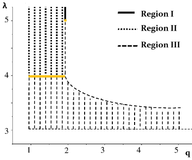
Figure 1: (Color online) Phase diagram of the Potts model on an uncorrelated scale-free network. The area of the second order phase transition is shown. Three regions correspond to three different universality classes. Logarithmic corrections to scaling appear for the values of $q$ and $\lambda$ shown by a light line and a light disc (brown online). See the text for a more detailed discussion.

Figure 1 generalizes the information about the critical behavior of the Potts model on an uncorrelated scale-free network in the form of a phase diagram in the $q-\lambda$ plane [8, 6]. It has been shown that for $\lambda\leqslant 3$, the system remains in the ordered state for any finite temperature [6, 7, 8]. For $\lambda>3$, the phase transition may be of the first or second order, depending on the specific values of $q$ and $\lambda$. The first order phase transition occurs at the values of $q$ and $\lambda$ that belong to the blank region above the dashed curve, $q>2$, $\lambda>\lambda_{\mathrm{c}}(q)$. Of the main interest for us will be the second order phase transition regime. This corresponds to three different regions shown in figure 1 that belong to three different universality classes. Region I, $\lambda>5$, $q=2$ (black solid line in figure 1) is governed by the Ising mean field critical exponents. Region II, $\lambda>4$, $1\leqslant q<2$ (dotted area in the figure) is governed by the percolation mean field critical exponents. Region III ($3<\lambda<5$, $q=2$; $3<\lambda<4$, $1\leqslant q<2$; $3<\lambda\leqslant\lambda_{\mathrm{c}}(q)$, $q>2$) (dashed area in the figure) is characterized by the non-trivial $\lambda$-dependency of the critical exponents. Values of the critical exponents in all three regions are collected in table 1.

Table 1: Critical indices of the Potts model on an uncorrelated scale-free network in three different regions of $q$ and $\lambda$ values, see figure 1. One recovers the results for the Ising model ($q=2$ [30, 31]) and for percolation ($q=1$) [32].

	$\alpha$	$\alpha_{\mathrm{c}}$	$\beta$	$\delta$	$\gamma$	$\gamma_{\mathrm{c}}$	$\omega$	$\omega_{\mathrm{c}}$
region I	0	0	1/2	3	1	2/3	1/2	1/3
region II	$-1$	$-1/2$	1	2	1	1/2	0	0
region III	$\frac{\lambda-5}{\lambda-3}$	$\frac{\lambda-5}{\lambda-2}$	$\frac{1}{\lambda-3}$	$\lambda-2$	$1$	$\frac{\lambda-3}{\lambda-2}$	$\frac{\lambda-4}{\lambda-3}$	$\frac{\lambda-4}{\lambda-2}$

As it was mentioned above, logarithmic terms appear in the free energy at the integer values of $\lambda$. In turn, this leads to the appearance of logarithmic corrections [33, 34, 35] to the power-law scaling dependencies (2.1), (2.2) of thermodynamic functions at $\lambda=5$ for the Ising model ($q=2$) and at $\lambda=4$ for $1\leqslant q<2$ [6]. Values of $q$ and $\lambda$ where the thermodynamic functions are governed by power-law singularities enhanced by the logarithmic corrections are shown in figure 1 by the light solid line and light disc (brown online).

In the forthcoming section we will be interested in the critical behaviour in the regions of the second order phase transition with the power law scaling. In particular, we will complete a quantitative description of three universality classes found in regions I, II and III (see figure 1) by calculating, in addition to the critical exponent, the scaling functions and amplitude ratios.

4 Critical amplitude ratios and scaling functions

The expression of the free energy of the Potts model on an uncorrelated scale-free network (3.3) will be a starting point for the analysis of the critical amplitude ratios and scaling functions. Passing to the dimensionless energy $f(m,\tau)$ and dimensionless magnetization $m$ and leaving the leading order contributions for small values of $m$, we can present (3.3) in three different regions of the phase diagram (figure 1) in the following form:

$$f(m,\tau) =\pm\frac{\tau}{2}m^{2}+\frac{1}{4}m^{4}, \text{(Region I)},$$ (4.1)

$$f(m,\tau) =\pm\frac{\tau}{2}m^{2}+\frac{1}{4}m^{3}, \text{(Region II)},$$ (4.2)

$$f(m,\tau) =\pm\frac{\tau}{2}m^{2}+\frac{1}{4}m^{\lambda-1}, \text{(Region III)},$$ (4.3)

the signs $\pm$ here and in what follows refer to the temperatures above and below the critical point $T_{\mathrm{c}}$. Note that the positive sign of the second terms in (4.1)–(4.3) is due to the fact that coefficients $a_{2}$, $a_{3}$, and $a_{4}$ in (3.3) are positive definite in the regions III, II, and I, correspondingly. With the expressions for the free energy at hand it is straightforward to write down the equation of state and to derive the thermodynamic functions. The magnetic and entropic equations of state in the dimensionless variables $m$ and $\tau$ read:

$$h(m,\tau)=\left.\frac{\partial f(m,\tau)}{\partial m}\right|_{\tau}\,,\qquad s(m,\tau)=\left.\mp\frac{\partial f(m,\tau)}{\partial\tau}\right|_{m}\,.$$ (4.4)

Written explicitly in different regions of $q$, $\lambda$ the magnetic equation of state attains the following form:

$$h =m^{3}\pm\tau m, \text{(Region I)},$$ (4.5)

$$h =\frac{3}{4}m^{2}\pm\tau m, \text{(Region II)},$$ (4.6)

$$h =\frac{\lambda-1}{4}m^{\lambda-2}\pm\tau m, \text{(Region III)}.$$ (4.7)

The entropic equation of state is obtained by a temperature derivative at a constant magnetization $m$ while the explicit $\tau$-dependency is the same in all expressions (4.1)–(4.3). Therefore, the equation keeps the same form in all regions on $q$–$\lambda$ plane:

$$s=-m^{2}/2,\qquad\qquad\text{(Regions I--III)}.$$ (4.8)

Thermodynamic functions $\chi_{T}$, $c_{h}$, and $m_{T}$ that characterize the response on an external action are directly obtained from the above equations of state. We do not present the explicit expressions here, being rather interested in the corresponding critical amplitude ratios. The latter are given in table 2. In the particular case $q=2$, by these expressions we recover the formerly obtained critical amplitude ratios for the Ising model on an uncorrelated scale-free network [36, 23], correcting at $3<\lambda<5$ the expression for $R_{A}$ given in [23]. Together with the previously derived set of critical exponents (see table 1), our results for the critical amplitude ratios quantify the universal features of critical behaviour of the Potts model in the second order phase transition regime.

Table 2: Scaling functions and critical amplitude ratios for the Potts model on an uncorrelated scale-free network.

	Region I	Region II	Region III
$f_{\pm}(x)$	$\pm\frac{x^{2}}{2}+\frac{x^{4}}{4}$	$\pm\frac{x^{2}}{2}+\frac{x^{3}}{4}$	$\pm\frac{x^{2}}{2}+\frac{x^{\lambda-1}}{4}$
$H_{\pm}(x)$	$x^{3}\,\pm\,x$	$\frac{3}{4}x^{2}\,\pm\,x$	$\frac{\lambda-1}{4}x^{\lambda-2}\,\pm\,x$
${\cal S}(x)$	$-x^{2}/2$	$-x^{2}/2$	$-x^{2}/2$
${\cal C_{\pm}}(x)$	$\frac{x^{2}}{3x^{2}\pm 1}$	$\frac{x^{2}}{3x/2\pm\,1}$	$\frac{x^{2}}{(\lambda-1)(\lambda-2)x^{\lambda-3}/4\pm 1}$
$\chi_{\pm}(x)$	$\frac{1}{3x^{2}\,\pm\,1}$	$\frac{1}{3x/2\,\pm\,1}$	$\frac{1}{(\lambda-1)(\lambda-2)x^{\lambda-3}/4\,\pm\,1}$
${\cal M}_{\pm}(x)$	$\frac{x}{3x^{2}\pm 1}$	$\frac{x}{3x/2\pm\,1}$	$\frac{x}{(\lambda-1)(\lambda-2)x^{\lambda-3}/4\pm 1}$
$A^{+}/A^{-}$	$0$	$0$	$0$
$\Gamma^{+}/\Gamma^{-}$	$2$	$1$	$\lambda-3$
$R^{+}_{\chi}$	$1$	$1$	$1$
$R^{-}_{\chi}$	$\frac{1}{2}$	$1$	$\frac{1}{\lambda-3}$
$R^{+}_{\mathrm{c}}$	$0$	$0$	$0$
$R^{-}_{\mathrm{c}}$	$\frac{1}{4}$	$1$	$\frac{1}{(\lambda-3)^{2}}$
$R_{A}$	$\frac{1}{3}$	$\frac{1}{2}$	$\frac{1}{\lambda-2}$

Let us derive now the scaling functions for the free energy and other thermodynamic functions. Using the definition (2.4) and taking into account that the heat capacity and the order parameter critical exponents $\alpha$, $\beta$ take on different values in different regions of the phase diagram figure 1 (the formulas are given in table 1) we can recast Helmholtz potential $F(\tau,m)$ in terms of the scaling function $f_{\pm}(m/\tau^{\beta})$. The explicit expressions for the scaling function in all three regions of the phase diagram are given in table 2. Typical behaviour of the free energy scaling functions $f_{+}(x)$ and $f_{-}(x)$ is shown in figure 2 (a) and 2 (b), correspondingly.

At any value of $q$, the scaling functions share a common feature: their curvature gradually increases with an increase of $\lambda>3$. This happens up to some marginal value $\lambda=\lambda_{\mathrm{c}}$. The marginal value $\lambda_{\mathrm{c}}$ is $q$-dependent. For $\lambda>\lambda_{\mathrm{c}}$ and $1\leqslant q\leqslant 2$, the scaling functions remain unchanged: their shape does not change with a further increase of $\lambda$. The logarithmic corrections to scaling appear at $\lambda=\lambda_{\mathrm{c}}$ and the second order phase transition holds in this case for $\lambda>\lambda_{\mathrm{c}}$ as well [6], see figure 1. Alternatively, for $\lambda>\lambda_{\mathrm{c}}$ and $q>2$, the phase transition turns out to be of the first order. Curves I of figure 2 (plotted by solid lines) show the limiting behaviour of the scaling functions at $q=2$, $\lambda>5$ [note that $\lambda_{\mathrm{c}}(q=2)=5$]: the functions remain unchanged for all $\lambda>5$. Similar behaviour holds for the case $1\leqslant q<2$, the value of $\lambda_{\mathrm{c}}$, however, differs: $\lambda_{\mathrm{c}}(1\leqslant q<2)=4$. This is shown by curves II in the figure, plotted by dashed lines. Finally, curves III (dotted lines) for $q=4$ are one of examples of the limiting behaviour of the scaling functions in the region $q>2$.

         

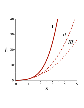
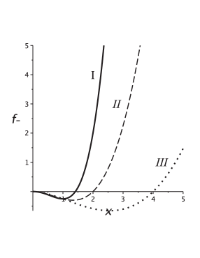
       (a)                                                      (b)

Figure 2: (Color online) Limiting behaviour of the free energy scaling functions $f_{+}$ [(a), $T>T_{\mathrm{c}}$] and $f_{-}$ [(b), $T<T_{\mathrm{c}}$]. The functions remain unchanged for $\lambda>5$, $q=2$ and $\lambda>4$, $1\leqslant q<2$ (solid and dashed curves I and II, correspondingly). For $q>2$ the phase transition turns out to be of the first order at $\lambda>\lambda_{\mathrm{c}}(q)$. Dotted curves III: $q=4$, $\lambda=\lambda_{\mathrm{c}}(4)\simeq 3.5$. See the text for more details.

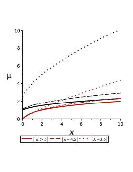
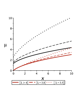
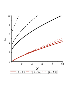
     (a)                                               (b)                                               (c)

Figure 3: (Color online) Behaviour of the order parameter scaling functions $\mu_{+}(x)$ (light curves, brown online) and $\mu_{-}(x)$ (black curves) for different values of $\lambda$ and $q$. (a): $q=2$, (b): $1\leqslant q<2$, (c): $q=4$. Values of $\lambda$ are shown in the figures.

Entropy scaling function ${\cal S}(x)$ is defined by (2.6). Using expression (4.8) for the entropy and taking into account the values for the critical exponents $\alpha$ and $\beta$ given in table 1 we arrive at the entropy scaling function that remains unchanged in all regions on $q$–$\lambda$ plane: ${\cal S}(x)=-x^{2}/2$. There are different ways of representing the magnetic equation of state. In the Widom-Griffiths representation [37, 38] the magnetic equation of state can be written in two equivalent forms:

$$h=m^{\delta}h_{\pm}\left(\tau/m^{1/\beta}\right)\,,\qquad h=\tau^{\beta\delta}H_{\pm}\left(m/\tau^{\beta}\right)\,,$$ (4.9)

with scaling functions $h_{\pm}(x)$ and $H_{\pm}(x)$. Alternatively, in Hankey-Stanley representation, the magnetization is written as [25]:

$$m=\tau^{\beta}\mu_{\pm}\left(h/\tau^{\beta\delta}\right)\,$$ (4.10)

with the scaling function $\mu_{\pm}(x)$.

Starting from the magnetic equation of state given in regions I–III by equations (4.5)–(4.7), it is straightforward to arrive at the scaling functions $H_{\pm}(x)$. We give the appropriate expressions in table 2. Subsequently, one can easily rewrite these expressions to get appropriate $h_{\pm}$-functions. Behaviour of the scaling functions $\mu_{\pm}(x)$ for different values of $\lambda$ and $q$ is shown in figure 3. From the explicit form of the equation of state it is easy to evaluate the asymptotic behaviour of the scaling functions. For $q=2$ and $\lambda>5$, one gets $\mu_{\pm}(x)\sim x^{1/3},\,x\to\infty$. The functions tend to turn to infinity faster with a decrease of $\lambda$: $\mu_{\pm}(x)\sim x^{1/(\lambda-2)},\,x\to\infty$ for $3<\lambda<5$. A similar feature is observed for the other values of $q$. At $1\leqslant q<2$, $\lambda>4$ one gets $\mu_{\pm}(x)\sim\sqrt{x},\,x\to\infty$ and $\mu_{\pm}(x)\sim x^{1/(\lambda-2)},\,x\to\infty$ for $3<\lambda<4$. The last asymptotic behaviour also holds for $q>2$ and $\lambda\leqslant\lambda_{\mathrm{c}}(q)$. Note that all light curves (brown online) in figure 3 start form the origin: this corresponds to the absence of spontaneous magnetization at $T>T_{\mathrm{c}}$. Correspondingly, the value of the scaling function $\mu_{-}(x)$ at $x=0$ gives the spontaneous magnetization critical amplitude $B_{-}$, equation (2.2). As one can see in figure 3, the latter increases with a decrease of $\lambda$.

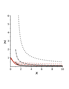
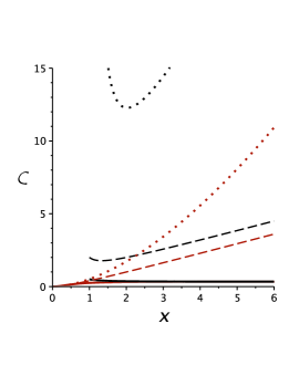
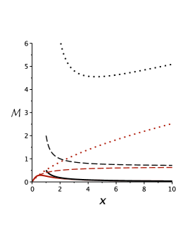
     (a)                                               (b)                                               (c)

Figure 4: (Color online) Scaling functions for the isothermal susceptibility (a), heat capacity (b), and magnetocaloric coefficient (c). Light curves, brown online, $T>T_{\mathrm{c}}$: $\chi_{+}(x)$, ${\cal C_{+}}(x)$, ${\cal M_{+}}(x)$. Black curves, $T<T_{\mathrm{c}}$: $\chi_{-}(x)$, ${\cal C_{-}}(x)$, ${\cal M_{-}}(x)$. Solid, dashed and dotted curves correspond to the values of $q$ and $\lambda$ of the free energy scaling functions of figure 2.

In figures 4 we show the behaviour of the scaling functions for thermodynamic observables that characterize the response of a system to an external action, i.e., the isothermal susceptibility [figure 4 (a)], heat capacity [figure 4 (b)], and magnetocaloric coefficient [figure 4 (c)]. The values of $q$ and $\lambda$, for which the curves are plotted are the same as those for the free energy scaling functions in figure 2: they reflect the limiting behaviour at some marginal value $\lambda_{\mathrm{c}}(q)$. At $1\leqslant q\leqslant 2$ and $\lambda>\lambda_{\mathrm{c}}(q)$, the phase transition remains the second order but the critical exponents do not depend on $\lambda$ any more, the scaling function does not depend on $\lambda$ either. However, for $q>2$, $\lambda>\lambda_{\mathrm{c}}(q)$, the phase transition turns to the first order and the scaling regime does not hold any more. In turn, in the region below $\lambda_{\mathrm{c}}$, the exponents acquire $\lambda$-dependency, so do the scaling functions, as is plotted in the figures.

5 Conclusions

In this paper we were interested in an analysis of the critical behaviour of the Potts model on uncorrelated scale-free network. In our previous work the list of critical exponents for the Potts model in the second order phase transition regime was obtained [6]. Here, we complete quantitative characteristics of the universal features by calculation of the amplitude ratios and scaling functions. Our results are exact for the annealed scale-free network and correspond to the mean field treatment of the quenched case.

We obtain general scaling functions for the order parameter, entropy, the constant-field heat capacity, magnetic susceptibility and the isothermal magnetocaloric coefficient near the critical point. The comprehensive list of scaling functions and critical amplitude ratios was obtained in different regions of $q$ and $\lambda$. It was shown that the critical amplitude ratios are $\lambda$-dependent similar to the critical exponents, so $\lambda$ plays the role of a global parameter of the system.

Ukrainian 0

Скейлiнговi функцiї та спiввiдношення амплiтуд для моделi Поттса на нескорельованiй безмасштабнiй мережi М. Красницька${}^{\textsf{\footnotesize{\mbox{?},\penalty 1000\mbox{?}}}}$

             
${}^{\textsf{\footnotesize 1}}$ Iнститут фiзики конденсованих систем НАН України, вул. I. Свєнцiцького, 1, 79011 Львiв, Україна ${}^{\textsf{\footnotesize 2}}$ Iнститут Жаня Лямура, CNRS/UMR 7198, Група статистичної фiзики, Унiверситет Лотарингiї,
BP 70239, F-54506 Вандувр лє-Нансi, Францiя

References

- [1] Fisher M.E., Rep. Prog. Phys., 1967, 30, 615; doi:10.1088/0034-4885/30/2/306.
- [2] Kadanoff L., Götze W., Hamblen D., Hecht R., Lewis E.A.S., Palciauskas V.V., Rayl M., Swift J., Aspnes D., Kane J., Rev. Mod. Phys., 1967, 39, 395; doi:10.1103/RevModPhys.39.395.
- [3] Domb C., The critical point, Taylor & Francis, London, 1996.
- [4] Privman V., Hohenberg P.C., Aharony A., In: Phase Transitions and Critical Phenomena, Vol. 14, Domb C., Lebowitz J.L. (Eds.), Academic Press, New York, 1991.
- [5] Dorogovtsev S.N., Goltsev A.V., Mendes J.F.F., Rev. Mod. Phys., 2008, 80, 1275; doi:10.1103/RevModPhys.80.1275.
- [6] Krasnytska M., Berche B., Holovatch Yu., Condens. Matter Phys., 2013, 16, 23602; doi:10.5488/CMP.16.23602.
- [7] Dorogovtsev S., Goltsev A.V., Mendes J.F.F., Eur. Phys. J. B, 2004, 38, 177; doi:10.1140/epjb/e2004-00019-y.
- [8] Iglói F., Turban L., Phys. Rev. E, 2002, 66, 036140; doi:10.1103/PhysRevE.66.036140.
- [9] Kasteleyn P.W., Fortuin C.M., J. Phys. Soc. Jpn. (Suppl.), 1969, 26, 11.
- [10] Giri M.R., Stephen M.J., Grest G.S., Phys. Rev. B, 1977, 16, 4971; doi:10.1103/PhysRevB.16.4971.
- [11] Stephen M.J., Phys. Lett. A, 1976, 56, 149; doi:10.1016/0375-9601(76)90625-3.
- [12] Fortiun C.M., Kasteleyn P.W., Physica, 1972, 57, 536; doi:10.1016/0031-8914(72)90045-6.
- [13] Majumdar S.N., Dhar D., Physica A, 1992, 185, 129; doi:10.1016/0378-4371(92)90447-X.
- [14] Aharony A., J. Phys. C: Solid State Phys., 1978, 11, L457; doi:10.1088/0022-3719/11/11/004.
- [15] Aharony A., Pfeuty P., J. Phys. C: Solid State Phys., 1979, 12, L125; doi:10.1088/0022-3719/12/3/008.
- [16] Lubensky T.C., Isaacson J., Phys. Rev. Lett., 1978, 41, 12; doi:10.1103/PhysRevLett.41.829.
- [17] Mukamel D., Fisher M.E., Domany E., Phys. Rev. Lett., 1976, 37, 10; doi:10.1103/PhysRevLett.37.565.
- [18] Alexander S., Phys. Lett. A, 1975, 54, 353; doi:10.1016/0375-9601(75)90766-5.
- [19] Bretz M., Phys. Rev. Lett., 1977, 38, 9; doi:10.1103/PhysRevLett.38.501.
- [20] Domany E., Schick M., Walker J.S., Phys. Rev. Lett., 1977, 38, 1148; doi:10.1103/PhysRevLett.38.1148.
- [21] Turner S., Sherratt J.A., J. Theor. Biol., 2002, 216, 85; doi:10.1006/jtbi.2001.2522.
-
[22]
Laanait L., Messager A., Miracle-Sole S.,
Ruiz J., Shlosman S., Commun. Math. Phys., 1991, 140, 81;
doi:10.1007/BF02099291. -
[23]
Von Ferber C., Folk R., Holovatch Yu., Kenna R., Palchykov V., Phys. Rev. E, 2011, 83, 061114;
doi:10.1103/PhysRevE.83.061114. - [24] Stanley H.E., Rev. Mod. Phys., 1999, 71, S358; doi:10.1103/RevModPhys.71.S358.
- [25] Hankey A., Stanley H.E., Phys. Rev. B, 1972, 6, 3515; doi:10.1103/PhysRevB.6.3515.
- [26] Wu F.Y., Rev. Mod. Phys., 1982, 54, 235; doi:10.1103/RevModPhys.54.235.
- [27] Lee S.H., Ha M., Jeong H., Noh J.D., Park H., Phys. Rev. E, 2009, 80, 051127; doi:10.1103/PhysRevE.80.051127.
- [28] Bianconi G., Phys. Rev. E, 2012, 85, 061113; doi:10.1103/PhysRevE.85.061113.
- [29] Dorogovtsev S.N., Goltsev A.V., Mendes J.F.F., Phys. Rev. E, 2002, 66, 016104; doi:10.1103/PhysRevE.66.016104.
- [30] Leone M., Vázquez A., Vespignani A., Zecchina R., Eur. Phys. J. B, 2002, 28, 191; doi:10.1140/epjb/e2002-00220-0.
- [31] Goltsev A.V., Dorogovtsev S., Mendes J.F.F., Phys. Rev. E, 2003, 67, 026123; doi:10.1103/PhysRevE.67.026123.
- [32] Cohen R., ben-Avraham D., Havlin S., Phys. Rev. E, 2002, 66, 036113; doi:10.1103/PhysRevE.66.036113.
- [33] Kenna R., Johnston D.A., Janke W., Phys. Rev. Lett., 2006, 96, 115701; doi:10.1103/PhysRevLett.96.115701.
- [34] Kenna R., Johnston D.A., Janke W., Phys. Rev. Lett., 2006, 97, 155702; doi:10.1103/PhysRevLett.97.155702.
- [35] Berche B., Butera P., Shchur L., J. Phys. A: Math. Theor., 2013, 46, 095001; doi:10.1088/1751-8113/46/9/095001.
-
[36]
Palchykov V., von Ferber C., Folk R., Holovatch Yu., Kenna R., Phys. Rev. E, 2010, 82, 011145;
doi:10.1103/PhysRevE.82.011145. - [37] Griffiths R.B., Phys. Rev., 1967, 158, 176; doi:10.1103/PhysRev.158.176.
- [38] Widom B., J. Chem. Phys., 1965, 43, 3898; doi:10.1063/1.1696618.
Ukrainian \adddialect\l@ukrainian0 \l@ukrainian