Abstract

A symmetry $SU(2,2)$ group in terms of ladder operators is presented for the Jacobi polynomials, $J_{n}^{({\alpha},\beta)}(x)$, and the Wigner $d_{j}$-matrices where the spins $j=n+({\alpha}+\beta)/2$ integer and half-integer are considered together. A unitary irreducible representation of $SU(2,2)$ is constructed and subgroups of physical interest are discussed.

The Universal Enveloping Algebra of $su(2,2)$ also allows to construct group structures ($SU(1,1)$, $SO(3,2)$, $Spin(3,2)$) whose representations separate integers and half-integers values of the spin $j$.

Appropriate $L^{2}$–functions spaces are realized inside the support spaces of all these representations. Operators acting on these $L^{2}$–functions spaces belong thus to the corresponding Universal Enveloping Algebra.

Keywords: Special functions, Jacobi polynomials, Wigner $d_{j}$-matrices, Lie algebras, Square-integrable functions

1 Introduction

Many attempts have been done to find a wide but not too inclusive class of functions that can be defined “special”, where “special” means something more that “useful” [1].

The actual main line of work for a possible unified theory of special functions is the Askey scheme that is based on the analytical theory of linear differential equations [2, 3, 4].

However, a possible alternative point of view was established by employing considerations that belong to a field of mathematics seemingly quite far from them: the theory of representations of Lie groups. This way was introduced by Wigner [5] and Talman [6] and later developed mainly by Miller [7] and Vilenkin and Klimyk [8, 9, 10]. In this line, previous papers by us shown a direct connection between some special functions and well defined Lie groups. The starting point of our work has been the paradigmatic example of Hermite functions that are a basis on the Hilbert space of the square integrable functions defined on the configuration space ${\mathbb{R}}$. As it is well known in the algebraic discussion of the harmonic oscillator, besides the configuration basis, $\{|x\rangle\}_{x\in{\mathbb{R}}}$ , a discrete basis, $\{|n\rangle\}_{n\in{\mathbb{N}}}$ – related to the Weyl-Heisenberg group $H(1)$ – can be introduced such that Hermite functions are the transition matrices from one basis to the other. This scheme has been generalized to all the orthogonal polynomials we have, up to now, considered: Legendre and Laguerre polynomials [11], associated Legendre polynomials and Spherical Harmonics [12]. We discuss here the Lie group properties of Jacobi polynomials and Wigner $d_{j}$-matrices.

Starting from the seminal work by Truesdell [13], where a sub-class of special functions is defined by means of a set of formal properties, we proposed a possible definition of a fundamental sub-class of special functions, called “algebraic special functions” (ASF). These ASF look to be strictly related to the hypergeometric functions but are constructed from the following algebraic assumptions:

1. A set of differential recurrence relations exists on these ASF that can be associated to a set of ladder operators that span a Lie algebra.

2. These ASF support an irreducible representation of this algebra.

3. A Hilbert space can be constructed on these ASF where the ladder operators have the hermiticity properties appropriate for constructing a unitary irreducible representation (UIR) of the associated Lie group.

4. Second order differential equation that define the ASF can be reconstructed from all diagonal elements of the Universal Enveloping Algebra (UEA) and, in particular, from the second order Casimirs of all subalgebras and of the whole algebra.

From these assumptions, we have that:

• Applying the exponential map to ASF different sets of functions can be constructed. If the transformation is unitary another algebraically equivalent basis of the Hilbert space is obtained. When the transformations are not unitary, as in the case of coherent states, sets with different properties are found (like overcomplete sets).

• The ASF are also a basis of an appropriate set of $L^{2}$–functions and of an appropriate Hilbert space functions. This, combined with the above properties, implies that the vector space of the operators operating on $L^{2}$ (or Hilbert) space functions is homomorphic to the UEA built on the algebra.

In [11] it has been shown that Hermite, Laguerre and Legendre polynomials are ASF such that the Hermite functions support a UIR of the Weyl-Heisenberg group $H(1)$ with Casimir ${\cal C}=0$, while Laguerre functions and Legendre polynomials are both bases for the UIR of $SU(1,1)$ with ${\cal C}=-1/4$. Since Hermite functions are a basis of square-integrable functions defined on the real line, as well as Laguerre functions on the semi-line and Legendre polynomials on the finite interval [14], all operators acting on such $L^{2}$–functions can be written inside the universal enveloping algebra (UEA) of $h(1)$ or $su(1,1)$. All these properties have been shown to not be restricted to the above mentioned 1-rank algebras (and groups). Indeed in [12] Associated Legendre polynomials and Spherical Harmonics are shown to share the same properties with underlying Lie group $SO(3,2)$ that is of rank 2 like two, ${l}$ and ${m}$, are the label parameters of these functions.

Here we present a further confirmation of this scheme in terms of the Jacobi polynomials and Wigner $d_{j}$-matrices showing that they satisfy the required conditions to be considered ASF and share the same properties. Indeed they can be associated to well defined “algebraic Jacobi functions” (AJF) that support a UIR of $SU(2,2)$ i.e., a Lie group of rank 3 like three are the parameters, $(n,\alpha,\beta)$, of the Jacobi polynomials $J_{n}^{({\alpha},\beta)}(x)$ and three $(j,m,q)$ are also the ones of $d^{j}_{q,m}$ matrices.

From an applied point of view for both, AJF and Wigner $d_{j}$–matrices, the relevant group chains are $SU(2,2)\supset SU(2)\otimes SU(2)\supset SU(2)$ to consider together integer and half-integer spin $j$ and $SU(2,2)\supset SU(1,1)$ to describe them separately.

The paper is organized as follows. Section 2 is devoted to present the main properties of the AJF relevant for our discussion and their relations with the Wigner $d_{j}$-matrices. In section 3 we study the symmetries of the AJF that keep invariant the principal parameter $j$ and change $m$ and/or $q$. We prove that these ladder operators determine a $su(2)\oplus su(2)$ algebra, that allows us to build up a family of UIR of the group $SU(2)\otimes SU(2)$, i.e. $U^{j}\otimes U^{j}$. In section 4 we construct, by means of four new sets of ladder operators that change the three parameters $j,m$ and $q$ in $\pm 1/2$, each of them generating a $su(1,1)$ algebra to which infinitely many UIR’s of $SU(1,1)$ – supported by the AJF – are associated. In Sect. 5 we show that the ladder operators, obtained in previous sections, span a $su(2,2)$ Lie algebra and the AJF and Wigner $d_{j}$-matrices generate a UIR of $SU(2,2)$ characterized by the eigenvalue of the quadratic Casimir ${\cal C}_{SU(2,2)}=-3/2$. Next Section shows the AJF and Wigner $d_{j}$–matrices with labels all integers and half-integers can be classified in different and disconnected UIR representations of $SU(1,1)$ or $SO(3,2)$. In section 7 the homomorphism between the space of the operators on the $L^{2}$ space and the UEA of $su(2,2)$ is discussed. Finally some conclusions and comments are included.

A previous unpublished version of this work containing part of the results here presented can be found in [15].

2 Algebraic Jacobi functions and their operatorial structure

We consider the Jacobi polynomials, $J_{n}^{({\alpha},\beta)}(x)$, of degree $n\in{\mathbb{N}}$ as defined in terms of the hypergeometric functions  ${}_{2}F_{1}$ [16, 17] by

$$J_{n}^{({\alpha},\beta)}(x)=\;\frac{({\alpha}+1)_{n}}{n!}\;\;\;_{2}F_{1}\left[-n,1+{\alpha}+\beta+n;{\alpha}+1;\frac{1-x}{2}\right],$$ (2.1)

where $(a)_{n}:=a\,(a+1)\cdots(a+n-1)$ is the Pochhammer symbol, or equivalently by [18]

$$J_{n}^{({\alpha},\beta)}(x)=\;\frac{({\alpha}+1)_{n}}{n!}\;\left(\frac{1+x}{2}\right)^{n}\;\;_{2}F_{1}\left[-n,-n-\beta;{\alpha}+1;\frac{x-1}{x+1}\right].$$ (2.2)

From (2.2) an explicit polynomial expression can be obtained [19]

$$J_{n}^{({\alpha},\beta)}(x)=\;\sum_{s=0}^{n}\;\left(\begin{array}[]{c}n+{\alpha}\\ s\end{array}\right)\;\left(\begin{array}[]{c}n+\beta\\ n-s\end{array}\right)\;\left(\frac{x+1}{2}\right)^{s}\;\left(\frac{x-1}{2}\right)^{n-s}\;\;.$$ (2.3)

where we have considered a generalized binomial coefficient

$$\left(\begin{array}[]{c}a\\ s\end{array}\right):=\frac{(a+1-s)_{s}}{s!},$$

being $a$ an arbitrary number and $s$ a positive integer.

However to obtain objects related to an algebraic structure like in [11, 12], we define -alternatively to $n,{\alpha},\beta$- three other (discrete) variables and include an $x$-depending factor. We first substitute $(n,{\alpha},\beta)$ with $(j,m,q)$

$$j:=n+\frac{{\alpha}+\beta}{2}\,,\qquad m:=\frac{{\alpha}+\beta}{2}\,,\qquad q:=\frac{{\alpha}-\beta}{2}\,,$$

hence

$$n=j-m,\qquad{\alpha}=m+q,\qquad\beta=m-q\;.$$

Then, in a second and final step, we include a $x$-depending factor related with the integration measure of the Jacobi polynomials. So, the fundamental objects of this paper, we call “algebraic Jacobi functions” (AJF), have the final form

$${\cal J}_{j}^{m,q}(x):=\sqrt{\frac{\Gamma(j+m+1)\,\Gamma(j-m+1)}{\Gamma(j+q+1)\,\Gamma(j-q+1)}}\,\left(\frac{1-x}{2}\right)^{\frac{m+q}{2}}\,\left(\frac{1+x}{2}\right)^{\frac{m-q}{2}}\,J_{j-m}^{(m+q,m-q)}(x),$$ (2.4)

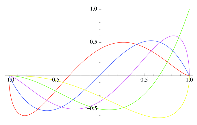
Figure 1: ${\cal J}_{3}^{2,1}$ (red), ${\cal J}_{3}^{2,0}$ (blue), ${\cal J}_{3}^{2,-1}$ (magenta), ${\cal J}_{3}^{2,-2}$ (green), ${\cal J}_{3}^{2,-3}$ (yellow).

where in order to obtain a group representation, as we will prove later, we have to impose the following restrictions for $(j,m,q)$

$$j\geq|m|,\qquad j\geq|q|,\qquad 2j\in{\mathbb{N}},\quad j-m\in{\mathbb{N}},\;\;j-q\in{\mathbb{N}}$$ (2.5)

Hence, $(j,m,q)$ are all together integers or half-integers (see Fig. 1 and Fig. 2 where some AFS for different integers and half-integers values of $(j,m,q)$ are displayed).

The conditions (2.5) rewritten in terms of the original parameters $(n,{\alpha},\beta)$ are

$$n\in{\mathbb{N}},\qquad{\alpha},\beta\in{\mathbb{Z}},\qquad{\alpha}\geq-n,\qquad\beta\geq-n,\qquad{\alpha}+\beta\geq-n.$$

Note that usually the Jacobi polynomials $J_{n}^{({\alpha},\beta)}(x)$ are defined for ${\alpha}>-1$ and $\beta>-1$ (${\alpha},\,\beta\in{\mathbb{R}}$) in such a way that a unique weight function $w(x)$ allows their normalization. However (see also [19] p. 49) we have to change such restrictions since we introduce the normalization inside the functions and the algebra requires eq. (2.5). In principle -because from the definition (2.4) ${\cal J}_{j}^{m,q}(x)=0$ for $j<|q|$- the AJF could be extended to $j<|m|$ considering

$$\hat{\cal J}_{j}^{m,q}(x):=\lim_{\varepsilon\to 0}{\cal J}_{j}^{m+\varepsilon,q}(x)$$

as

$$\hat{\cal J}_{j}^{m,q}(x)=\left\{\begin{array}[]{cl}{\cal J}_{j}^{m,q}(x)&\forall\,(j,m,q)\;\;\text{verifying all conditions \eqref{conditions}}\\[8.5359pt] 0&{j<|m|}\end{array}\right..$$

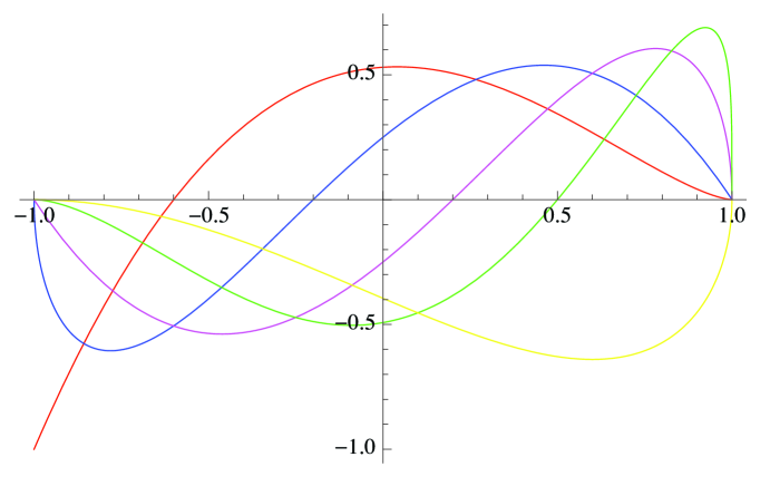
Figure 2: ${\cal J}_{\frac{5}{2}}^{\frac{3}{2},\frac{3}{2}}$ (red), ${\cal J}_{\frac{5}{2}}^{\frac{3}{2},\frac{1}{2}}$ (blue), ${\cal J}_{\frac{5}{2}}^{\frac{3}{2},-\frac{1}{2}}$ (magenta), ${\cal J}_{\frac{5}{2}}^{\frac{3}{2},-\frac{3}{2}}$ (green), ${\cal J}_{\frac{5}{2}}^{\frac{3}{2},-\frac{5}{2}}$ (yellow).

The AJF (2.4) reveal additional symmetries hidden inside the Jacobi polynomials. Indeed we have

$$\begin{array}[]{lll}{\cal J}_{j}^{m,q}(x)={\cal J}_{j}^{q,m}(x),\\[8.5359pt] {\cal J}_{j}^{m,q}(x)=(-1)^{l-m}\,{\cal J}_{j}^{m,-q}(-x),\\[8.5359pt] {\cal J}_{j}^{m,q}(x)=(-1)^{l-q}\,{\cal J}_{j}^{-m,q}(-x),\\[8.5359pt] {\cal J}_{j}^{m,q}(x)=(-1)^{m+q}\,{\cal J}_{j}^{-m,-q}(x)\,.\end{array}$$ (2.6)

The proof of these properties is straightforward. The first one can be proved taking into account the following property of the Jacobi polynomials for integer coefficients $(n,{\alpha},\beta)$ [19]

$$\begin{array}[]{lll}{J}_{n}^{{\alpha},\beta}(x)=\displaystyle{\frac{(n+{\alpha})!\,(n+\beta)!}{n!\,(n+{\alpha}+\beta)!}}\,\left(\frac{x+1}{2}\right)^{-\beta}\,{J}_{n+\beta}^{{\alpha},-\beta}(x)\,.\end{array}$$

The second property can be derived from the well-known symmetry of the Jacobi polynomials [16]

$$J_{n}^{({\alpha},\beta)}(x)=(-1)^{n}J_{n}^{(\beta,{\alpha})}(-x),$$

and the last two properties can be proved using the first two ones.

These AJF for $m$ and $q$ fixed verify the orthogonality relation

$$\int_{-1}^{1}\,{\cal J}_{j}^{m,q}(x)\;(j+1/2)\;{\cal J}_{j^{\prime}}^{m,q}(x)\,dx=\delta_{j\,j^{\prime}}$$ (2.7)

as well as

$$\sum_{j={\it sup}(|m|,|q|)}^{\infty}{\cal J}_{j}^{m,q}(x)\;\left(j+1/2\right)\;{\cal J}_{j}^{m,q}(y)=\delta(x-y).$$ (2.8)

Both relations are similar to those of the Legendre polynomials [11] and the associated Legendre polynomials [12]: all are orthonormal only up to the factor $j+1/2$.

The Jacobi equation

$$\left[(1-x^{2})\frac{d^{2}}{dx^{2}}-(({\alpha}+\beta+2)x+({\alpha}-\beta))\frac{d}{dx}+n(n+{\alpha}+\beta+1)\right]\,J_{n}^{({\alpha},\beta)}(x)=0$$

rewritten in terms of these new functions ${\cal J}_{j}^{m,q}(x)$ and of the new parameters $(j,m,q)$ becomes

$$\left[-(1-x^{2})\,\frac{d^{2}}{dx^{2}}+2\,x\frac{d}{dx}+\frac{2\;m\;q\;x+m^{2}+q^{2}}{1-x^{2}}-j(j+1)\right]\,{\cal J}_{j}^{m,q}(x)=0\;,$$ (2.9)

where the symmetry under the interchange $m\Leftrightarrow q$ is evident.

It is worthy noticing that the AJFs (2.4), with the substitution $x=\cos\beta$, are essentially the elements of the Wigner $d_{j}$ rotation matrices [20, 19]

$$d^{j}_{qm}(\beta)=\sqrt{\frac{(j+m)!\,(j-m)!}{(j+q)!\,(j-q)!}}\,(\sin\beta/2)^{m-q}\,(\cos\beta/2)^{m+q}\,J^{(m-q,m+q)}_{j-m}(\cos\beta)$$

that verify the conditions (2.5). The explicit relation between them is

$$d^{j}_{qm}(\beta)={\cal J}^{m,-q}_{j}(\cos\beta).$$ (2.10)

Eqs. (2.6) are equivalent to the well-known relations among the $d^{j}_{qm}$ like, for instance,

$$d^{j}_{qm}(\beta)=(-1)^{q-m}\,d^{j}_{mq}(\beta).$$

The paper could be rewritten in terms of the $d^{j}_{qm}$ but the formal complexity should be larger and, perhaps, this is the reason why the lying algebras were not known up to now.

Coming back to the AJF, the starting point for finding the algebra is now the construction of the rising/lowering differential operators that change the labels $(j,m,q)$ of the AJF by 1 or 1/2. The fundamental limitation of this analytical approach is that the indices are considered as parameters [7] that, in iterated applications, must be introduced by hand. This problem has been solved in [11] where a consistent vector space framework was introduced to allow the iterated use of recurrence formulas by means of operators of which the parameters involved are eigenvalues.

Indeed – in order to display the operator structure on the set $\{{\cal J}_{j}^{m,q}(x)\}$ – we introduce, in consistency with the quantum theory approach, not only the operators $X$ and $D_{x}$ of the configuration space, such that

$$X\,f(x)=x\,f(x),\qquad D_{x}\,f(x)=f^{\prime}(x),\qquad[X,D_{x}]=-1\,,$$

but also three other operators $J$, $M$ and $Q$ such that

$$J\;{\cal J}_{j}^{m,q}(x)=j\;{\cal J}_{j}^{m,q}(x)\quad\;M\,{\cal J}_{j}^{m,q}(x)=\,m\;{\cal J}_{j}^{m,q}(x)\,\quad\;Q\,{\cal J}_{j}^{m,q}(x)=\,q\;{\cal J}_{j}^{m,q}(x),$$ (2.11)

i.e. diagonal on the algebraic Jacobi functions and, thus, belonging -in the whole algebraic scheme- to the Cartan subalgebra.

3 Algebras for Jacobi functions with $\Delta j=0$

We start from the differential-difference equations and the difference equations verified by the Jacobi functions (a complete list of which can be found in Refs. [16, 17, 18]). The procedure is laborious, so that, we only sketch the simplest case with $\Delta j=0$, related with $su(2)$ and well-known for the $d_{j}$ in terms of the angle [21].

Let us start from the operators that change the values of $m$ only. Consider the equations (18.9.15) and (18.9.16) of Ref. [16]

$$\begin{array}[]{rll}\displaystyle\frac{d}{dx}J_{n}^{(\alpha,\beta)}(x)&=&\displaystyle\frac{1}{2}(n+\alpha+\beta+1)\,J_{n-1}^{(\alpha+1,\beta+1)}(x)\;,\\[8.5359pt] \displaystyle\frac{d}{dx}\left[(1-x)^{\alpha}(1+x)^{\beta}J_{n}^{(\alpha,\beta)}(x)\right]&=&\displaystyle-2(n+1)(1-x)^{\alpha-1}(1+x)^{\beta-1}\,J_{n+1}^{(\alpha-1,\beta-1)}(x),\end{array}$$

which are far to be symmetric, but allow us to define the operators

$$A_{\pm}:=\;\pm\,\sqrt{1-X^{2}}\,D_{x}\,+\,\frac{1}{\sqrt{1-X^{2}}}\;(XM+Q),$$ (3.1)

that act on the algebraic Jacobi functions ${\cal J}_{j}^{m,q}(x)$ as

$$A_{\pm}\;{\cal J}_{j}^{m,q}(x)=\sqrt{(j\mp m)\,(j\pm m+1})\;\,{\cal J}_{j}^{m\pm 1,\,q}(x).$$ (3.2)

The operators (3.1) are a generalization for $Q\neq 0$ of the operators $J_{\pm}$ introduced in Ref. [12] for the associated Legendre functions related to the AJF with $q=0$. Moreover eqs. (3.2), that are independent from $q$, coincide with eqs. (2.11) and (2.12) of Ref. [12].

Defining now $A_{3}:=M$ and taking into account the action of the operators $A_{\pm}$ and $A_{3}$ on the Jacobi functions, eqs. (3.2) and (2.11), it is easy to check that $A_{\pm}$ and $A_{3}$ close a $su(2)$ algebra, that commutes with $J$ and $Q$, denoted in the following by $su_{A}(2)$

$$[A_{3},A_{\pm}]=\pm A_{\pm}\qquad[A_{+},A_{-}]=2A_{3}.$$

Thus, the algebraic Jacobi functions $\{{\cal J}_{j}^{m,q}(x)\}$ such that $2j\in{\mathbb{N}}$, $j-m\in{\mathbb{N}}$ and $-j\leq m\leq j$ support the $(2j+1)$-dimensional UIR of the Lie group $SU_{A}(2)$ independently from the value of $q$.

Similarly to [12], starting from the differential realization (3.1) of the $A_{\pm}$ operators we recover the Jacobi differential equation (2.9) from the Casimir, ${\cal C}_{A}$, of $su_{A}(2)$

$$\left[{\cal C}_{A}-J(J+1)\right]\;{\cal J}_{j}^{m,q}(x)\equiv\left[A_{3}^{2}+\frac{1}{2}\{A_{+},A_{-}\}-J(J+1)\right]\,{\cal J}_{j}^{m,q}(x)=0\;.$$ (3.3)

Indeed, eq. (3.3) reproduces the operatorial form of (2.9), i.e.

$$\left[-(1-X^{2})D^{2}_{x}+2XD_{x}+\frac{1}{1-X^{2}}(2XMQ+M^{2}+Q^{2})-J(J+1)\right]{\cal J}_{j}^{m,q}(x)=0.$$ (3.4)

On the other hand we can make use of the factorization method [22, 23], relating second order differential equations to product of first order ladder operators in such a way that the application of the first operator modifies the values of the parameters of the second one. Taking into account this fact, iterated application of (3.1) gives the two equations

$$\begin{array}[]{l}\left[A_{+}\,A_{-}-(J+M)\,(J-M+1)\right]\;{\cal J}_{j}^{m,q}(x)=0\;,\\[8.5359pt] \left[A_{-}\,A_{+}-(J-M)\,(J+M+1)\right]\;{\cal J}_{j}^{m,q}(x)=0\;,\end{array}$$ (3.5)

that reproduce again the operator form (3.4) of the Jacobi equation. Equations (3.3), (3.5) are particular cases of a general rule: the defining Jacobi equation can be recovered appliying to ${\cal J}_{j}^{m,q}$ the Casimir operator of any involved algebra and sub-algebra as well as any diagonal product of ladder operators.

Now, using the symmetry $m\Leftrightarrow q$ of the ${\cal J}_{j}^{m,q}(x)$, we construct the algebra that changes $q$ leaving $j$ and $m$ unchanged. From $A_{\pm}$ two new operators $B_{\pm}$ are thus defined

$$B_{\pm}:=\pm\,\sqrt{1-X^{2}}\,D_{x}+\frac{1}{\sqrt{1-X^{2}}}\,(XQ+M)\,,$$ (3.6)

and their action on the Jacobi functions is

$$B_{\pm}\,{\cal J}_{j}^{m,n}(x)=\sqrt{(j\mp q)\,(j\pm q+1})\;\,{\cal J}_{l}^{m,q\pm 1}(x).$$ (3.7)

Obviously also the operators $B_{\pm}$ and $B_{3}:=Q$  close a $su(2)$ algebra we denote $su_{B}(2)$

$$[B_{3},B_{\pm}]=\pm B_{\pm}\qquad[B_{+},B_{-}]=2B_{3},$$

and the Jacobi functions $\{{\cal J}_{j}^{m,q}(x)\}$ with $2j\in{\mathbb{N}}$, $j-q\in{\mathbb{N}}$ and $-j\leq q\leq j$ close the $(2l+1)$-dimensional UIR of the Lie group $SU(2)_{B}$ independently from the value of $m$.

Again we can recover the Jacobi equation (3.4) from the Casimir, ${\cal C}_{B}$, of $su_{B}(2)$

$$\left[{\cal C}_{B}-J(J+1)\right]{\cal J}_{j}^{m,q}(x)=\left[B_{3}^{2}+\frac{1}{2}\{B_{+},B_{-}\}-J(J+1)\right]{\cal J}_{j}^{m,q}(x)=0$$

as well as from the diagonal second order products

$$\begin{array}[]{l}\left[B_{+}\,B_{-}-(J+Q)\,(J-Q+1)\right]\;{\cal J}_{j}^{m,q}(x)=0\;,\\[8.5359pt] \left[B_{-}\,B_{+}-(J-Q)\,(J+Q+1)\right]\;{\cal J}_{j}^{m,q}(x)=0\;.\end{array}$$

A more complex algebraic scheme appears in common applications of the operators $A_{\pm}$ and $B_{\pm}$. As the operators $\{A_{\pm},A_{3}\}$ commute with $\{B_{\pm},B_{3}\}$, the algebraic structure is the direct sum of the two Lie algebras

$$su_{A}(2)\oplus su_{B}(2).$$

A new symmetry of the AJFs emerges in the space of ${\cal J}_{j}^{m,q}(x)$ with $j$ fixed. For $(j,m,q)$, all integer or half-integer, formulae (3.2), (3.7) and (2.11) are the well known expressions for the infinitesimal generators of the group $SU_{A}(2)\otimes SU_{B}(2)$. The Jacobi functions ${\cal J}_{j}^{m,q}(x)$ for fixed $j$ and $-j\leq m\leq j$, $-j\leq q\leq j$ determine a UIR of this group. From (3.1) and (3.6), taking into account that always the operators $M$ and $Q$ have been written at the right of $X$ and $D_{x}$, it can be shown that $A^{\dagger}_{\pm}=A_{\mp},\;B^{\dagger}_{\pm}=B_{\mp}$ and the representation is, as required, unitary. In Fig. 3 the action of the operators $A_{\pm},B_{\pm}$ on the parameters $(j,m,q)$ that label the Jacobi functions corresponds to the plane $\Delta j=0$.

4 Other ladder operators inside algebraic Jacobi functions and $su(1,1)$ representations

We mentioned before that many difference and differential-difference relations for Jacobi polynomials are known [17, 16]. Starting from them a su(2,2) Lie algebra can be constructed. It has fifteen infinitesimal generators, where three of them are Cartan generators (for instance, $J,M$ and $Q$). As the four generators that commute with $J$ ($A_{\pm}$ and $B_{\pm}$) have been introduced in the preceeding paragraph, we have to construct eight non-diagonal operators more. They are:

$$\begin{array}[]{l}C_{+}:=\,+\dfrac{(1+X)\sqrt{1-X}}{\sqrt{2}}\,D_{x}-\dfrac{1}{\sqrt{2(1-X)}}\left(X\,(J+1)-(J+1+M+Q)\right),\\[14.22636pt] C_{-}:=-\,\dfrac{(1+X)\sqrt{1-X}}{\sqrt{2}}\,D_{x}-\dfrac{1}{\sqrt{2(1-X)}}\;\left(X\,J-(J+M+Q)\right),\\[14.22636pt] D_{+}:=-\,\dfrac{(1-X)\sqrt{1+X}}{\sqrt{2}}\,D_{x}+\dfrac{1}{\sqrt{2\,(1+X)}}\;\left(X(J+1)+(J+1+M-Q)\right),\\[14.22636pt] D_{-}:=+\,\dfrac{(1-X)\sqrt{1+X}}{\sqrt{2}}\,D_{x}+\dfrac{1}{\sqrt{2\,(1+X)}}\;\left(X\,J+(J+M-Q)\right),\\[14.22636pt] E_{+}:=-\,\dfrac{(1-X)\sqrt{1+X}}{\sqrt{2}}\,D_{x}+\dfrac{1}{\sqrt{2\,(1+X)}}\left(X(J+1)+(J+1-M+Q)\right),\\[14.22636pt] E_{-}:=+\,\dfrac{(1-X)\sqrt{1+X}}{\sqrt{2}}\,D_{x}+\dfrac{1}{\sqrt{2(1+X)}}\;\left(XJ+(J-M+Q)\right),\\[14.22636pt] F_{+}:=-\,\dfrac{(1+X)\sqrt{1-X}}{\sqrt{2}}\,D_{x}+\dfrac{1}{\sqrt{2\,(1-X)}}\left(X(J+1)-(J+1-M-Q)\right),\\[14.22636pt] F_{-}:=+\,\dfrac{(1+X)\sqrt{1-X}}{\sqrt{2}}\,D_{x}+\dfrac{1}{\sqrt{2\,(1-X)}}\,\left(XJ-(J-M-Q)\right).\end{array}$$ (4.1)

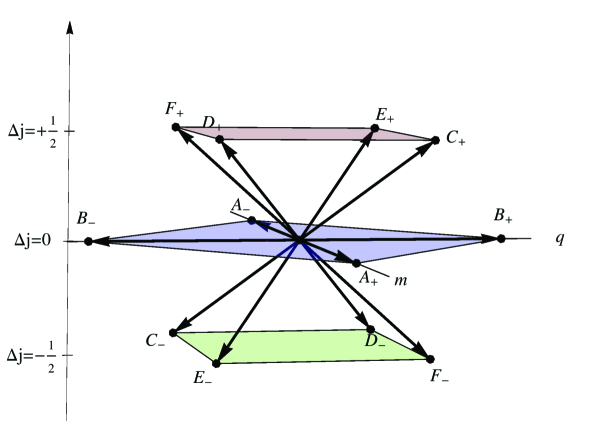
Figure 3: Action of the ladder operators on the Jacobi functions ${\cal J}_{j}^{(m,q)}(x)$ represented by the triplets $(j,m,q)$. The planes displayed correspond to the pairs $(m,q)$, the parameter $j$ (or $\Delta j$) is represented in the vertical axis.

All these differential operators act on the space $\{{\cal J}_{j}^{m,q}\}$ for $j,m,q$ integer and half-integer such that $j\geq|m|,|q|$. The explicit form of their action is:

$$\begin{array}[]{rcl}C_{+}\,{\cal J}_{j}^{m,q}(x)&=&\sqrt{(j+m+1)(j+q+1)}\;{\cal J}_{j+1/2}^{m+1/2,\;q+1/2}(x),\\[11.38092pt] C_{-}\,{\cal J}_{j}^{m,q}(x)&=&\sqrt{(j+m)(j+q)}\;{\cal J}_{j-1/2}^{m-1/2,\;q-1/2}(x),\\[11.38092pt] D_{+}\,{\cal J}_{j}^{m,q}(x)&=&\sqrt{(l+m+1)(l-q+1)}\;{\cal J}_{j+1/2}^{m+1/2,\;q-1/2}(x)\\ \\ D_{-}\,{\cal J}_{j}^{m,q}(x)&=&\sqrt{(j+m)(j-q)}\;{\cal J}_{j-1/2}^{m-1/2,\,q+1/2}(x,)\\[11.38092pt] E_{+}\,{\cal J}_{j}^{m,q}(x)&=&\sqrt{(j-m+1)\,(j+q+1)}\;{\cal J}_{j+1/2}^{m-1/2,\;q+1/2}(x),\\[11.38092pt] E_{-}\,{\cal J}_{j}^{m,q}(x)&=&\sqrt{(j-m)\,(j+q)}\;{\cal J}_{j-1/2}^{m+1/2,\;q-1/2}(x),\\[11.38092pt] F_{+}\,{\cal J}_{j}^{m,q}(x)&=&\sqrt{(j-m+1)\,(j-q+1)}\;\,{\cal J}_{j+1/2}^{m-1/2,\,q-1/2}(x),\\[11.38092pt] F_{-}\,{\cal J}_{j}^{m,q}(x)&=&\sqrt{(j-m)\,(j-q)}\;{\cal J}_{j-1/2}^{m+1/2,\;q+1/2}(x).\end{array}$$ (4.2)

From (4.2) (or (4.1) remembering the order in the operators) we have

$$C_{\pm}^{\dagger}=C_{\mp},\qquad D_{\pm}^{\dagger}=D_{\mp},\qquad E_{\pm}^{\dagger}=E_{\mp},\qquad F_{\pm}^{\dagger}=F_{\mp},$$

i.e. all these rising/lowering operators have the hermiticity properties required by the representation to be unitary. The operators (4.1) change all parameters by $\pm 1/2$. We define all together $X_{\pm}$ the ones that change $j$ in $j\pm 1/2$, that in Fig. 3 correspond to the planes $\Delta j=\pm 1/2$.

From the eqs. (4.1) it is easily stated that

$$\begin{array}[]{llr}D_{\pm}(X,D_{x},M,Q)&=&C_{\pm}(-X,-D_{x},M,-Q),\\[8.5359pt] E_{\pm}(X,D_{x},M,Q)&=&C_{\pm}(-X,-D_{x},-M,Q),\\[8.5359pt] F_{\pm}(X,D_{x},M,Q)&=&-C_{\pm}(X,D_{x},-M,-Q).\end{array}$$ (4.3)

Thus, because of the Weyl symmetry of the roots, we limit ourselves to discuss the operators $C_{\pm}$. Taking thus into account their action on the Jacobi functions we get

$$[C_{+},C_{-}]=-2C_{3},\qquad[C_{3},C_{\pm}]=\pm C_{\pm}$$ (4.4)

where

$$C_{3}:=J+\frac{1}{2}(M+Q)+\frac{1}{2}.$$ (4.5)

Hence $\{C_{\pm},C_{3}\}$ close a $su(1,1)$ algebra that is denoted $su_{C}(1,1)$.

As in the cases of the operators $A_{\pm}$ and $B_{\pm}$, we obtain the Jacobi differential equation up to a non vanishing factor from the Casimir ${\cal C}_{C}$ of $su_{C}(1,1)$, written in terms of (4.1) and (4.5),

$${\cal C}_{C}{\cal J}_{j}^{m,q}(x)\equiv\left[C_{3}^{2}-\frac{1}{2}\{C_{+},C_{-}\}\right]{\cal J}_{j}^{m,q}(x)=\frac{1}{4}\left[(m+q)^{2}-1\right]{\cal J}_{j}^{m,q}(x).$$ (4.6)

Indeed

$$\begin{array}[]{l}\displaystyle\left[{\cal C}_{C}-\frac{1}{4}(M+Q)^{2}+\frac{1}{4}\right]\;{\cal J}_{j}^{m,q}(x)\\[14.22636pt] \qquad\equiv\left[C_{3}^{2}-\frac{1}{2}\{C_{+},C_{-}\}-\frac{1}{4}\,(M+Q)^{2}+1/4\right]\,{\cal J}_{j}^{m,q}(x)=0\end{array}$$ (4.7)

allows us to recover the Jacobi eq. (3.4). Analogously the same result derives from eqs.

$$\begin{array}[]{l}\left[C_{+}\,C_{-}-(J+M)\,(J+Q)\right]\;{\cal J}_{j}^{m,q}(x)=0,\\[11.38092pt] \left[C_{-}\,C_{+}-(J+1+M)\,(J+1+Q)\right]\;{\cal J}_{j}^{m,q}(x)=0,\end{array}$$ (4.8)

obtained by the factorization method.

From (4.7) we see that since $(m+q)=0,\pm 1,\pm 2,\pm 3,\cdots$ the IR of su(1, 1) with ${\cal C}_{C}=(m+q)^{2}/4-1/4=-1/4,0,3/4,2,15/4,\cdots$ are obtained. Hence, the set of AJF supports many infinite dimensional UIR, of $SU(1,1)$ of the discrete series for $SU_{C}(1,1)$ [24].

Similar results can be found for the other ladder operators $D\pm,E\pm,F\pm$ with the substitutions (4.3) in all eqs. (4.4-4.8).

5 The complete symmetry group of $\{{\cal J}_{j}^{m,q}(x)\}$: $SU(2,2)$

If one represents the action of the twelve operators $A_{\pm},B_{\pm},C_{\pm},D_{\pm},E_{\pm},F_{\pm}$, that we have defined in previous sections, we obtain Fig. 3. To obtain the root system of the simple Lie algebra $A_{3}\equiv D_{3}$ we have only simply to add three points in the origin corresponding to the elements $J,M$ and $Q$ of the Cartan subalgebra.

The Lie commutators of the generators $A_{\pm},B_{\pm},C_{\pm},D_{\pm},E_{\pm},F_{\pm},J,M,Q$ are

$$\begin{array}[]{llll}[J,A_{\pm}]=0,&[J,M]=0,&[J,B_{\pm}]=0,&[J,Q]=0,\\[11.38092pt] [J,C_{\pm}]=\pm\frac{1}{2}\,C_{\pm},&[J,D_{\pm}]=\pm\frac{1}{2}\,D_{\pm},&[J,E_{\pm}]=\pm\frac{1}{2}\,E_{\pm},&[J,F_{\pm}]=\pm\frac{1}{2}\,F_{\pm},\\[11.38092pt] [M,B_{\pm}]=0,&[M,Q]=0,&&\\[11.38092pt] [M,C_{\pm}]=\pm\frac{1}{2}\,C_{\pm},&[M,D_{\pm}]=\pm\frac{1}{2}\,D_{\pm},&[M,E_{\pm}]=\mp\frac{1}{2}\,E_{\pm},&[M,F_{\pm}]=\mp\frac{1}{2}\,F_{\pm},\\[11.38092pt] [Q,A_{\pm}]=0,&&&\\[11.38092pt] [Q,C_{\pm}]=\pm\frac{1}{2}\,C_{\pm},&[Q,D_{\pm}]=\mp\frac{1}{2}\,D_{\pm},&[Q,E_{\pm}]=\pm\frac{1}{2}\,E_{\pm},&[Q,F_{\pm}]=\mp\frac{1}{2}\,F_{\pm},\\[11.38092pt] [A_{+},A_{-}]=2A_{3},&[A_{3},A_{\pm}]=\pm A_{\pm},&(A_{3}=M),&\\[11.38092pt] [B_{+},B_{-}]=2B_{3},&[B_{3},B_{\pm}]=\pm B_{\pm},&(B_{3}=Q),&\\[11.38092pt] [C_{+},C_{-}]=-2C_{3},&[C_{3},C_{\pm}]=\pm C_{\pm},&(C_{3}=J+\frac{1}{2}(M+Q)+\frac{1}{2}),&\\[11.38092pt] [D_{+},D_{-}]=-2D_{3},&[D_{3},D_{\pm}]=\pm D_{\pm},&(D_{3}=J+\frac{1}{2}(M-Q)+\frac{1}{2}),&\\[11.38092pt] [E_{+},E_{-}]=-2E_{3},&[E_{3},E_{\pm}]=\pm E_{\pm},&(E_{3}=J+\frac{1}{2}(-M+Q)+\frac{1}{2}),&\\[11.38092pt] [F_{+},F_{-}]=-2F_{3},&[F_{3},F_{\pm}]=\pm F_{\pm},&(F_{3}=J-\frac{1}{2}(M+Q)+\frac{1}{2}),&\\[11.38092pt] [A_{\pm},B_{\pm}]=0,&[A_{\pm},B_{\mp}]=0,&&\\[11.38092pt] [A_{\pm},C_{\pm}]=0,&[A_{\pm},C_{\mp}]=\pm E_{\mp},&[A_{\pm},D_{\pm}]=0,&[A_{\pm},D_{\mp}]=\mp F_{\mp},\\[11.38092pt] [A_{\pm},E_{\pm}]=\pm C_{\pm},&[A_{\pm},E_{\mp}]=0,&[A_{\pm},F_{\pm}]=D_{\pm},&[A_{\pm},F_{\mp}]=0,\\[11.38092pt] [B_{\pm},C_{\pm}]=0,&[B_{\pm},C_{\mp}]=\mp D_{\mp},&[B_{\pm},D_{\pm}]=\pm C_{\pm},&[B_{\pm},D_{\mp}]=0,\\[11.38092pt] [B_{\pm},E_{\pm}]=0,&[B_{\pm},E_{\mp}]=\mp F_{\mp},&[B_{\pm},F_{\pm}]=\pm E_{\pm},&[B_{\pm},F_{\mp}]=0,\\[11.38092pt] [C_{\pm},D_{\pm}]=0,&[C_{\pm},D_{\mp}]=\mp B_{\pm},&[C_{\pm},E_{\pm}]=0,&[C_{\pm},E_{\mp}]=\mp A_{\pm},\\[11.38092pt] [C_{\pm},F_{\pm}]=0,&[C_{\pm},F_{\mp}]=0,&&\end{array}$$

$$\begin{array}[]{llll}[D_{\pm},E_{\pm}]=0,&[D_{\pm},E_{\mp}]=0,&[D_{\pm},F_{\pm}]=0,&[D_{\pm},F_{\mp}]=\mp A_{\pm},\\[11.38092pt] [E_{\pm},F_{\pm}]=0,&[E_{\pm},F_{\mp}]=\mp B_{\pm}.&&\end{array}$$

The quadratic Casimir of $su(2,2)$ has the form

$$\begin{array}[]{ll}{\cal C}_{su(2,2)}&=\displaystyle\frac{1}{2}\left(\{A_{+},A_{-}\}+\{B_{+},~{}B_{-}\}-\{C_{+},C_{-}\}-\{D_{+},D_{-}\}-\{E_{+},E_{-}\}-\{F_{+},F_{-}\}\right)\\[8.5359pt] &\qquad\qquad\displaystyle+\,\frac{1}{2}\,\left(A_{3}^{2}+B_{3}^{2}+C_{3}^{2}+D_{3}^{2}+E_{3}^{2}+F_{3}^{2}\right)\\[11.38092pt] &=\displaystyle\frac{1}{2}\left(\{A_{+},A_{-}\}+\{B_{+},~{}B_{-}\}-\{C_{+},C_{-}\}-\{D_{+},D_{-}\}-\{E_{+},E_{-}\}-\{F_{+},F_{-}\}\right)\\[8.5359pt] &\qquad\qquad\displaystyle+\,2J(J+1)+M^{2}+Q^{2}+\frac{1}{2}\\[11.38092pt] &\displaystyle\equiv-\frac{3}{2}.\end{array}$$

From it and taking into account the differential realization of the operators involved, (3.1), (3.6) and (4.1), we recover again the Jacobi equation (3.4).

Hence, the AJF support a UIR of the group $SU(2,2)$ with the value -3/2 of ${\cal C}_{su(2,2)}$ (see Fig. 4). Also, as we have seen along the previous sections, the Jacobi equations is recovered form the Casimir of any subalgebra of ${su(2,2)}$ as well as from any diagonal product of ladder operators.

In this UIR of $SU(2,2)$ the integer and half-integer values of $(j,m,q)$ are putted all together. The symmetries where integer and half-integer values belong to different UIR will be discussed in next Section.

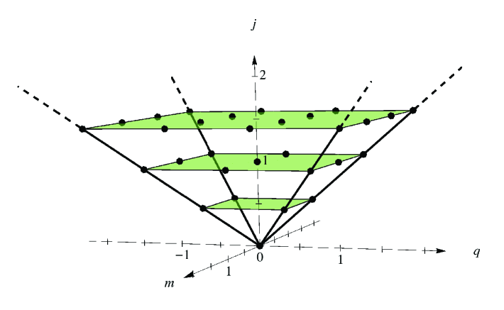
Figure 4: IR of $su(2,2)$ supported by the AJF ${\cal J}_{l}^{m,q}(x)$ represented by the black points. The horizontal planes correspond to IR of $su_{A}(2)\oplus su_{B}(2)$.

6 Symmetries inside integers/half-integers labels

In the preceding sections we have obtained a set of symmetries on the AJF ${\cal J}_{j}^{m,q}(x)$ where the operators $A_{\pm}$ ($B_{\pm}$) change only the label $m$ ($q$) of $\pm 1$ leaving invariant the remaining two labels and the other operators $X_{\pm}$ of the algebra change all the $(j,m,q)$ by a half-integer quantity. Integer and half-integer values of $(j,m,q)$ are indeed related to a unique UIR of $SU(2,2)$.

Now, composing the action ot pairs of operators $X_{\pm}$ , we can construct two operators that change $(j,m,q)$ to $(j\pm 1,m,q)$. Indeed $F_{\pm}C_{\pm}$ (equivalently, $C_{\pm}F_{\pm}$, $D_{\pm}E_{\pm}$ or $E_{\pm}D_{\pm}$) are such operators. Moreover they, in general second order differential operators, reduce –because of the Jacobi equation (3.4)– to a first order differential operators when applied to the ${\cal J}_{j}^{m,q}$.

As discussed before  the ${\cal J}_{j}^{m,q}$ have $j\geq|m|$ and $j\geq|q|$, but now we have to consider separately specific values of $m$ and $q$.

To begin with let us start with states such that $j\geq|m|>|q|$ . From (4.1) and (3.4) we get that the two conjugate hermitian operators

$$K_{+}:=F_{+}C_{+}\frac{1}{\sqrt{(J+1)^{2}-Q^{2}}},\qquad K_{-}:=F_{-}C_{-}\frac{1}{\sqrt{J^{2}-Q^{2}}}$$ (6.1)

can be written on the AJF as

$$K_{+} := \left(-(1-X^{2})\;D_{x}+X\;(J+1)+\frac{MQ}{J+1}\;\right)\frac{J+1}{\sqrt{(J+1)^{2}-Q^{2}}}$$ (6.2)

$$K_{-} := \left((1-X^{2})\;D_{x}+X\;J+\frac{MQ}{J}\right)\frac{J}{\sqrt{J^{2}-Q^{2}}}\;$$ (6.3)

always well defined because $j>|q|$ on these AJF. By inspection, their action does not depend from the value of $q$:

$$\begin{array}[]{lll}K_{+}\;{\cal J}_{j}^{m,q}(x)&=&\,\sqrt{(j+1)^{2}-m^{2}}\;{\cal J}_{j+1}^{m,q}(x),\\[8.5359pt] \displaystyle K_{-}\;{\cal J}_{j}^{m,q}(x)&=&\,\sqrt{j^{2}-m^{2}}\;{\cal J}_{j-1}^{m,q}(x),\end{array}$$ (6.4)

and $K_{\pm}$ together with $K_{3}:=J+1/2$ close a $su(1,1)$ Lie algebra

$$[K_{+},K_{-}]=-2K_{3},\qquad[K_{3},K_{\pm}]=\pm K_{\pm}$$

such that the ${\cal J}_{j}^{m,q}$ with $m$ and $q$ fix and  $j\geq|m|>|q|$  are a basis of the UIR of $su(1,1)$ with Casimir

$${\cal C}=m^{2}-1/4.$$

For the states where  $|m|<|q|$  the procedure is analogous: we have only to interchange $M\Leftrightarrow Q$ in $K_{\pm}$.

The problem is more complex when $|m|=|q|$ as the action of $K_{-}$ is not well defined in eq.(6.3) for $j=|m|=|q|$. To extend its definition to this case we have to consider not the eigenvalues of $M$ and $Q$ but their limit  i.e.

$$K_{-}:=\lim_{\epsilon\to 0}\left[\left((1-X^{2})\,D_{x}+X\,J+\frac{(M+\epsilon)(Q+\epsilon)}{J}\right)\frac{J}{\sqrt{J^{2}-(Q+\epsilon)^{2}}}\;\right].$$

In this way the action of $K_{-}$ does not change for $j>|m|=|q|$ while for $j=|m|=|q|$, results from the product of a first factor that goes like $\epsilon$ an a second one that goes like $\epsilon^{-1/2}$ and it is thus zero.

In conclusion, all  ${\cal J}_{j}^{m,q}$  close, for fixed $m$ and $q$, a UIR of $SU(1,1)$. If $|m|\geq|q|$ we have eqs. (6.4) with $j=|m|,|m|+1,|m|+2\dots$ and Casimir invariant ${\cal C}=m^{2}-1/4$ while, for $|m|<|q|$, we have to exchange everywhere $q$ and $m$.

Note that, unlike the UIR of $SU(2,2)$, each representation of $SU(1,1)$ contains only states with integer or half-integer values of its labels. This is particularly relevant for the $d^{j}_{q\,m}$ as usual symmetries in physics do not mix integer and half-integer spins  i.e. bosons and fermions.

This $SU(1,1)$ cannot in general be extended to larger groups as its operators cannot be combined with other operators to construct a bigger algebra, but there are few exceptions. Indeed when $q=0$, i.e. on the ${\cal J}_{j}^{m,0}$ with $j,m\in{\mathbb{Z}}$ and $j\geq|m|$, we can define not only the $\{K_{\pm},K_{3}\}$ but also the $\{A_{\pm},A_{3}\}$ and thus the whole algebra $so(3,2)$ described in [12]. The $\{{\cal J}_{j}^{m,0}\}$ are indeed related to the Associate Legendre Polynomials $P_{n+{\alpha}}^{{\alpha}}$ and thus a basis of a UIR of $SO(3,2)$. By inspection $K_{\pm}$ are exactly the ones reported in fomulas (2.13-14) of [12] and $A_{\pm}$ are the $J_{\pm}$ of formulas (2.11-12) of the same paper. Because of the symmetry $m\Leftrightarrow q$ we have a $SO(3,2)$ also for $m=0$ i.e. on the $\,\{{\cal J}_{j}^{0,q}\}\,$.

Also ”fermions” states $\{{\cal J}_{j}^{m,\pm 1/2}\}$ and $\{{\cal J}_{j}^{\pm 1/2,q}\}\,$ are related to the same algebra $so(3,2)$ but, of course, to a representation of its covering group $Spin(3,2)$ [25].

7 $L^{2}$–functions spaces and ${\cal J}_{j}^{m,q}(x)$

As already discussed in details in [11] and [12], special functions together with their Lie group properties play a role in $L^{2}$–functions and Hilbert spaces.

Formulas (2.7) and (2.8) where $m$ and $q$ are fixed allow to introduce $j$ and $x$ as conjugate variables on the same Hilbert space. Let us thus begin discussing the case of section 6, where $m$ and $q$ are fixed parameters characterizing the UIR of $su(1,1)$ and its support Hilbert space.

Operators (6.1) written as (6.4) on the $\{{\cal J}_{j}^{m,q}(x)\}$ allow to define, in abstract form, for fixed $m$ and $q$, the action on a Hilbert space constructed in the space of eigenvectors  $\{|j,(m,q)\rangle\}$  of the operators $J$  as

$$\begin{array}[]{lll}K_{+}\;|j,(m,q)\rangle&=&\,\sqrt{(j+1)^{2}-m^{2}}\;|j+1,(m,q)\rangle,\\[8.5359pt] \displaystyle K_{-}\;|j,(m,q)\rangle&=&\,\sqrt{j^{2}-m^{2}}\;|j-1,(m,q)\rangle.\end{array}$$ (7.1)

and $\{|j,(m,q)\rangle\}$ is a basis of the Hilbert space  i.e.

$$\langle j,(m,q)|j^{\prime},(m,q)\rangle=\delta_{j\,j^{\prime}}\qquad\sum_{j={\it sup}(|m|,|q|)}^{\infty}|j,(m,q)\rangle\;\langle j,(m,q)|={\cal I}.$$ (7.2)

This allows to define

$$|x,(m,q)\rangle:=\;\sum_{j={\it sup}(|m|,|q|)}^{\infty}|j,(m,q)\rangle\,\sqrt{j+1/2}\;\,{\cal J}_{j}^{m,q}(x)$$ (7.3)

where the vectors $\{|x,(m,q)\rangle\}$ are a basis of the configuration space ${\mathbb{E}}=(-1,1)\subset{\mathbb{R}}$ i.e.

$$\langle x,(m,q)|x^{\prime},(m,q)\rangle=\delta(x-x^{\prime})\quad\qquad\int_{-1}^{+1}|x,(m,q)\rangle\,dx\,\langle x,(m,q)|\;=\,{\cal I}\;.$$

This implies that the $\{{\cal J}_{j}^{m,q}(x)\}$ are the transition matrices between the two bases:

$${\cal J}_{j}^{m,q}(x)\,=\,\frac{1}{\sqrt{j+1/2}}\;\langle x,(m,q)|j,(m,q)\rangle\,=\,\frac{1}{\sqrt{j+1/2}}\;\langle j,(m,q)|x,(m,q)\rangle\;.$$

and

$$|j,(m,q)\rangle=\int_{-1}^{+1}|x,(m,q)\rangle\,\sqrt{j+1/2}\;\,{\cal J}_{j}^{m,q}(x)\,dx\;.$$ (7.4)

As $m$ and $q$ are invariant of the representation, this situation is similar to the Lagrange functions discussed in [11], where only two conjugate variables $j$ and $x$ (one discrete and one continuous) are present. The difference is that in [11] a basis was associated to each element $\mathfrak{g}$ of the group $SU(1,1)$, while here we have a basis for each element of the triple $(m,q,\mathfrak{g})$.

The case of two discrete variables, related to the group $SO(3,2)$, has been discussed in [12] and it will be not reconsidered here. On the contrary we consider the new case of three variables case, related to $SU(2,2)$ where both $m$ and $q$ are modified by the algebra.

The Hilbert space is now ${\mathbb{E}}\times{\mathbb{Z}}\times{\mathbb{Z}}/2$ , where ${\mathbb{E}}$ is again $(-1,1)\subset{\mathbb{R}}$, ${\mathbb{Z}}/2:=\{0,\pm 1/2,\pm 1,\pm 3/2,\pm 2,\cdots\}$ is related to $m$ and ${\mathbb{Z}}$ to $m-q$, as $m$ and $q$ are together integer or half-integer. The space ${\mathbb{E}}\times{\mathbb{Z}}\times{\mathbb{Z}}/2$, with basis $\{|x,m,q\rangle\}$, is the direct sum of the Hilbert spaces ${\mathbb{E}}_{m,q}$ with $m$ and $q$ fixed,

$${\mathbb{E}}\times{\mathbb{Z}}\times{\mathbb{Z}}/2=\bigcup_{m-q\in{\mathbb{Z}}}\;\bigcup_{q\in{\mathbb{Z}}/2}\;{\mathbb{E}}_{m,q}.$$

Orthonormality and completeness are now,

$$\langle x,m,q|x^{\prime},m^{\prime},q^{\prime}\rangle\;=\;\delta(x-x^{\prime})\,\delta_{m\,m^{\prime}}\,\,\delta_{q\,q^{\prime}},\qquad\sum_{m,q}\,\int_{-1}^{+1}|x,m,q\rangle\,dx\,\langle x,m,q|\;=\;{\cal I}.$$

Analogously to (7.4) we can now define inside the Hilbert space a new basis $\{|j,m,q\rangle\}$ with $m,q\in{\mathbb{Z}}/2,\;j\geq|m|,\;j\geq|q|,\;j-m\in{\mathbb{N}},\;j-q\in{\mathbb{N}}$ by

$$|j,m,q\rangle:=\int_{-1}^{+1}|x,m,q\rangle\,\sqrt{j+1/2}\;\,{\cal J}_{j}^{m,q}(x)\,dx\;.$$

so that

$$\langle j,m,q^{\prime}|j^{\prime},m^{\prime},q^{\prime}\rangle\;=\;\delta_{j\,j^{\prime}}\,\delta_{m\,m^{\prime}}\,\delta_{q,\,q^{\prime}},\qquad\sum_{j,m,q}|j,m,q\rangle\;\langle j,m,q|\;=\;{\cal I}.$$

The $\{{\cal J}_{j}^{m,q}(x)\}$ plays the role of transition matrices:

$${\cal J}_{j}^{m,q}(x)=\frac{1}{\sqrt{j+1/2}}\;\langle x,m,q|j,m,q\rangle=\frac{1}{\sqrt{j+1/2}}\;\langle j,m,q|x,m,q\rangle\;.$$

Like in Ref. [11, 12] the role of the algebraic Jacobi functions $\{{\cal J}_{j}^{m,q}(x)\}$ as transition matrices reflects the fact that the generators can be seen as differential operators in ${\mathbb{E}}\times{\mathbb{Z}}\times{\mathbb{Z}}/2$, or algebraic operators in the spaces of labels ${\mathbb{N}}/2\times{\mathbb{N}}\times{\mathbb{N}}$, where ${\mathbb{N}}/2$ is related to $j$ and the two ${\mathbb{N}}$ to $j-m$ and $j-q$. This allows to make explicit the Lie algebra structure in contrast with Ref. [7, 8, 9].

An arbitrary vector $|f\rangle\,\in L^{2}({\mathbb{E}},{\mathbb{Z}},{\mathbb{Z}}/2)$ can be alternatively expressed as

$$|f\rangle\;=\;\sum_{m,q=-\infty}^{\infty}\int_{-1}^{+1}dx\;|x,m,q\rangle\,f^{m,q}(x)\;=\sum_{m,q=-\infty}^{+\infty}\;\;\;\sum_{j=sup(|m|,|q|)}^{\infty}|j,m,q\rangle\;f^{m,q}_{j}$$

where

$$\begin{array}[]{lllll}f^{m,q}(x)&:=&\langle x,m,q|f\rangle&=&\displaystyle\sum_{j=sup(|m|,|q|)}^{\infty}\sqrt{j+1/2}\;{\cal J}_{j}^{m,q}(x)\,f_{j}^{m,q},\\[14.22636pt] f_{j}^{m,q}&:=&\langle j,m,q|f\rangle&=&\displaystyle\int_{-1}^{+1}dx\;\sqrt{j+1/2}\;{\cal J}_{j}^{m,q}(x)\,f^{m,q}(x)\end{array}$$

and all the $L^{2}$–functions defined on $({\mathbb{E}},{\mathbb{Z}},{\mathbb{Z}}/2)$ can be written as

$$\sum_{m,q=-\infty}^{\infty}\;\sum_{j=sup(|m|,|q|)}^{\infty}\;\sqrt{j+1/2}\;{\cal J}_{j}^{m,q}(x)\;f_{j}^{m,q}.$$ (7.5)

As the  $\{{\cal J}_{j}^{m,q}\}$  are a basis of a UIR of $SU(2,2)$ and  (see eq.(7.5)), at the same time, a basis of the $L^{2}$–functions defined on $({\mathbb{E}},{\mathbb{Z}},{\mathbb{Z}}/2)$ the $L^{2}({\mathbb{E}},{\mathbb{Z}},{\mathbb{Z}}/2)$ belong to the same UIR of $SU(2,2)$. This implies that every change of basis in the $L^{2}({\mathbb{E}},{\mathbb{Z}},{\mathbb{Z}}/2)$ is related to an element $\mathfrak{g}$ of the group $SU(2,2)$ and that every operators that acts on the $L^{2}({\mathbb{E}},{\mathbb{Z}},{\mathbb{Z}}/2)$ can be written inside the Universal Enveloping Algebra of $su(2,2)$.

8 Conclusions

The algebraic Jacobi functions are a particular case of the algebraic special functions recently introduced by us [11, 12] whose relevance seems to be related to the following points:

1. The role of intertwining between second order differential equations and Lie algebras played by the algebraic special functions.

2. Peculiar properties of the algebraic special functions, that perhaps could be assumed as their definition, look to be that – taking into account the fundamental second order differential equation – all diagonal elements of the UEA can be found to be related to it and that all non-diagonal elements can be written as first order differential operators.

3. The fact that ASF (here AJF) are at the same time an irreducible representation of a Lie algebra (here $su(2,2)$) and a basis of $L^{2}$–functions (here the ones defined on ${\mathbb{E}}\times{\mathbb{Z}}\times{\mathbb{Z}}/2)$ allows to establish a homorphism between the UEA of the Lie algebra and the vector space of the operators defined on the $L^{2}$–functions. In this way the framework of Quantum Mechanics is reproduced with $L^{2}({\mathbb{E}},{\mathbb{Z}},{\mathbb{Z}}/2)$ Hilbert space and $su(2,2)$-UEA as space of operators acting on it.

4. As the ASF are a basis of a unitary irreducible representation of the corresponding Lie group also, all sets obtained from ASF applying an element $\mathfrak{g}$ of the Lie group are bases in the space of the $L^{2}$–functions. Moreover in the $SU(1,1)$ cases presented in Sect. 6 each basis depends not only on the group element $\mathfrak{g}$ but also on the pair $(m,q)$.

5. Although the UIR of $SU(2,2)$ put together integer and half-integer values of the labels $(j,m,q)$, the analysis of Sect. 6 separates boson and fermions systems as usual in physical applications. In this case $L^{2}({\mathbb{E}})$ is the Hilbert space and $su(1,1)$-UEA is the space of operators acting on it.

6. The algebraic Jacobi functions have the same symmetry of the elements of the $d_{j}$-matrices. This enhances the interest of the algebraic special functions in physical applications since the Wigner matrices play an important role in the description of Quantum Mechanics.

References

- [1] M. Berry, Phys. Today 54 (2001) 11.
- [2] G.E. Andrews, R. Askey, R. Roy, Special Functions, Cambrige Univ. Press, Cambridge, 1999.
- [3] G. Heckman, H. Schlichtkrull, Harmonic Analysis and Special Functions on Symmetric Spaces, Academic Press, New York, 1994.
- [4] R. Koekoek, P.A. Lesky, R.F. Swarttouw, Hypergeometric Orthogonal Polynomials and Their -Analogues, Springer, Berlin, 2010 (and references therein).
- [5] E.P. Wigner, The application of group theory to the special functions of mathematical physics, in: Princeton Lectures, 1955.
- [6] J.D. Talman, Special functions: a group theoretic approach, Benjamin, New York, 1968.
- [7] W. Miller, Lie Theory and Special Functions, Academic Press, New York, 1968.
- [8] N. Ja. Vilenkin, Special Functions and the Theory of Group Representations, Amer. Math. Soc., Providence, 1968.
- [9] N. Ja. Vilenkin, A.U. Klimyk, Representation of Lie Groups and Special Functions vols. 1, 2 and 3, Kluwer, Dordrecht, 1991, 1993 and 1992 (and references therein).
- [10] N. Ja. Vilenkin, A.U. Klimyk, Representation of Lie Groups and Special Functions: Recent Advances, Kluwer, Dordrecht, 1995.
- [11] E. Celeghini, M.A. del Olmo, Ann. of Phys. 335 (2013) 78.
- [12] E. Celeghini, M.A. del Olmo, Ann. of Phys. 333 (2013) 90.
- [13] C. Truesdell, Annals in Math. Studies 18, Princeton Univ. Press, Princeton, 1948.
- [14] S. Cambianis, Proc. of the Am. Math. Soc. 29 (1971) 284.
- [15] E. Celeghini, M.A. del Olmo, M. A. Velasco, Jacobi Polynomials and , arXiv:1307.7380.
- [16] F.W.J. Olver, D.W. Lozier, R.F. Boisvert, C.W. Clark, NIST Handbook of Mathematical Functions, Cambridge Univ. Press, New York, 2010.
- [17] Y.L. Luke, The Special Functions and Their Approximations Vol.1, Academic Press, San Diego, 1969 (pp. 275–276).
- [18] M. Abramowitz, I. Stegun, Handbook of Mathematical Functions with Formulas, Graphs, and Mathematical Tables, Dover, San Diego, 1972.
- [19] L.C. Biedenharn and J.D. Louck, Angular Momentum in Quantum Mechanics, Addison-Wesley, Reading, 1981
- [20] E. Wigner, Zeitschrift für Physik 43 (1927) 624.
- [21] Wu-Ki Tung, Group Theory in Physics, World Scientific, Singapore (1985).
- [22] E. Schrödinger, Proc. Roy. Irish Acad. A46, 183 (1940); A47 (1941) 53.
- [23] L. Infeld, T.E. Hull, Rev. Mod. Phys. 23 (1951) 21.
- [24] V. Bargmann, Ann. of Math. 48 (1947) 368.
- [25] H.B. Lawson, M.L. Michelsohn, Spin Geometry, Princeton Univ. Press, Princeton, 1989.