Exporting superconductivity across the gap: Proximity effect for semiconductor valence-band states due to contact with a simple-metal superconductor

Abstract

The proximity effect refers to the phenomenon whereby superconducting properties are induced in a normal conductor that is in contact with an intrinsically superconducting material. In particular, the combination of nano-structured semiconductors with bulk superconductors is of interest because these systems can host unconventional electronic excitations such as Majorana fermions when the semiconductor’s charge carriers are subject to a large spin-orbit coupling. The latter requirement generally favors the use of hole-doped semiconductors. On the other hand, basic symmetry considerations imply that states from typical simple-metal superconductors will predominantly couple to a semiconductor’s conduction-band states and, therefore, in the first instance generate a proximity effect for band electrons rather than holes. In this article, we show how the superconducting correlations in the conduction band are transferred also to hole states in the valence band by virtue of inter-band coupling. A general theory of the superconducting proximity effect for bulk and low-dimensional hole systems is presented. The interplay of inter-band coupling and quantum confinement is found to result in unusual wave-vector dependencies of the induced superconducting gap parameters. One particularly appealing consequence is the density tunability of the proximity effect in hole quantum wells and nanowires, which creates new possibilities for manipulating the transition to nontrivial topological phases in these systems.

I Introduction & Motivation

Superconductor-semiconductor heterostructures have been the subject of intense study Hekking et al. (1994); Beenakker ; van Wees and Takayanagi ; Lambert and Raimondi (1998); Schäpers (2001); Takayanagi et al. (2008) because they offer intriguing possibilities to observe effects of quantum phase coherence in electronic transport Akkermans et al. (1995); Sohn et al. (1997); Beenakker (1997). The contact to a superconducting material induces pair correlations of charge carriers in the semiconductor and, especially in low-dimensional or nanostructured systems, results in a gapped spectrum of electronic excitations de Gennes (1964); Volkov et al. (1995); Fagas et al. (2005); Kopnin and Melnikov (2011). Recent work has focused on the interplay of proximity-induced superconductivity and strong spin-orbit coupling in nanowires Lutchyn et al. (2010); Oreg et al. (2010); Sau et al. (2010); Alicea (2010); Klinovaja et al. (2012); Zyuzin et al. (2013), which can give rise to the presence of unconventional quasiparticle excitations Alicea (2012); Leijnse and Flensberg (2012); Beenakker (2013); Stanescu and Tewari (2013). As the charge carriers from the valence band of typical semiconductors ("holes") are generically subject to particularly strong spin-orbit-coupling effects Winkler (2003); Kloeffel et al. (2011), it has been suggested Mao et al. (2011, 2012) that the use of hole-doped nanowires is a good strategy for experimental realization and detailed study of exotic quasiparticles. These developments have created a need for a fundamental, and experimentally relevant, theoretical description of the proximity effect for holes, which we are providing in this work.

We consider heterostructures consisting of a bulk superconductor in contact with semiconductors of varying dimensionality. The superconducting material is assumed to be a simple metal, hence its unfilled band has s-like character and couples only to the semiconductor’s conduction-band states because these have compatible symmetry properties. (States from a typical semiconductor’s valence band have p-like symmetry Yu and Cardona (2010).) The resulting proximity effect can thus induce a gap only in the dispersion of charge carriers from the conduction band, leaving the valence band initially unaffected. However, as we show in greater detail below, the proximity-induced change in the electronic properties of the conduction band affects also valence-band states via the ubiquitous interband coupling Kane (1957); Winkler (2003); Yu and Cardona (2010) that is present at finite wave vector ${\bm{\mathrm{k}}}$. Previous work Futterer et al. (2011) has investigated how Andreev reflection of holes is enabled, and its characteristics changed from that occurring at ordinary superconductor–normal-metal interfaces Andreev (1964); de Gennes and Saint-James (1963), by interband coupling. Here we generalize this concept to develop a fundamental study of how superconducting correlations translate from the conduction band into the valence band. In particular, the method of Löwdin partitioning Winkler (2003) is employed to derive the effective Bogoliubov-de Gennes (BdG) Hamiltonian de Gennes (1989) that governs the proximity effect for holes, thus providing a starting point for further detailed studies of topological phases in hole-doped semiconductor nanostructures Mao et al. (2011, 2012).

The remainder of this article is organized as follows. Basics of the mathematical formalism are presented in Sec. II, together with the derivation of the effective Hamiltonian describing superconductivity of holes in semiconductors induced by a completely general interband coupling from the proximity effect in the conduction band. This result is then specialized in Sec. III to the case of the Kane-model description Kane (1957); Winkler (2003); Yu and Cardona (2010) of typical semiconductors. A comprehensive study of resulting changes to the electronic valence-band structure in bulk systems and various types of nanostructures is presented in Sec. IV. We provide a summary and conclusions of our work in Sec. V. Some mathematical details are given in the Appendix.

II Basic theory and general results

In order to derive the induced superconducting pair potential for the valence-band holes, we consider as a starting point the multi-band BdG Hamiltonian for a superconductor-semiconductor hybrid structure Futterer et al. (2011),

$${\mathcal{H}}_{\text{BdG}}=\left(\begin{array}[]{cccc}\mathsf{H}_{\text{c}}-\mu&\mathsf{H}_{\text{c-v}}&\Delta\,\openone_{2\times 2}&0_{2\times 4}\\ \mathsf{H}_{\text{c-v}}^{\dagger}&\mathsf{H}_{\text{v}}-\mu&0_{4\times 2}&0_{4\times 4}\\ \Delta^{\ast}\,\openone_{2\times 2}&0_{2\times 4}&\mu-\mathsf{H}_{\text{c}}&-\mathsf{H}_{\text{c-v}}\\ 0_{4\times 2}&0_{4\times 4}&-\mathsf{H}_{\text{c-v}}^{\dagger}&\mu-\mathsf{H}_{\text{v}}\end{array}\right)\,\,,$$ (1)

where $\mathsf{H}_{\text{c(v)}}$ is the effective-mass Hamiltonian of the conduction (valence) band, $\mathsf{H}_{\text{c-v}}$ describes the coupling between conduction and valence-band states, and $\Delta$ is the pair potential induced for conduction-band states only via contact to a simple-metal superconducting material. The matrix $\openone_{m\times m}$ is the identity matrix of dimension $m\times m$, and $0_{m\times n}$ is the zero matrix of dimension $m\times n$. The dimensionality for sub-blocks of ${\mathcal{H}}_{\text{BdG}}$ given in Eq. (1) is determined by the fact that charge carriers from the conduction (valence) band carry a spin-1/2 (spin-3/2) degree of freedom Yu and Cardona (2010). We adopt the representation where eigenstates for spin projections on the $z$ axis comprise the basis and use the order $|{\mathrm{c},+1/2}\rangle$, $|{\mathrm{c},-1/2}\rangle$ ($|{\mathrm{v},+3/2}\rangle$, $|{\mathrm{v},1/2}\rangle$, $|{\mathrm{v},-1/2}\rangle$, $|{\mathrm{v},-3/2}\rangle$) for spinor amplitudes of conduction-band (valence-band) states. The explicit form of the conduction and valence-band Hamiltonians depends on the particular model under consideration but, for typical semiconductor materials, the inter-band coupling is quite generally of the form Yu and Cardona (2010)

$$\mathsf{H}_{\text{c-v}}=\begin{pmatrix}-\frac{1}{\sqrt{2}}Pk_{+}&\sqrt{\frac{2}{3}}Pk_{z}&\frac{1}{\sqrt{6}}Pk_{-}&0\\ 0&-\frac{1}{\sqrt{6}}Pk_{+}&\sqrt{\frac{2}{3}}Pk_{z}&\frac{1}{\sqrt{2}}Pk_{-}\end{pmatrix}\,.$$ (2)

Here $P$ is the materials-dependent Kane-model Kane (1957) matrix element, and $k_{\pm}\equiv k_{x}\pm i\,k_{y}$ in terms of Cartesian coordinates of the band-electron wave vector ${\bm{\mathrm{k}}}$.

We can treat the inter-band coupling in lowest-order perturbation theory without needing to consider its explicit form, and thus derive a general effective Hamiltonian for the valence bands, by employing the Löwdin-partitioning method Winkler (2003). For completeness, and to motivate further approximations, we briefly sketch details of the calculation here. The BdG Hamiltonian [Eq. (1)] is split into a part $\mathcal{H}_{0}$ that describes the individual conduction and valence bands, and a part $\mathcal{H}_{1}$ that embodies the mixing between conduction and valence bands. We then have ${\mathcal{H}}_{\text{BdG}}=\mathcal{H}_{0}+\mathcal{H}_{1}$, with

$$\mathcal{H}_{1}=\left(\begin{array}[]{cccc}0_{2\times 2}&\mathsf{H}_{\text{c-v}}&0_{2\times 2}&0_{2\times 4}\\ \mathsf{H}_{\text{c-v}}^{\dagger}&0_{4\times 4}&0_{4\times 2}&0_{4\times 4}\\ 0_{2\times 2}&0_{2\times 4}&0_{2\times 2}&-\mathsf{H}_{\text{c-v}}\\ 0_{4\times 2}&0_{4\times 4}&-\mathsf{H}_{\text{c-v}}^{\dagger}&0_{4\times 4}\end{array}\right)\,\,.$$ (7)

The effective Hamiltonian for valence-band states that accounts for the presence of inter-band coupling can be found by performing a unitary transformation to eliminate the perturbation $\mathcal{H}_{1}$;

$$\tilde{{\mathcal{H}}}_{\text{BdG}}=\mathrm{e}^{-S}\leavevmode\nobreak\ {\mathcal{H}}_{\text{BdG}}\leavevmode\nobreak\ \mathrm{e}^{S}$$

$$\approx\mathcal{H}_{0}+\mathcal{H}_{1}+[\mathcal{H}_{0},S]+[\mathcal{H}_{1},S]+\frac{1}{2}[[\mathcal{H}_{0},S],S]+\mathcal{O}(\mathcal{H}_{1}^{3})\leavevmode\nobreak\ .$$

This is generally a perturbative procedure that can be carried out to any desired order Foldy and Wouthuysen (1950); Löwdin (1951); Winkler (2003). For our purposes, it will be sufficient to eliminate $\mathcal{H}_{1}$ in first order, thus the generator $S$ needs to fulfill the condition

$$\mathcal{H}_{1}+[\mathcal{H}_{0},S]=0\quad.$$ (8)

Using for $S$ the solution of Eq. (8) yields for the transformed Hamiltonian

$$\tilde{{\mathcal{H}}}_{\text{BdG}}\approx\mathcal{H}_{0}+\frac{1}{2}[\mathcal{H}_{1},S]\quad.$$ (9)

So far, we have not specified a particular form of the effective-mass Hamiltonians $\mathsf{H}_{\text{c}}$ and $\mathsf{H}_{\text{v}}$ for the conduction and valence-band carriers. To be consistent with the widely used Kane and Luttinger-model descriptions for typical semiconductors Luttinger (1956); Kane (1957); Lipari and Baldereschi (1970); Suzuki and Hensel (1974); Trebin et al. (1979); Winkler (2003); Yu and Cardona (2010), we will from now on only keep terms upto quadratic order in components of ${\bm{\mathrm{k}}}$ in any Hamiltonian’s matrix elements. As a result, when solving Eq. (8) for the generator $S$ of the unitary transformation, we can set all energy differences between conduction and valence-band states equal to the fundamental band gap $E_{\text{g}}$, as the neglected wave-vector dependences would ultimately lead to corrections that are of higher-than-quadratic order in components of ${\bm{\mathrm{k}}}$.  Furthermore, in the spirit of the Löwdin-partitioning calculation, we assume $|\mu|\ll E_{\text{g}}$, $|\Delta|\ll E_{\text{g}}$, and also neglect corrections of order $|\Delta|^{2}/E_{\text{g}}^{2}$. Within this framework, we find

$$S=\frac{1}{E_{\text{g}}}\left(\begin{array}[]{cccc}0_{2\times 2}&-\mathsf{H}_{\text{c-v}}&0_{2\times 2}&\frac{\Delta}{E_{\text{g}}}\mathsf{H}_{\text{c-v}}\\ \mathsf{H}_{\text{c-v}}^{\dagger}&0_{4\times 4}&\frac{\Delta}{E_{\text{g}}}\mathsf{H}_{\text{c-v}}^{\dagger}&0_{4\times 4}\\ 0_{2\times 2}&-\frac{\Delta^{*}}{E_{\text{g}}}\mathsf{H}_{\text{c-v}}&0_{2\times 2}&-\mathsf{H}_{\text{c-v}}\\ -\frac{\Delta^{*}}{E_{\text{g}}}\mathsf{H}_{\text{c-v}}^{\dagger}&0_{4\times 4}&\mathsf{H}_{\text{c-v}}^{\dagger}&0_{4\times 4}\end{array}\right)\,\,.$$ (14)

Using Eq. (14), the transformed Hamiltonian is found as

$$\tilde{{\mathcal{H}}}_{\text{BdG}}=\mathcal{H}_{0}+\frac{1}{E_{\text{g}}}\left(\begin{array}[]{cccc}\mathsf{H}_{\text{c-v}}\mathsf{H}_{\text{c-v}}^{\dagger}&0_{2\times 4}&\frac{\Delta}{E_{\text{g}}}\mathsf{H}_{\text{c-v}}\mathsf{H}_{\text{c-v}}^{\dagger}&0_{2\times 4}\\ 0_{4\times 2}&-\mathsf{H}_{\text{c-v}}^{\dagger}\mathsf{H}_{\text{c-v}}&0_{4\times 2}&\frac{\Delta}{E_{\text{g}}}\mathsf{H}_{\text{c-v}}^{\dagger}\mathsf{H}_{\text{c-v}}\\ \frac{\Delta^{*}}{E_{\text{g}}}\mathsf{H}_{\text{c-v}}\mathsf{H}_{\text{c-v}}^{\dagger}&0_{2\times 4}&-\mathsf{H}_{\text{c-v}}\mathsf{H}_{\text{c-v}}^{\dagger}&0_{2\times 4}\\ 0_{4\times 2}&\frac{\Delta^{*}}{E_{\text{g}}}\mathsf{H}_{\text{c-v}}^{\dagger}\mathsf{H}_{\text{c-v}}&0_{4\times 2}&\mathsf{H}_{\text{c-v}}^{\dagger}\mathsf{H}_{\text{c-v}}\end{array}\right)\,\,.$$ (19)

By construction there is no direct coupling between valence and conduction bands in the transformed Hamiltonian Eq. (19). However, a pair potential has now been generated in the valence bands that is, to lowest order, quadratic in the perturbation $\mathcal{H}_{1}$. Equation (19) forms the starting point for our further analysis of the induced pair potentials for valence-band states in various kinds of superconductor-semiconductor hybrid systems.

Figure 1: Energy dispersions for Bogoliubov quasiparticles. Panel (a) shows bands for conduction electrons (ce), heavy holes (hh), light holes (lh), and their respective time-reversed partners (distinguished by a tilde) for $\Delta=0$. In the calculation, band-structure parameters for InAs have been used Winkler (2003) ($E_{\text{g}}=0.418$ eV, $P=9.197$ eV Å, $m^{*}=0.0229\leavevmode\nobreak\ m_{0}$, $\gamma_{1}=20.4$, $\gamma_{2}=8.3$, $\gamma_{3}=9.1$), and a chemical potential $\mu=-0.1$ eV has been assumed. Panel (b) shows a zoom-in near the chemical potential for the (experimentally realistic Chrestin et al. (1997)) case with $\Delta=1$ meV. Note that there is no coupling between heavy holes and their time-reversed partner excitations, whereas the familiar superconducting gap appears in the excitation spectrum of the light holes.

III Proximity-induced effective pair potential for the bulk valence band

Results obtained in the previous Section enable the explicit derivation of an effective BdG Hamiltonian for the upper-most valence band. Neglecting ${\mathcal{O}}(|\Delta|^{2}/E_{\text{g}}^{2})$ corrections to effective-mass parameters and, in the spirit of the usual ${\bm{\mathrm{k}}}$dot${\bm{\mathrm{p}}}$ approach Yu and Cardona (2010), keeping only terms upto quadratic order in ${\bm{\mathrm{k}}}$, we find

$${\mathcal{H}}_{\text{BdG}}^{(\text{eff})}=\left(\begin{array}[]{cc}\mathsf{H}_{\text{v}}^{(\text{eff})}-\mu&{\mathsf{\Delta}}_{\text{v}}^{(\text{eff})}\\ \left({\mathsf{\Delta}}_{\text{v}}^{(\text{eff})}\right)^{\dagger}&\mu-\mathsf{H}_{\text{v}}^{(\text{eff})}\end{array}\right)\quad,$$ (20)

where $\mathsf{H}_{\text{v}}^{(\text{eff})}$ is the $4\times 4$ Luttinger-model Hamiltonian Luttinger (1956) describing the bulk valence band in the uniform semiconductor material, and

$${\mathsf{\Delta}}_{\text{v}}^{(\text{eff})} = \frac{\Delta}{E_{\text{g}}^{2}}\,\,\mathsf{H}_{\text{c-v}}^{\dagger}\cdot\mathsf{H}_{\text{c-v}}\quad,$$ (21a)

$$\equiv \Delta\,\frac{\bar{\gamma}_{1}\hbar^{2}}{2m_{0}E_{\text{g}}}\left[\frac{9}{4}\,{\bm{\mathrm{k}}}^{2}\,\openone_{4\times 4}-\left({\bm{\mathrm{k}}}\cdot{\bm{\mathrm{J}}}\right)^{2}\right]\quad.$$ (21b)

Here ${\bm{\mathrm{J}}}=(J_{x},J_{y},J_{z})$ denotes the vector of spin-3/2 matrices Winkler (2003) that satisfy the usual angular-momentum commutation relations, and $\bar{\gamma}_{1}\equiv 2m_{0}P^{2}/(3\hbar^{2}E_{\text{g}})$ is an effective-mass parameter familiar from the Kane model Kane (1957). Note that the structure of the ${\bm{\mathrm{k}}}$-dependent terms in Eq. (21b) coincides with that for a Luttinger-model Hamiltonian where $\gamma_{2}=\gamma_{3}=\bar{\gamma}_{1}/2$.

Two features exhibited by the pair potential ${\mathsf{\Delta}}_{\text{v}}^{(\text{eff})}$ in the valence band are remarkable and have not been discussed before: (i) its prominent (leading-order) ${\bm{\mathrm{k}}}$ dependence, and (ii) its matrix structure in the valence-band (spin-3/2-projection) subspace. As discussed in greater detail below, property (i) results in characteristic features for the proximity effect in quantum-confined structures. Property (ii) in conjunction with (i) implies that the electronic excitations in a valence band with proximity-induced superconducting correlations will be mixtures of heavy-hole (HH) and light-hole (LH) amplitudes . In this context, it is instructive to relate property (ii) to the most general possible form of a pair potential between spin-3/2 particles Sigrist and Ueda (1991), which is given by

$${\mathsf{\Delta}}_{3/2}^{(\text{eff})}=\left(\begin{array}[]{cccc}\Delta_{\frac{3}{2},-\frac{3}{2}}&\Delta_{\frac{3}{2},-\frac{1}{2}}&\Delta_{\frac{3}{2},\frac{1}{2}}&\Delta_{\frac{3}{2},\frac{3}{2}}\\ \Delta_{\frac{1}{2},-\frac{3}{2}}&\Delta_{\frac{1}{2},-\frac{1}{2}}&\Delta_{\frac{1}{2},\frac{1}{2}}&\Delta_{\frac{1}{2},\frac{3}{2}}\\ \Delta_{-\frac{1}{2},-\frac{3}{2}}&\Delta_{-\frac{1}{2},-\frac{1}{2}}&\Delta_{-\frac{1}{2},\frac{1}{2}}&\Delta_{-\frac{1}{2},\frac{3}{2}}\\ \Delta_{-\frac{3}{2},-\frac{3}{2}}&\Delta_{-\frac{3}{2},-\frac{1}{2}}&\Delta_{-\frac{3}{2},\frac{1}{2}}&\Delta_{-\frac{3}{2},\frac{3}{2}}\\ \end{array}\right)\,\,.$$ (26)

As time-reversal symmetry is intact in our system of interest, the relation $\Delta_{i,j}=\Delta_{j,i}$ holds. Furthermore, parity is a good symmetry also, restricting pairing amplitudes further to be of singlet type Sigrist and Ueda (1991) and, thus, an even function of ${\bm{\mathrm{k}}}$. The most general form of the pair-potential matrix elements for a spin-3/2 degree of freedom therefore mirrors that of the ${\bm{\mathrm{k}}}$dot${\bm{\mathrm{p}}}$ Hamiltonian Lipari and Baldereschi (1970); Suzuki and Hensel (1974); Trebin et al. (1979) elements. In terms of the familiar notation of s, p, d, f, $\dots$ contributions to superconducting-pair amplitudes, we have

$$\Delta_{\frac{3}{2},-\frac{3}{2}}:\,\,s-d_{z^{2}}\leavevmode\nobreak\ ,\qquad \Delta_{\pm\frac{3}{2},\pm\frac{1}{2}}:\,\,d_{x^{2}-y^{2}}\mp id_{xy}\leavevmode\nobreak\ ,$$

$$\Delta_{\frac{1}{2},-\frac{1}{2}}:\,\,s+d_{z^{2}}\leavevmode\nobreak\ ,\qquad \Delta_{\pm\frac{3}{2},\mp\frac{1}{2}}:\,\,d_{xz}\pm id_{yz}\leavevmode\nobreak\ .$$

The fact that ${\mathsf{\Delta}}_{\text{v}}^{(\text{eff})}$ from Eq. (21) exhibits spherical symmetry in ${\bm{\mathrm{k}}}$ space is a consequence of the particular (Kane) model utilized in our approach. It can be expected that, in the most general case, the proximity-induced pair potential in the valence band will only be constrained by the cubic lattice symmetry and, hence, can be any linear combination of symmetry-allowed contributions shown in Table II of Ref. Sigrist and Ueda, 1991.

IV Dimensional dependence of the proximity effect in the valence band

Based on the effective BdG Hamiltonian (20) for the uppermost valence band, we now investigate how the electronic properties of holes are changed due to the proximity effect. In particular, we focus on how the effective pair potential and the induced superconducting gap depend on the dimensionality of the hole system.

IV.1 Three-dimensional (bulk) systems

In typically applied ${\bm{\mathrm{k}}}$dot${\bm{\mathrm{p}}}$ models Winkler (2003), the eigenstates of the effective valence-band Hamiltonian $\mathsf{H}_{\text{v}}^{(\text{eff})}$ are the spin-3/2-projection eigenstates (HHs and LHs) when the spin-quantization ($z$) axis is taken to be parallel to ${\bm{\mathrm{k}}}$. It can be straightforwardly seen that the effective pair potential (21b) is also diagonal in this representation, hence the bulk-valence-band BdG Hamiltonian is block-diagonal in the HH and LH degrees of freedom,

$${\mathcal{H}}_{\text{BdG}}^{(\text{eff},\text{3D})}=\bigotimes_{\lambda=\pm 3/2,\pm 1/2}\begin{pmatrix}E^{(\lambda)}_{\bm{\mathrm{k}}}-\mu&\Delta^{(\lambda)}\\ \left(\Delta^{(\lambda)}\right)^{*}&\mu-E^{(\lambda)}_{\bm{\mathrm{k}}}\end{pmatrix}\quad.$$ (27)

Here $E^{(\lambda)}_{\bm{\mathrm{k}}}$ for $\lambda=\pm 3/2$ ($\lambda=\pm 1/2$) is the bulk HH (LH) dispersion, and

$$\Delta^{(\pm 3/2)}=0\,\,\,,\,\,\,\Delta^{(\pm 1/2)}=\Delta\,\,\frac{\bar{\gamma}_{1}\hbar^{2}k^{2}}{m_{0}E_{\text{g}}}\quad.$$ (28)

We thus find that the induced superconducting gap/pair potential vanishes for the HH bands, whereas a finite gap exists for the LH bands. The latter’s ${\bm{\mathrm{k}}}$ dependence implies a scaling with hole density $\varrho_{\text{3D}}$ as $\varrho_{\text{3D}}^{2/3}$. The finding of vanishing pair correlations for HHs is consistent with the absence of Andreev reflections found in Ref. Futterer et al., 2011 for HHs with perpendicular incidence on the interface with a superconductor.

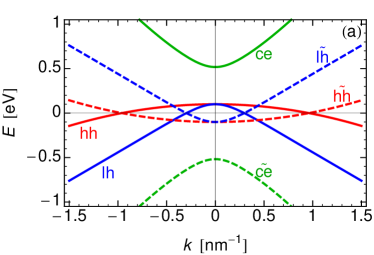
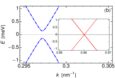
The characteristics of the proximity effect induced in the valence band via coupling to the conduction band are illustrated in Fig. 1. We plot dispersions of relevant energy bands obtained from the $12\times 12$ BdG Hamiltonian in Eq. (1), with band-structure parameters applicable for InAs Vurgaftman et al. (2001); Winkler (2003). To set the scene, Fig. 1(a) shows the result for $\Delta=0$, where conduction-electron states (ce), light-hole states (lh) and heavy-hole states (hh) are decoupled from their corresponding time-reversed states (denoted by $\widetilde{\text{ce}}$, $\widetilde{\text{lh}}$ and $\widetilde{\text{hh}}$, respectively). Figure. 1(b) zooms in on the valence-band dispersions in the vicinity of the Fermi level when $\Delta=1$ meV. In agreement with (28), an energy gap is found for the LH-like states and, in the vicinity of the Fermi level, the LH-like quasiparticle states are linear combinations of normal excitations (ce and lh) and time-reversed partners ($\widetilde{\text{ce}}$ and $\widetilde{\text{lh}}$). In contrast, no gap appears for the HH states. Thus, in summary, the proximity effect in bulk-hole systems can be understood in terms of the familiar decoupled HH and LH excitations, with HHs being unaffected and LHs experiencing superconductivity with an $s$-wave type pairing that, to leading order, depends quadratically on wave vector ($\Delta_{\frac{1}{2},-\frac{1}{2}}\propto|{\bm{\mathrm{k}}}|^{2}$).

IV.2 Quasi-twodimensional (quantum-well) systems

A quantum-well confinement of electrons in the semiconductor structure can be treated by replacing $\mathsf{H}_{\text{v}}^{(\text{eff})}\to\mathsf{H}_{\text{v}}^{(\text{eff})}+V(z)$ in Eq. (20). Subband-${\bm{\mathrm{k}}}$dot${\bm{\mathrm{p}}}$ theory Broido and Sham (1985); Yang et al. (1985) could then be applied to find the energy dispersions and the corresponding eigenstates. To get a qualitative insight into the proximity effect for quasi-twodimensional (quasi-2D) hole systems, we treat the confining potential in an approximate manner Kernreiter et al. (2010) by setting $k_{z}\to 0$ and $k_{z}^{2}\to n^{2}\pi^{2}/d^{2}$ in the bulk-hole BdG Hamiltonian, Eq. (20). Here $d$ denotes the effective quantum-well width, and $n=1,2,\dots$ labels orbital bound states associated with the quantum-well potential $V(z)$. Such a procedure renders the valence-band BdG Hamiltonian block-diagonal for each $n$, with $2\times 2$ blocks in the subspaces $\{3/2,-1/2\}$ and $\{-3/2,1/2\}$ labelled by the index $\sigma=\pm 1$:

$${\mathcal{H}}_{\text{BdG}}^{(\text{eff},\text{2D})}=\bigotimes_{\dots n=1,2,\atop\sigma=\pm 1}\begin{pmatrix}\mathsf{H}_{\sigma,n}^{(\text{2D})}-\mu\,\openone_{2\times 2}&\Delta_{\sigma,n}^{(\text{2D})}\\ \left(\Delta_{\sigma,n}^{(\text{2D})}\right)^{\dagger}&\mu\,\openone_{2\times 2}-\mathsf{H}_{\sigma,n}^{(\text{2D})}\end{pmatrix}.$$ (29)

Defining ${\bm{\mathrm{k}}}_{\perp}=(k_{x},k_{y})$ and adopting the spherical approximation for the Luttinger model Suzuki and Hensel (1974); Trebin et al. (1979), the sub-matrices are given by

$$\mathsf{H}_{\sigma,n}^{(\text{2D})} = \begin{pmatrix}E_{n}^{(\text{h})}-\frac{\hbar^{2}k_{\perp}^{2}}{2m_{\perp}^{(\text{h})}}&\frac{\sqrt{3}\gamma_{3}\hbar^{2}k_{-\sigma}^{2}}{2m_{0}}\\ \frac{\sqrt{3}\gamma_{3}\hbar^{2}k_{\sigma}^{2}}{2m_{0}}&E_{n}^{(\text{l})}-\frac{\hbar^{2}k_{\perp}^{2}}{2m_{\perp}^{(\text{l})}}\end{pmatrix}\,\,,$$ (30a)

$$\Delta_{\sigma,n}^{(\text{2D})} = \Delta\,\frac{\bar{\gamma}_{1}\hbar^{2}}{2m_{0}E_{\text{g}}}\begin{pmatrix}\frac{3k_{\perp}^{2}}{2}&-\frac{\sqrt{3}k_{-\sigma}^{2}}{2}\\[5.69046pt] -\frac{\sqrt{3}k_{\sigma}^{2}}{2}&\frac{2\pi^{2}n^{2}}{d^{2}}+\frac{k_{\perp}^{2}}{2}\,\end{pmatrix}\,\,,$$ (30b)

where $E_{n}^{(\text{h/l})}$ are quasi-2D subband energies for HH/LH states at ${\bm{\mathrm{k}}}_{\perp}=0$, and $m_{\perp}^{(\text{h/l})}$ their respective effective masses for the in-plane motion. For a $(001)$ quantum well, these effective masses are $m_{\perp}^{(\text{h/l})}=m_{0}/(\gamma_{1}\pm\gamma_{2})$ in terms of the standard Vurgaftman et al. (2001) Luttinger parameters.

For the sake of completeness, we have given the expressions of the sub-matrices Eqs. (30) for an arbitrary value of the orbital bound-state index $n$. However, it should be noted that the results are reliable only for the lowest subband, i.e., $n=1$. The Hamiltonian (29) together with Eqs. (30) is the central result of this section; it provides a simple model to describe proximity-induced superconductivity in quasi-2D hole systems in the low-density regime (such that only one quantum-well subband is occupied).

Figure 2: Effective superconducting pair potentials of quasi-2D holes. The result for HH-like (LH-like) excitations in the $n=1$ quantum-well bound state, i.e., the lowest (first excited) subband, is shown as the blue solid (red dashed) curve. See also Eq. (31b). The different scales for $\Delta^{(+)}_{1}$ (blue/left ordinate) and $\Delta^{(-)}_{1}$ (red/right ordinate) emphasize the different band widths in the ${\bm{\mathrm{k}}}$-dependence for pair potentials of HH-like and LH-like excitations, as well as the absence/existence of a constant contribution. Band-structure parameters have been absorbed into the definition of $\Delta^{(2\text{D})}_{0}\equiv\pi^{2}\bar{\gamma}_{1}\hbar^{2}\Delta/(2m_{0}d^{2}E_{\text{g}})$.

To make contact with the usual intuition about superconducting correlations, we perform a unitary transformation of ${\mathcal{H}}_{\text{BdG}}^{(\text{eff},\text{2D})}$ that diagonalizes the pair-potential matrices $\Delta_{\sigma,n}^{(\text{2D})}$. Straightforward calculation yields

$$\tilde{\Delta}_{\sigma,n}^{(\text{2D})}\equiv{\mathcal{U}}\,\Delta_{\sigma,n}^{(\text{2D})}\,{\mathcal{U}}^{\dagger}=\begin{pmatrix}\Delta_{n}^{(+)}&0\\ 0&\Delta_{n}^{(-)}\end{pmatrix}\,\,,$$ (31a)

where (using $$\kappa:=k_{\perp}d/\pi$$)

$$\Delta_{n}^{(\pm)}=\Delta\,\frac{\pi^{2}\bar{\gamma}_{1}\hbar^{2}}{2m_{0}d^{2}E_{\text{g}}}\left(n^{2}+\kappa^{2}\mp\sqrt{n^{4}-\kappa^{2}+\kappa^{4}}\right)\,.$$ (31b)

Note the limiting behavior for $\kappa\ll 1$:

$$\Delta_{n}^{(+)} \to \Delta\,\frac{3\bar{\gamma}_{1}\hbar^{2}k_{\perp}^{2}}{4m_{0}E_{\text{g}}}\leavevmode\nobreak\ ,$$ (32a)

$$\Delta_{n}^{(-)} \to \Delta\,\frac{\pi^{2}\bar{\gamma}_{1}\hbar^{2}n^{2}}{m_{0}d^{2}E_{\text{g}}}\left[1+\left(\frac{k_{\perp}d}{2\pi}\right)^{2}\right]\leavevmode\nobreak\ .$$ (32b)

In Fig. 2, we plot the induced pair potentials from Eq. (31b) as a function of $k_{\perp}d/\pi$. As the same transformation that diagonalizes $\Delta_{\sigma,n}^{(\text{2D})}$ also renders $\mathsf{H}_{\sigma,n}^{(\text{2D})}$ to be diagonal within the spherical approximation, we find that the effective pair potential for quasiparticles from the HH-like quasi-2D hole subbands is $k_{\perp}$-dependent (i.e, does not vanish as was the case for HH states in the bulk) and can thus strongly increase with variation of the quasi-2D hole density. Also unlike their bulk counterparts, the LH-like quasi-2D hole states are subject to a pair potential that is, to leading order, a constant. In particular, states at the Fermi energy in the lowest subband, which is HH-like, will have a density-dependent superconducting gap that scales linearly with the quasi-2D hole density. Except at ${\bm{\mathrm{k}}}_{\perp}=0$, the quasiparticle states arising from superconducting correlations are mixtures of HH and LH states. State-dependent physical quantities such as response functions will be affected by this HH-LH mixing, reflecting the spinor structure of confined hole states Kernreiter et al. (2010, 2013a); Kernreiter (2013); Kernreiter et al. (2013b).

IV.3 Quasi-onedimensional (nanowire) systems

We consider hole nanowires defined by a transverse hard-wall confinement for two distinct sample geometries: 1) a system with rectangular cross-section, which can serve as a model for quantum wires obtained by electrostatic confinement of a 2D hole gas Srinivasan et al. (2013), and 2) a cylindrical nanowire that can be fabricated, e.g., by the VLS growth method Lu and Lieber (2006).

IV.3.1 Quantum wire with rectangular cross-section

We first consider the holes to be confined in a rectangular quasi-1D system by a hard-wall confinement with potential $V(x,y)=V(x)V(y)$, where the quantum-well widths in $x$ and $y$ directions are $d$ and $w$, respectively. We use again an approximation, setting $k_{x},k_{y}\to 0$ and $k_{x}^{2}\to n^{2}\pi^{2}/d^{2}$ and $k_{y}^{2}\to n^{\prime 2}\pi^{2}/w^{2}$. Similarly to Eq. (29), the corresponding BdG Hamiltonian is then block-diagonal, with associated $2\times 2$ sub-matrices

$$\mathsf{H}_{\sigma,nn^{\prime}}^{(\text{1D})} =$$

$$\begin{pmatrix}-\frac{\pi^{2}\hbar^{2}(n^{2}+r^{2}n^{\prime 2})}{2m_{\perp}^{(\text{h})}d^{2}}-\frac{\hbar^{2}k_{z}^{2}}{2m_{\|}^{(\text{h})}}&\frac{\sqrt{3}\gamma_{3}\pi^{2}\hbar^{2}(n^{2}-r^{2}n^{\prime 2})}{2m_{0}d^{2}}\\ \frac{\sqrt{3}\gamma_{3}\pi^{2}\hbar^{2}(n^{2}-r^{2}n^{\prime 2})}{2m_{0}d^{2}}&-\frac{\pi^{2}\hbar^{2}(n^{2}+r^{2}n^{\prime 2})}{2m_{\perp}^{(\text{l})}d^{2}}-\frac{\hbar^{2}k_{z}^{2}}{2m_{\|}^{(\text{l})}}\end{pmatrix},\quad$$

$$\Delta_{\sigma,nn^{\prime}}^{(\text{1D})} = \Delta\,\frac{\pi^{2}\bar{\gamma}_{1}\hbar^{2}}{2m_{0}d^{2}E_{\text{g}}}$$ (33b)

$$\times\begin{pmatrix}\frac{3}{2}(n^{2}+r^{2}n^{\prime 2})&-\frac{\sqrt{3}}{2}(n^{2}-r^{2}n^{\prime 2})\\[5.69046pt] -\frac{\sqrt{3}}{2}(n^{2}-r^{2}n^{\prime 2})&\frac{1}{2}(1+r^{2})+2\kappa_{z}^{2}\,\end{pmatrix},$$

where $\kappa_{z}\equiv k_{z}d/\pi$, $r\equiv d/w$, and $m_{\|}^{(\text{h/l})}$ are the effective masses for HH/LH motion parallel to the spin-3/2 quantization axis. [For example, $m_{\|}^{(\text{h/l})}=m_{0}/(\gamma_{1}\mp 2\gamma_{2})$ when the quantization axis is parallel to the $(001)$ crystallographic direction.] The index $\sigma=\pm$ distinguishes the subspaces $\{3/2,-1/2\}$ and $\{-3/2,1/2\}$, respectively. From now on, we focus on the lowest quasi-1D hole subband, which has $n=n^{\prime}=1$. Diagonalizing Eq. (33b) yields the induced superconducting pair potential for this system,

$$\Delta^{(\pm)} = \Delta\,\frac{\pi^{2}\bar{\gamma}_{1}\hbar^{2}}{2m_{0}d^{2}E_{\text{g}}}\left(1+r^{2}+\kappa_{z}^{2}\right.$$ (34)

$$\hskip 14.22636pt\left.\mp\sqrt{1-r^{2}+r^{4}-\kappa_{z}^{2}(1+r^{2})+\kappa_{z}^{4}}\right)\,.$$

We recover the 2D result of Eq. (31b) for $r\to 0$, with $k^{2}_{\perp}$ replaced by $k^{2}_{z}$. For the symmetric case $r=1$, we obtain

$$\left.\Delta^{(+)}\right|_{r=1} = \Delta\,\frac{\pi^{2}\bar{\gamma}_{1}\hbar^{2}}{2m_{0}d^{2}E_{\text{g}}}\left[1+2\left(\frac{k_{z}\pi}{d}\right)^{2}\right],$$ (35a)

$$\left.\Delta^{(-)}\right|_{r=1} = \Delta\,\frac{3\pi^{2}\bar{\gamma}_{1}\hbar^{2}}{2m_{0}d^{2}E_{\text{g}}}\,\,.$$ (35b)

Again we find a nontrivial dependence of the induced superconducting pair potential with respect to the hole density (quadratically dependent on the quantum wire hole density) for the lowest subband, which is LH-like (for $r=1$) due to the phenomenon of mass inversion, i.e., since $m_{\perp}^{(\text{h})}<m_{\perp}^{(\text{l})}$.

IV.3.2 Quantum wire with circular cross-section

Next we consider a quasi-onedimensional (quasi-1D) system with cylindrical geometry. In this case, it is convenient to use cylindrical coordinates $(r,\varphi,z)$. A hard-wall confinement is imposed by a potential $V(r)$ defined by $V(r)=0$ for $r<R$ and $V(r)=\infty$ for $r>R$, where $R$ is the radius of the cylindrical wire. Due to the cylindrical symmetry of the system, the Hamiltonian commutes with the projection of total angular momentum parallel to the nanowire (i.e., the $z$) axis. Therefore the eigenstates of the Hamiltonian can be classified Sercel and Vahala (1990) by the eigenvalue $\nu$ of $F_{z}=-i\partial_{\varphi}+J_{z}$. Using the appropriate representation, we find the eigenfunctions at the subband edge by solving the purely transverse bound-state problem ($k_{z}=0$). For $k_{z}=0$ the subspaces $\{3/2,-1/2\}$ and $\{-3/2,1/2\}$ labelled by the index $\sigma=\pm 1$ are decoupled, while for finite $k_{z}$ this is no longer the case. We denote the subband-edge eigenfunctions by $\Psi^{(0)}_{(\sigma,\nu,n)}$, where the index $n$ labels the different radial quasi-1D states associated to given values of $\sigma$ and $\nu$. The ground state is doubly degenerate and, for wires made from InAs,  the two states have quantum numbers $\sigma=\pm 1,\nu=\pm 1/2,n=1$, hence the corresponding wave functions for $k_{z}=0$ are $\Psi^{(0)}_{(1,\frac{1}{2},1)}$ and $\Psi^{(0)}_{(-1,-\frac{1}{2},1)}$. The first excited subband is also doubly degenerate ($\sigma=\pm 1,\nu=\mp 1/2,n=1$), and the wave functions are $\Psi^{(0)}_{(-1,\frac{1}{2},1)}$ and $\Psi^{(0)}_{(1,-\frac{1}{2},1)}$. More details about the calculation of the cylindrical-hole-nanowire subbands are given in the Appendix.

We project the nanowire Hamiltonian and pair potential onto the subspace of the two lowest subband-edge states Sercel and Vahala (1990); Csontos et al. (2009); Kloeffel et al. (2011). Since $\nu$ is a conserved quantum number, the resulting Hamiltonian is block diagonal in the two subspaces spanned by $\{\Psi^{(0)}_{(1,\frac{1}{2},1)},\Psi^{(0)}_{(-1,\frac{1}{2},1)}\}$ and $\{\Psi^{(0)}_{(-1,-\frac{1}{2},1)},\Psi^{(0)}_{(1,-\frac{1}{2},1)}\}$. In each of the subspaces, the effective BdG Hamiltonian for the cylindrical quantum wire reads

$$\mathsf{H}_{\text{cyl}}^{(\text{1D})} = -\frac{\hbar^{2}\gamma_{1}}{2m_{0}R^{2}}\begin{pmatrix}\tilde{E}^{(\text{g})}+\frac{(k_{z}R)^{2}}{\tilde{m}^{(\text{g})}}&iCk_{z}R\\ -iCk_{z}R&\tilde{E}^{(\text{e})}+\frac{(k_{z}R)^{2}}{\tilde{m}^{(\text{e})}}\end{pmatrix},$$

$$\Delta_{\text{cyl}}^{(\text{1D})} = \frac{3\Delta\hbar^{2}\bar{\gamma}_{1}}{2m_{0}R^{2}E_{\text{g}}}\begin{pmatrix}\frac{(k_{z}R)^{2}}{2}&iDk_{z}R\\ -iDk_{z}R&\tilde{\Delta}+\frac{(k_{z}R)^{2}}{\tilde{m}^{(\Delta)}}\end{pmatrix}\,.$$ (36b)

For an InAs nanowire, the parameters entering Eqs. (36) and (36b) are $\tilde{E}^{(\text{g})}=1.47$, $\tilde{E}^{(\text{e})}=2.23$, $\tilde{m}^{(\text{g})}=0.69$, $\tilde{m}^{(\text{e})}=0.61$, $C=0.69$, $\tilde{\Delta}=0.22$, $\tilde{m}^{(\Delta)}=1.74$, and $D=0.26$. Diagonalization of Eq. (36b) yields the induced superconducting pair potential of hole-nanowire states to read

$$\Delta_{\text{cyl}}^{(1,2)}=\frac{3\bar{\gamma}_{1}\hbar^{2}\Delta}{8m_{0}R^{2}E_{\text{g}}}\left\{2\tilde{\Delta}+(k_{z}R)^{2}\left(1+\frac{2}{\tilde{m}^{(\Delta)}}\right)\mp\sqrt{4\tilde{\Delta}^{2}+4(k_{z}R)^{2}\tilde{\Delta}\left(\frac{2}{\tilde{m}^{(\Delta)}}-1+\frac{4D^{2}}{\tilde{\Delta}}\right)+(k_{z}R)^{4}\left(1-\frac{2}{\tilde{m}^{(\Delta)}}\right)^{2}}\right\}.$$ (37)

In the limit $k_{z}R\ll 1$, we find

$$\Delta_{\text{cyl}}^{(1)} \to \Delta\,\frac{3\bar{\gamma}_{1}\hbar^{2}}{2m_{0}E_{\text{g}}}\left(\frac{1}{2}-\frac{D^{2}}{\tilde{\Delta}}\right)k_{z}^{2}\leavevmode\nobreak\ ,$$ (38a)

$$\Delta_{\text{cyl}}^{(2)} \to \Delta\,\frac{3\bar{\gamma}_{1}\hbar^{2}}{2m_{0}R^{2}E_{\text{g}}}\left[\tilde{\Delta}+\left(\frac{1}{\tilde{m}^{(\Delta)}}+\frac{D^{2}}{\tilde{\Delta}}\right)\left(k_{z}R\right)^{2}\right]\leavevmode\nobreak\ .$$

The states that are directly coupled by the superconducting pair potential turn out to be mixtures of the two lowest-lying nanowire-subband states. The wave-vector dependence of proximity-induced gap parameters is displayed in Fig. 3. It mirrors qualitatively the behavior of quantum-well states [cf. Eqs. (31b) and (32)], which is a point of difference with the rectangular-wire case. In particular, the pair potential for lowest-subband-dominated states in a cylindrical InAs wire is finite only when $k_{z}\neq 0$ and, therefore, strongly density-tunable. We note that the effective Hamiltonian in Eq. (36) and the effective gap matrix, Eq. (36b), cannot be simultaneously diagonalized in general.

Figure 3: Effective superconducting pair potentials of quasi-1D hole states in a cylindrical nanowire. See Eq. (37). In the limit of small $k_{z}R$, the blue solid (red dashed) curve is associated with eigenstates from the lowest (first excited) nanowire subband. In general, the states that are directly coupled by these pair potentials are superpositions of eigenstates at the same $k_{z}$ from the lowest two subbands. We assumed band-structure parameters for InAs and defined $\Delta^{(1\text{D})}_{0}\equiv\bar{\gamma}_{1}\hbar^{2}\Delta/(2m_{0}E_{\text{g}}R^{2})$.

V Summary and Conclusions

We have developed a general theoretical description of the superconducting proximity effect for charge carriers from a semiconductor’s valence band arising from coupling to a simple-metal superconductor. Our starting point is an s-wave pair potential that is induced for conduction electrons by means of the ordinary proximity effect de Gennes (1964); Volkov et al. (1995); Fagas et al. (2005); Kopnin and Melnikov (2011). We show how the familiar inter-band coupling yields an unusual proximity effect for holes, with induced pair potentials depending strongly on the dimensionality of the p-doped system. In particular, in a bulk sample, only light-hole state are subject to a finite pair potential, which depends quadratically on wave vector. A rich behavior is revealed for quantum-confined holes, with intriguing parallels being exhibited by quasi-2D (quantum-well) systems and cylindrically shaped quantum wires made from InAs. See Figures 2 and 3. In both of these cases, the pair potential couples states that are mixtures between heavy-hole and light-hole components. The pair potential affecting the lowest-lying subband states (shown as the blue solid curve in both figures) is proportional to the squared magnitude of the hole wave vector and, therefore, strongly tunable by the carrier density. In marked contrast to the bulk case, the pair potential for quantum-confined holes can also have a constant contribution as is exhibited by the first excited subbands (see the red dashed curve in both figures).

The wave-vector dependence of induced pair potentials for holes enables direct tuning of superconducting correlations and gap parameters in these systems. This previously unnoticed feature renders confined hole systems ideal laboratories for investigating the transition to, and properties of, novel topological phases with their associated unconventional quasiparticle excitations Alicea (2012); Leijnse and Flensberg (2012); Beenakker (2013); Stanescu and Tewari (2013). However, the influence of the, so far unappreciated, fact that the pair-potential-coupled states are generally mixtures of heavy-hole and light-hole contributions requires further detailed study. Also, a deeper understanding of the effect of Rashba-type spin-orbit coupling and magnetic-field-induced spin splittings in conjunction with the unconventional properties of proximity-induced superconductivity in hole systems needs to be developed.

*

Appendix A Luttinger-model description of cylindrical hole nanowires defined by a hard-wall potential

To take full advantage of the cylindrical symmetry of the nanowire, we adopt the cylindrical coordinates $(r,\varphi,z)$. The wire is described by the Schrödinger equation $\left[\mathsf{H}_{\text{v}}^{(\text{eff})}+V(r)\right]\Psi({\bm{\mathrm{r}}})=E\,\Psi({\bm{\mathrm{r}}})$. Within the axial approximation for the Luttinger Hamiltonian $\mathsf{H}_{\text{v}}^{(\text{eff})}$, the Ansatz

$$\Psi({\bm{\mathrm{r}}})=\mathrm{e}^{ik_{z}z}\,\,\mathrm{e}^{i\left(\nu-J_{z}\right)\varphi}\,\,\Phi_{\nu}^{(k_{z})}(r)$$ (39)

transforms the original 3D Schrödinger problem for the nanowire into a 1D radial equation $\left[\bar{\mathsf{H}}_{\nu}(k_{z})+V(r)\right]\Phi_{\nu}^{(k_{z})}(r)=E_{\nu}(k_{z})\,\Phi_{\nu}^{(k_{z})}(r)$. Here $\nu$ is the quantum number associated with the total angular momentum component parallel to the wire axis, which is given by $F_{z}=-i\partial_{\varphi}+J_{z}$.

In the spirit of subband ${\bm{\mathrm{k}}}$dot${\bm{\mathrm{p}}}$ theory, we separate the effective radial-motion Hamiltonian into two parts, $\bar{\mathsf{H}}_{\nu}(k_{z})=\bar{\mathsf{H}}_{\nu}^{(0)}+\bar{\mathsf{H}}_{\nu}^{(1)}(k_{z})$, where $\bar{\mathsf{H}}_{\nu}^{(0)}\equiv\bar{\mathsf{H}}_{\nu}(k_{z}=0)$. Straightforward calculation yields

$$\bar{\mathsf{H}}_{\nu}^{(0)} = -\frac{\hbar^{2}}{2m_{0}}\left\{\left[\gamma_{1}+\gamma_{2}\left(J_{z}^{2}-\frac{5}{4}\,\openone\right)\right]{\bm{\mathrm{k}}}_{\|\nu}^{2}+\gamma_{3}\left(J_{+}^{2}\,L_{\nu-1}\,L_{\nu}+J_{-}^{2}\,L_{\nu+2}^{\dagger}\,L_{\nu+1}^{\dagger}\right)\right\},$$ (40a)

$$\bar{\mathsf{H}}_{\nu}^{(1)}(k_{z}) = -\frac{\hbar^{2}}{2m_{0}}\left\{\left[\gamma_{1}-2\gamma_{2}\left(J_{z}^{2}-\frac{5}{4}\,\openone\right)\right]k_{z}^{2}+2\sqrt{2}\,\gamma_{2}\,i\left(\{J_{+}\,,\,J_{z}\}\,L_{\nu}-\{J_{-}\,,\,J_{z}\}\,L_{\nu+1}^{\dagger}\right)k_{z}\right\}.$$ (40b)

Here we have used the abbreviations

$${\bm{\mathrm{k}}}_{\|\nu} = -\partial_{r}^{2}-\frac{1}{r}\,\partial_{r}+\frac{\left(\nu-J_{z}\right)^{2}}{r^{2}}\quad,$$ (41a)

$$L_{\nu} = \partial_{r}+\frac{\nu-J_{z}}{r}\,\,,\,\,L_{\nu}^{\dagger}=-\partial_{r}+\frac{\nu-1-J_{z}}{r}\,.\quad$$ (41b)

In the following, we adopt the spherical approximation, i.e. $\gamma_{2}=\gamma_{3}\equiv\gamma_{\text{s}}=(2\gamma_{2}+3\gamma_{3})/5$. We first consider the purely transverse motion, i.e. $k_{z}=0$.

Straightforward inspection shows that $\bar{\mathsf{H}}_{\nu}^{(0)}$ is block-diagonal in the subspaces spanned by intrinsic angular-momentum projections $\{\pm 3/2,\mp 1/2\}$, labelled by $\sigma=\pm 1$. Therefore we can solve the transverse problem independently for each value of $\sigma$. For this the transverse Schrödinger equation reads

$$\left[\bar{\mathsf{H}}_{\nu}^{(0)}+V(r)\right]\Phi^{(0)}_{\sigma,\nu,n}(r)=E_{\sigma,\nu,n}(0)\,\Phi^{(0)}_{\sigma,\nu,n}(r)\quad,$$ (42)

where the index $n=1,2,\dots$ labels in order of ascending energies the different quasi-1D subbands for given values of $\sigma$ and $\nu$. Without confinement, the eigenstates for the Hamiltonian (40a) are found to be

$$\phi_{1,\nu,\pm}(r)=\left(a_{\pm}\,J_{\nu-\frac{3}{2}}(k_{\pm}r),0,c_{\pm}\,J_{\nu+\frac{1}{2}}(k_{\pm}r),0\right)^{T},$$ (43a)

$$\phi_{-1,\nu,\pm}(r)=\left(0,b_{\pm}\,J_{\nu-\frac{1}{2}}(k_{\pm}r),0,d_{\pm}\,J_{\nu+\frac{3}{2}}(k_{\pm}r)\right)^{T},$$ (43b)

where $k_{\pm}=\sqrt{2m_{0}/(\hbar^{2}\gamma_{1})}\sqrt{m_{\pm}|E|}$ with $E$ being the energy, $m_{\pm}=1/(1\mp 2\bar{\gamma})$, $\bar{\gamma}=\gamma_{\text{s}}/\gamma_{1}$, and coefficients $a_{\pm}=\{-1,\sqrt{3}\}$, $b_{\pm}=\{-\sqrt{3},1\}$, $c_{\pm}=\{\sqrt{3},1\}$ and $d_{\pm}=\{1,\sqrt{3}\}$. In Eqs. (43), Bessel functions of the first kind (denoted by $J_{M}$) have been introduced. In the following, we assume a quantum wire to be fabricated from InAs with the appropriate values for the band structure parameters, which implies $\bar{\gamma}=0.45$. (The materials dependence of valence-band states confined to cylindrical nanowires has been discussed in Ref. Zülicke and Csontos, 2008.) The quantum-wire bound states are written as a superposition of 2D states with the same value of $\sigma$, that is

$$\Phi_{\sigma,\nu,n}^{(0)}(r)=\frac{1}{R}\left[a_{\sigma,\nu,n}\phi_{\sigma,\nu,+}(r)+b_{\sigma,\nu,n}\phi_{\sigma,\nu,-}(r)\right],$$ (44)

with $\sigma=1$ or $-1$. The eigenergies are obtained by imposing the proper boundary condition at $r=R$. This amounts to solving the secular equation

$$J_{\nu-\frac{3}{2}}(k_{+}R)J_{\nu+\frac{1}{2}}(k_{-}R)+3J_{\nu+\frac{1}{2}}(k_{+}R)J_{\nu-\frac{3}{2}}(k_{-}R)=0$$ (45)

for $\sigma=1$ and

$$J_{\nu+\frac{3}{2}}(k_{+}R)J_{\nu-\frac{1}{2}}(k_{-}R)+3J_{\nu-\frac{1}{2}}(k_{+}R)J_{\nu+\frac{3}{2}}(k_{-}R)=0$$

for $\sigma=-1$. We find that the lowest subbands are the ones where ($\sigma=1,\nu=\frac{1}{2},n=1$) and ($\sigma=-1,\nu=-\frac{1}{2},n=1$). The associated bound state energy is $|\varepsilon^{(1)}|=1.47\,\varepsilon_{0}$ [with $\varepsilon_{0}=\hbar^{2}\gamma_{1}/(2m_{0}R^{2})$], and the coefficients are $a_{-1,-1/2,1}=-a_{1,1/2,1}=0.70$ and $b_{1,1/2,1}=b_{-1,-1/2,1}=0$, where the normalization condition for the wave function has been included.

The first excited subbands are the ones where $(\sigma=1,\nu=-\frac{1}{2},n=1)$ and $(\sigma=-1,\nu=\frac{1}{2},n=1)$. The corresponding bound-state energy is $|\varepsilon^{(2)}|=2.23\,\varepsilon_{0}$. For the excited subbands, we find $a_{1,-1/2,1}=-a_{-1,1/2,1}=0.693$ and $b_{1,-1/2,1}=b_{-1,1/2,1}=0.436$.

The wave functions for the lowest subbands and first excited subbands are thus given by

$$\Psi^{(0)}_{(1,\frac{1}{2},1)}(r,\varphi) = \mathrm{e}^{i(\frac{1}{2}-J_{z})\varphi}\leavevmode\nobreak\ \Phi_{1,\frac{1}{2},1}^{(0)}(r)\leavevmode\nobreak\ ,$$ (47a)

$$\Psi^{(0)}_{(-1,-\frac{1}{2},1)}(r,\varphi) = \mathrm{e}^{-i(\frac{1}{2}+J_{z})\varphi}\leavevmode\nobreak\ \Phi_{-1,-\frac{1}{2},1}^{(0)}(r)\leavevmode\nobreak\ ,$$ (47b)

and

$$\Psi^{(0)}_{(1,-\frac{1}{2},1)}(r,\varphi) = \mathrm{e}^{-i(\frac{1}{2}+J_{z})\varphi}\leavevmode\nobreak\ \Phi_{1,-\frac{1}{2},1}^{(0)}(r)\leavevmode\nobreak\ ,$$ (48a)

$$\Psi^{(0)}_{(-1,\frac{1}{2},1)}(r,\varphi) = \mathrm{e}^{i(\frac{1}{2}-J_{z})\varphi}\leavevmode\nobreak\ \Phi_{-1,\frac{1}{2},1}^{(0)}(r)\leavevmode\nobreak\ ,$$ (48b)

respectively.

The effective Hamiltonian of the cylindrical hole quantum wire for $k_{z}\neq 0$ is obtained by projection in the subspace spanned by states from Eqs. (47a)-(48b):

$$\langle\Psi^{(0)}_{(\sigma^{\prime},\nu,n^{\prime})}|\mathsf{H}_{\text{v}}^{(\text{eff})}|\Psi^{(0)}_{(\sigma,\nu,n)}\rangle\leavevmode\nobreak\ ,$$ (49)

where the inner product is $\langle\cdots\rangle=\int_{0}^{R}drr\int_{0}^{2\pi}d\varphi\cdots$. The matrix of the superconducting pair potential can be obtained straightforwardly by first transforming the matrix in Eq. (21) into cylindrical coordinates and then calculating the matrix elements with respect to the basis states in Eqs. (47a)-(48b).

References

• Hekking et al. (1994) F. W. J. Hekking, G. Schön,  and D. V. Averin, eds., Mesoscopic Superconductivity (Elsevier Science, Amsterdam, 1994) special issue of Physica B 203.
• (2) C. W. J. Beenakker, “Quantum Transport in Semiconductor-Superconductor Microjunctions,” in Ref. Akkermans et al., 1995, pp. 279-324.
• (3) B. J. van Wees and H. Takayanagi, “The Superconducting Proximity Effect in Semiconductor-Superconductor Systems: Ballistic Transport, Low Dimensionality and Sample Specific Properties,” in Ref. Sohn et al., 1997, pp. 469–501.
• Lambert and Raimondi (1998) C. J. Lambert and R. Raimondi, J. Phys.: Condens. Matter 10, 901 (1998).
• Schäpers (2001) T. Schäpers, Superconductor/Semiconductor Junctions (Springer, Berlin, 2001).
• Takayanagi et al. (2008) H. Takayanagi, J. Nitta,  and H. Nakano, eds., Controllable Quantum States: Mesoscopic Superconductivity and Spintronics (World Scientic, Singapore, 2008).
• Akkermans et al. (1995) E. Akkermans, G. Montambeaux, J.-L. Pichard,  and J. Zinn-Justin, eds., Mesoscopic Quantum Physics, Proceedings of the 1994 Les Houches Summer School, Session LXI (Elsevier Science, Amsterdam, 1995).
• Sohn et al. (1997) L. L. Sohn, L. P. Kouwenhoven,  and G. Schön, eds., Mesoscopic Electron Transport, NATO ASI Series E, Vol. 345 (Kluwer Academic, Dordrecht, 1997).
• Beenakker (1997) C. W. J. Beenakker, Rev. Mod. Phys. 69, 731 (1997).
• de Gennes (1964) P. G. de Gennes, Rev. Mod. Phys. 36, 225 (1964).
• Volkov et al. (1995) A. F. Volkov, P. H. C. Magnée, B. J. van Wees,  and T. M. Klapwijk, Physica C 242, 261 (1995).
• Fagas et al. (2005) G. Fagas, G. Tkachov, A. Pfund,  and K. Richter, Phys. Rev. B 71, 224510 (2005).
• Kopnin and Melnikov (2011) N. B. Kopnin and A. S. Melnikov, Phys. Rev. B 84, 064524 (2011).
• Lutchyn et al. (2010) R. M. Lutchyn, J. D. Sau,  and S. Das Sarma, Phys. Rev. Lett. 105, 077001 (2010).
• Oreg et al. (2010) Y. Oreg, G. Refael,  and F. von Oppen, Phys. Rev. Lett. 105, 177002 (2010).
• Sau et al. (2010) J. D. Sau, R. M. Lutchyn, S. Tewari,  and S. Das Sarma, Phys. Rev. Lett. 104, 040502 (2010).
• Alicea (2010) J. Alicea, Phys. Rev. B 81, 125318 (2010).
• Klinovaja et al. (2012) J. Klinovaja, P. Stano,  and D. Loss, Phys. Rev. Lett. 109, 236801 (2012).
• Zyuzin et al. (2013) A. A. Zyuzin, D. Rainis, J. Klinovaja,  and D. Loss, Phys. Rev. Lett. 111, 056802 (2013).
• Alicea (2012) J. Alicea, Rep. Prog. Phys. 75, 076501 (2012).
• Leijnse and Flensberg (2012) M. Leijnse and K. Flensberg, Semicond. Sci. Technol. 27, 124003 (2012).
• Beenakker (2013) C. Beenakker, Annu. Rev. Condens. Matter Phys. 4, 113 (2013).
• Stanescu and Tewari (2013) T. D. Stanescu and S. Tewari, J. Phys.: Condens. Matter 25, 233201 (2013).
• Winkler (2003) R. Winkler, Spin-Orbit Coupling Effects in Two-Dimensional Electron and Hole Systems (Springer, Berlin, 2003).
• Kloeffel et al. (2011) C. Kloeffel, M. Trif,  and D. Loss, Phys. Rev. B 84, 195314 (2011).
• Mao et al. (2011) L. Mao, J. Shi, Q. Niu,  and C. Zhang, Phys. Rev. Lett. 106, 157003 (2011).
• Mao et al. (2012) L. Mao, M. Gong, E. Dumitrescu, S. Tewari,  and C. Zhang, Phys. Rev. Lett. 108, 177001 (2012).
• Yu and Cardona (2010) P. Y. Yu and M. Cardona, Fundamentals of Semiconductors, 4th ed. (Springer, Berlin, 2010).
• Kane (1957) E. O. Kane, J. Phys. Chem. Solids 1, 249 (1957).
• Futterer et al. (2011) D. Futterer, M. Governale, U. Zülicke,  and J. König, Phys. Rev. B 84, 104526 (2011).
• Andreev (1964) A. F. Andreev, Zh. Eksp. Teor. Fiz. 46, 1823 (1964), [Sov. Phys. JETP 19, 1228 (1964)].
• de Gennes and Saint-James (1963) P. G. de Gennes and D. Saint-James, Phys. Lett. 4, 151 (1963).
• de Gennes (1989) P. G. de Gennes, Superconductivity of Metals and Alloys (Addison-Wesley, Reading, MA, 1989).
• Foldy and Wouthuysen (1950) L. L. Foldy and S. A. Wouthuysen, Phys. Rev. 78, 29 (1950).
• Löwdin (1951) P.-O. Löwdin, J. Chem. Phys. 19, 1396 (1951).
• Luttinger (1956) J. M. Luttinger, Phys. Rev. 102, 1030 (1956).
• Lipari and Baldereschi (1970) N. O. Lipari and A. Baldereschi, Phys. Rev. Lett. 25, 1660 (1970).
• Suzuki and Hensel (1974) K. Suzuki and J. C. Hensel, Phys. Rev. B 9, 4184 (1974).
• Trebin et al. (1979) H. R. Trebin, U. Rössler,  and R. Ranvaud, Phys. Rev. B 20, 686 (1979).
• Note (1) Fundamentally, substituting $E_{\text{g}}$ for energy denominators in $S$ is justified because $\mathcal{H}_{1}$ is linear in components of ${\bm{\mathrm{k}}}$. See Eqs. (2) and (7). By virtue of Eq. (8), $S$ must then be linear in components of ${\bm{\mathrm{k}}}$ to leading order and, hence, the leading wave-vector dependence of the commutator in Eq. (9) is quadratic. Therefore, ${\bm{\mathrm{k}}}$-dependent terms from energy denominators in $S$ will only give rise to corrections of higher-than-quadratic order in wave-vector components. As terms of this type are neglected in commonly used expressions for $\mathcal{H}_{0}$, the form of $S$ given in Eq. (14) is adequate.
• Chrestin et al. (1997) A. Chrestin, T. Matsuyama,  and U. Merkt, Phys. Rev. B 55, 8457 (1997).
• Note (2) We use the usual nomenclature where hole states corresponding to spin projections $\pm 3/2$ and $\pm 1/2$ are called heavy holes and light holes, respectively.
• Sigrist and Ueda (1991) M. Sigrist and K. Ueda, Rev. Mod. Phys. 63, 239 (1991).
• Vurgaftman et al. (2001) I. Vurgaftman, J. R. Meyer,  and L. R. Ram-Mohan, J. Appl. Phys. 89, 5815 (2001).
• Broido and Sham (1985) D. A. Broido and L. J. Sham, Phys. Rev. B 31, 888 (1985).
• Yang et al. (1985) S.-R. E. Yang, D. A. Broido,  and L. J. Sham, Phys. Rev. B 32, 6630 (1985).
• Kernreiter et al. (2010) T. Kernreiter, M. Governale,  and U. Zülicke, New J. Phys. 12, 093002 (2010).
• Kernreiter et al. (2013a) T. Kernreiter, M. Governale,  and U. Zülicke, Phys. Rev. Lett. 110, 026803 (2013a).
• Kernreiter (2013) T. Kernreiter, Phys. Rev. B 88, 085417 (2013).
• Kernreiter et al. (2013b) T. Kernreiter, M. Governale, R. Winkler,  and U. Zülicke, Phys. Rev. B 88, 125309 (2013b).
• Srinivasan et al. (2013) A. Srinivasan, L. A. Yeoh, O. Klochan, T. P. Martin, J. C. H. Chen, A. P. Micolich, A. R. Hamilton, D. Reuter,  and A. D. Wieck, Nano Lett. 13, 148 (2013).
• Lu and Lieber (2006) W. Lu and C. M. Lieber, J. Phys. D: Appl. Phys. 39, R387 (2006).
• Sercel and Vahala (1990) P. C. Sercel and K. J. Vahala, Phys. Rev. B 42, 3690 (1990).
• Note (3) The character of subband-edge states in cylindrical quantum wires is strongly materials-dependent. See Ref. \rev@citealpnumzue08 for a detailed discussion. For example, in a GaAs nanowire, the quantum numbers for states at the lowest (first excited) subband’s edges are $\sigma=\pm 1,\nu=\mp 1/2,n=1$ ($\sigma=\pm 1,\nu=\pm 1/2,n=1$), i.e., are those corresponding to the first excited (lowest) subband’s edge in an InAs wire.
• Csontos et al. (2009) D. Csontos, P. Brusheim, U. Zülicke,  and H. Q. Xu, Phys. Rev. B 79, 155323 (2009).
• Zülicke and Csontos (2008) U. Zülicke and D. Csontos, Proc. SPIE 6800, 68000A (2008).