Measurements of Branching Fractions of $\tau$ Lepton Decays with one or more $K^{0}_{S}$

Abstract

We report measurements of branching fractions of $\tau$ lepton decays to final states with a $K^{0}_{S}$ meson using a 669 fb^-1 data sample accumulated with the Belle detector at the KEKB asymmetric-energy $e^{+}e^{-}$ collider. The inclusive branching fraction is measured to be $\mathcal{B}(\tau^{-}\to K^{0}_{S}\ X^{-}\nu_{\tau})=(9.15\pm 0.01\pm 0.15)\times 10^{-3}$, where $X^{-}$ can be anything; the exclusive branching fractions are

$\mathcal{B}(\tau^{-}\to\pi^{-}K^{0}_{S}\nu_{\tau})=(4.16\pm 0.01\pm 0.08)\times 10^{-3},$

$\mathcal{B}(\tau^{-}\to K^{-}K^{0}_{S}\nu_{\tau})=(7.40\pm 0.07\pm 0.27)\times 10^{-4},$

$\mathcal{B}(\tau^{-}\to\pi^{-}K^{0}_{S}\pi^{0}\nu_{\tau})=(1.93\pm 0.02\pm 0.07)\times 10^{-3},$

$\mathcal{B}(\tau^{-}\to K^{-}K^{0}_{S}\pi^{0}\nu_{\tau})=(7.48\pm 0.10\pm 0.37)\times 10^{-4},$

$\mathcal{B}(\tau^{-}\to\pi^{-}K^{0}_{S}K^{0}_{S}\nu_{\tau})=(2.33\pm 0.03\pm 0.09)\times 10^{-4},$

$\mathcal{B}(\tau^{-}\to\pi^{-}K^{0}_{S}K^{0}_{S}\pi^{0}\nu_{\tau})=(2.00\pm 0.22\pm 0.20)\times 10^{-5},$

where the first uncertainty is statistical and the second is systematic. For each mode, the accuracy is improved over that of pre-$B$-factory measurements by a factor ranging from five to ten. In $\tau^{-}\rightarrow\pi^{-}K^{0}_{S}K^{0}_{S}\pi^{0}\nu_{\tau}$ decays, clear signals for the intermediate states $\tau^{-}\rightarrow\pi^{-}f_{1}(1285)\nu_{\tau}$ and $\tau^{-}\rightarrow K^{*-}K^{0}_{S}\pi^{0}\nu_{\tau}$ are observed.

I Introduction

Hadronic $\tau$ decays provide a clean environment for the study of low-energy hadronic currents. In these decays, the hadronic system is produced from the QCD vacuum via the charged weak current mediated by a $W$ boson. The $\tau$ decay amplitude can thus be factorized into a purely leptonic part including $\tau$ and $\nu_{\tau}$ and a hadronic spectral function that measures the transition probability to create hadrons out of the vacuum. The Cabibbo-favored (non-strange) spectral function measured in the ALEPH and OPAL experiments has been used for detailed QCD studies and resulted in a precise determination of the strong coupling constant $\alpha_{s}(M_{z}^{2})$ Narison and Pich (1988); Schael et al. (2005); Ackerstaff et al. (1999).

Decays of $\tau$ leptons to final states containing one or more $K^{0}_{S}$ mesons are of importance in order to address issues in both Cabibbo-favored (non-strange) and Cabibbo-suppressed (strange) spectral functions. In particular, by studying decays into final states that contain an odd number of kaons, one can extract the strange spectral functions and determine the Cabibbo-Kobayashi-Maskawa (CKM) matrix element $|V_{us}|$ Gamiz et al. (2005); Baikov et al. (2005); Kambor and Maltman (2000). On the other hand, modes with an even number of kaons play an important role in understanding the non-strange vector and axial-vector components. Precision measurements of the branching fractions for various processes are essential for these studies.

Despite extensive studies of $\tau$ hadronic decays performed at LEP and CLEO, prior to the $B$ factory era, Cabibbo and phase-space suppression have resulted in limited statistics for the studies of kaon production in hadronic $\tau$ decays Barate et al. (1999a, b); Abbiendi et al. (2000); Coan et al. (1996).

Experiments at the $B$ factories have provided improved measurements of the branching fractions and spectral functions for modes with kaons: $\tau^{-}\to\pi^{-}K^{0}_{S}\nu_{\tau}$ Epifanov et al. (2007), $\tau^{-}\to K^{-}\pi^{0}\nu_{\tau}$ Aubert et al. (2007), three charged hadrons Lee et al. (2010); Aubert et al. (2010, 2008) and modes that include an $\eta$ meson Inami et al. (2009); del Amo Sanchez et al. (2011). (Unless otherwise specified, charged-conjugate decay modes are implied throughout this paper.) Recently, the BaBar collaboration reported an improved branching fraction and a first measurement for the rare decay processes $\tau^{-}\to\pi^{-}K^{0}_{S}K^{0}_{S}\nu_{\tau}$ and $\tau^{-}\to\pi^{-}K^{0}_{S}K^{0}_{S}\pi^{0}\nu_{\tau}$, respectively Lees et al. (2012).

In this article, we report precision measurements of the branching fractions of $\tau$ lepton decays for the inclusive and various exclusive modes with $K^{0}_{S}$ mesons in the final state. The $K^{0}_{S}\to\pi^{+}\pi^{-}$ decay is used for the $K^{0}_{S}$ meson reconstruction. We measure the inclusive branching fraction for $\tau^{-}\to K^{0}_{S}\ X^{-}\nu_{\tau}$, where $X^{-}$ stands for anything, from the final state that containing $K^{0}_{S}$ mesons in the sample. The candidates are then classified according to the number of $K^{0}_{S}$ mesons, as well as the numbers of $\pi^{0}$, $\pi^{-}$ and $K^{-}$ mesons. We use these sorted events to measure the exclusive branching fractions for the following six modes:

$$\tau^{-}\to\pi^{-}K^{0}_{S}\nu_{\tau},$$

$$\tau^{-}\to K^{-}K^{0}_{S}\nu_{\tau},$$

$$\tau^{-}\to\pi^{-}K^{0}_{S}\pi^{0}\nu_{\tau},$$

$$\tau^{-}\to K^{-}K^{0}_{S}\pi^{0}\nu_{\tau},$$

$$\tau^{-}\to\pi^{-}K^{0}_{S}K^{0}_{S}\nu_{\tau},$$

$$\tau^{-}\to\pi^{-}K^{0}_{S}K^{0}_{S}\pi^{0}\nu_{\tau}.$$

Since some modes are the main source of the backgrounds for other modes, we measure the branching fraction of these six modes simultaneously by means of an efficiency matrix.

II Data set, detector and data modeling

The present analysis uses a data sample of 669 fb^-1 collected with the Belle detector at the KEKB asymmetric-energy $e^{+}e^{-}$ collider Kurokawa and Kikutani (2003); Abe et al. (2013) running on the $\Upsilon(4S)$ resonance, 10.58 GeV, and 60 MeV below it (off-resonance). This sample contains 616$\times 10^{6}$ $\tau^{+}\tau^{-}$ pairs, which is two orders of magnitude larger than those that were available prior to the $B$-factory experiments. The Belle detector is a large-solid-angle magnetic spectrometer that consists of a silicon vertex detector (SVD), a 50-layer central drift chamber (CDC), an array of 1188 aerogel threshold Cherenkov counters (ACC), a barrel-like arrangement of time-of-flight scintillation counters (TOF), and an electromagnetic calorimeter (ECL) comprised of 8736 CsI(Tl) crystals located inside a superconducting solenoid coil that provides a 1.5 T magnetic field. An iron flux return located outside of the coil is instrumented to detect $K_{L}^{0}$ mesons and to identify muons (KLM). The detector solenoid is oriented along the $z$ axis, pointing in the direction opposite that of the positron beam. The $r-\phi$ plane is transverse to this axis.

Two inner detector configurations are used in this analysis. A beam pipe with a radius of 2.0 cm and a 3-layer silicon vertex detector are used for the first sample of $142\times 10^{6}$ $\tau^{+}\tau^{-}$ pairs, while a 1.5 cm beampipe, a 4-layer silicon detector and a small-cell inner drift chamber are used to record the remaining $474\times 10^{6}$ $\tau^{+}\tau^{-}$ pairs Natkaniec et al. (2006). The detector is described in detail elsewhere Abashian et al. (2002a); Brodzicka et al. (2012).

The KKMC Jadach et al. (2000) code is used to generate the $\tau$-pair production $e^{+}e^{-}\to\tau^{+}\tau^{-}(\gamma)$, and the TAUOLA/PHOTOS Jadach et al. (1993); Golonka et al. (2006) codes to describe the $\tau$ lepton decays. The values of the branching fractions in these codes are updated to the recent measurements reported in Ref. Beringer et al. (2012).

The generated events are then passed through a full detector simulation based on GEANT Brun et al. and the same analysis program as used for the data. The efficiencies of the reconstruction of charged tracks and $\pi^{0}$ and of particle identification (PID) are calibrated with data and corrections are applied to the Monte Carlo (MC) results as discussed in Section IV.2.

The background from non-$\tau$ events from continuum $e^{+}e^{-}\to q\bar{q}$ (where $q=u,d,s,c$), $B\bar{B}$ and two-photon events is modeled with the JETSET Sjöstrand (1994), EVTGEN Lange (2001) and AAFH Berends et al. (1986) codes, respectively.

III Event Selection and reconstruction

The selection process, which is optimized to suppress background while retaining high efficiency for the decays under study, proceeds in two stages: the selection of $e^{+}e^{-}\to\tau^{+}\tau^{-}$ events and the extraction of events that contain one or more $K^{0}_{S}$ mesons.

III.1 Selection of $\tau^{+}\tau^{-}$ pair events

The $\tau$-pair selection is focused on suppressing other physical processes as well as keeping single-beam induced background at a negligible level. Loose conditions are applied for $\tau$-pair selection in terms of the number of charged tracks. We select events having at least two and as many as six tracks with a net charge equal to zero or $\pm 1$. Each track is required to have a momentum transverse to the beam axis ($p_{\rm T}$) greater than 0.1 GeV$/c$. It must have a distance of closest approach to the interaction point (IP) within $\pm$ 3.0 cm along the beam direction (the $z$ axis) and 1 cm in the transverse ($r$–$\phi$) plane. We include tracks that fail the IP condition if they are daughters of $K^{0}_{S}$ candidates. (Most $K^{0}_{S}$ daughters satisfy the IP requirement.) We also perform a vertex fit of the tracks satisfying the IP requirement and require the primary vertex position to be within $\pm$ 3.0 cm along the $z$ axis and 0.5 cm in the $r$–$\phi$ plane.

Each photon (reconstructed from a cluster in the calorimeter) must be separated from the nearest track projection by at least 20 cm. The energy of each photon must be greater than 80 MeV in the barrel region ($31^{\circ}<\theta<128^{\circ}$) and greater than 100 MeV in the endcap regions ($17^{\circ}<\theta<30^{\circ}$ and $130^{\circ}<\theta<150^{\circ}$), where $\theta$ is the polar angle with respect to the $z$ axis in the laboratory frame. The sum in the center-of-mass (CM) frame of the magnitudes of the track momenta and the energies of all photon candidates must be less than 9 GeV. Backgrounds from two-photon and QED $e^{+}e^{-}\to\ell^{+}\ell^{-}$ processes, where $\ell$ is an electron or muon, are reduced by requiring the missing mass, $M_{\rm miss}=\sqrt{p^{2}_{\rm miss}}$ (where $p_{\rm miss}=p_{\rm init}-\sum_{i}p_{{\rm track},i}-\sum_{i}p_{\gamma,i}$), and the polar angle of the missing momentum in the CM frame to satisfy 1 GeV$/c^{2}$ $<M_{\rm miss}<$ 7 GeV$/c^{2}$ and $30^{\circ}<\theta_{\rm miss}<150^{\circ}$. In the definition of the missing mass, $p_{{\rm track},i}$ and $p_{\gamma,i}$ are the four-momentum of the $i$-th track and photon, respectively, and $p_{\rm init}$ is the initial four-momentum of the colliding $e^{+}e^{-}$ system. The pion mass is assigned to all of the measured tracks that are not identified as electrons or muons.

The $\tau$ pairs are produced back-to-back in the $e^{+}e^{-}$ CM frame. As a result, the decay products of the two $\tau$ leptons can be separated from each other by dividing the event into two hemispheres. The hemispheres are defined in the CM by the plane perpendicular to the thrust axis $\hat{n}$, defined as the unit vector in the direction of the thrust $T={\rm max}\left[\Sigma_{i}|\hat{n}\cdot\vec{p_{i}}|/\Sigma_{i}|\vec{p}_{i}|\right]$, where $\vec{p}_{i}$ is the momentum of the $i$-th particle, either a track or a photon. Each event is required to have exactly one track in one of the hemispheres (tag side) and one or more tracks in the other hemisphere (signal side). The continuum background ($e^{+}e^{-}\to q\bar{q}$) is suppressed by requiring $T>0.9$. In addition, the sum of the charges of all tracks should vanish, where we include here the daughters of all $K^{0}_{S}$ candidates. This requirement reduces background further while sustaining the efficiency of $K^{0}_{S}$ candidates with a relatively long flight length.

Particle identification for charged tracks is crucial in this analysis. Information from several subsystems is used to identify the type of charged particle: electron, muon, pion and kaon. For lepton identification, we form likelihoods $\mathcal{L}(e)$ for electron Hanagaki et al. (2002) and $\mathcal{L}(\mu)$ for muon Abashian et al. (2002b) using the response of the appropriate sub-detectors. An electron track is clearly identified from the ratio of the energy deposited in the electromagnetic calorimeter to the momentum measured in the tracking subsystems (the $E/p$ ratio) and the shower shape in the ECL at high momentum and from the $dE/dx$ information measured in the CDC at low momentum. We require $\mathcal{L}(e)>0.9$ to identify electrons. Under these conditions, the efficiency is greater than 95% and the fake rate is less than 1%. A muon track is identified mainly from the range and transverse scattering in the KLM detector. We require $\mathcal{L}(\mu)>0.9$ and a momentum greater than 0.7 GeV$/c$. The efficiency is greater than 95% and the fake rate is less than 3% for particles with momenta above 1.0 GeV$/c$.

To distinguish hadron species, we use a likelihood ratio $\mathcal{L}(i/j)=\mathcal{L}_{i}/(\mathcal{L}_{i}+\mathcal{L}_{j})$, where $\mathcal{L}_{i}\ (\mathcal{L}_{j})$ is the likelihood of the detector response for a particle of type $i$ ($j$). For separation of charged pions and kaons, the hit information from the ACC, the $dE/dx$ information in the CDC, and the time-of-flight are used. On the signal side, a track not identified as either an electron or a muon is identified as a kaon (pion) when $\mathcal{L}(K|\pi)>0.7(<0.7)$. The kaon and pion identification efficiencies are typically $83-85\%$ and $93-95\%$, respectively. The probabilities to misidentify a pion as a kaon and a kaon as a pion are in the range $5-7$% and $15-17$%, respectively.

Events useful for this analysis are classified in the following three categories according to the contents of the signal side: 1) one $K^{0}_{S}$, 2) two $K^{0}_{S}$ and 3) one lepton. For categories 1 and 3, the tag side contains one lepton, while category 2 requires one charged track in the tag side. The third category, with two leptons, is used for the normalization of the branching fraction measurements.

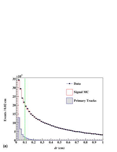
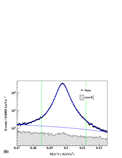
Figure 1: (color online) Selection of $K^{0}_{S}\to\pi^{+}\pi^{-}$ candidates in $\tau$ decays: (a) Distribution of the closest distance of approach to the IP in the $r-\phi$ plane for two $K^{0}_{S}$ daughter tracks of the $K^{0}_{S}$ candidates. The background represented by the shaded histogram, obtained by MC, consists of the tracks from primary vertex. (b) Distribution of the invariant mass $M(\pi^{+}\pi^{-})$ for the $K^{0}_{S}$ candidates after applying all selection requirements except the mass. The solid line is a fit with three Gaussians for the signal and a linear background. The shaded histogram stands for the background from $\tau^{-}\to\pi^{-}\pi^{+}\pi^{-}\nu_{\tau}$ obtained by MC. In both plots, the vertical lines represent the $K^{0}_{S}$ selection criteria.

III.2 Selection of events containing one $K^{0}_{S}$

For the modes with one $K^{0}_{S}$, the $K^{0}_{S}\to\pi^{+}\pi^{-}$ candidate is reconstructed from a pair of oppositely charged tracks. The $z$-distance between the two helices at the $\pi^{+}\pi^{-}$ vertex position ($z_{\rm dist}$) must be less than 2.5 cm. The pion momenta are then refitted with a common vertex constraint. The flight length ($\ell_{f}$) of the $K^{0}_{S}$ candidates must be between 2 cm and 20 cm. The distance of closest approach to the IP in the $r$–$\phi$ plane ($dr$) is required to be larger than 0.1 cm for each daughter in order to suppress the background from the tracks from the primary vertex. The $dr$ distribution is well reproduced by MC as shown in Fig. 1 (a). Figure 1 (b) shows the distribution of the $\pi^{+}\pi^{-}$ invariant mass of the $K^{0}_{S}$ candidates. A clear $K^{0}_{S}$ signal is seen with a small background that is less than 1%. The signal window is defined as the mass range 0.485 GeV/$c^{2}<M_{\pi\pi}<0.512$ GeV/$c^{2}$, which corresponds to a $\pm 5\sigma$ window.

Events containing at least one so-defined $K^{0}_{S}$ are assigned to the inclusive $K^{0}_{S}$ sample irrespective of the accompanying particles on the signal side. The number of inclusive $\tau^{-}\to K^{0}_{S}~{}X^{-}\nu_{\tau}$ events in this sample is obtained from a fit to the $\pi^{+}\pi^{-}$ invariant mass distribution that uses the sum of three Gaussians for the signal and a linear function for background. In the case where an event contains two or more $K^{0}_{S}$ candidates, one is chosen arbitrarily for the fit. The fit, shown as the solid curve in Fig. 1 (b), yields $397806\pm 631$ inclusive $K^{0}_{S}$ signal events.

For the modes with one $\pi^{0}$, $\pi^{-}K^{0}_{S}\pi^{0}\nu_{\tau}$ and $K^{-}K^{0}_{S}\pi^{0}\nu_{\tau}$, the $\pi^{0}$ candidate is reconstructed from the invariant mass of two photons detected on the signal side. The normalized mass difference between the invariant mass of the two photons and the nominal $\pi^{0}$ mass ($M_{\pi^{0}}$),

$$S_{\gamma\gamma}=(M_{\gamma\gamma}-M_{\pi^{0}})/\sigma_{\gamma\gamma},$$ (1)

(where $\sigma_{\gamma\gamma}$ is the resolution of the invariant mass of the two photons) is used to determine the number of genuine $\pi^{0}$’s and to estimate the level of background from sidebands. The value of $\sigma_{\gamma\gamma}$ ranges from 0.004 to 0.009 GeV/$c^{2}$, depending on the momentum and polar angle of the $\pi^{0}$ candidate. The $S_{\gamma\gamma}$ distribution for events with one charged track and one $K^{0}_{S}$ is shown in Fig. 2. The lower-side tail of the $S_{\gamma\gamma}$ distribution is primarily due to leakage of electromagnetic showers out of the CsI(Tl) crystals and the conversion of photons in the material located in front of the crystals. Good agreement between data and MC indicates that these effects are properly modeled by the MC simulation. We define the interval $-6<S_{\gamma\gamma}<5$ as the $\pi^{0}$ signal region. We also use both sideband regions, $8<|S_{\gamma\gamma}|<11$, for the estimation of the spurious $\pi^{0}$ background. The sideband subtraction effectively removes the contamination of the spurious $\pi^{0}$ background in the selected samples.

As an alternative method, we count the number of the $\pi^{0}$ signal events by fitting the $S_{\gamma\gamma}$ distribution with the following formula:

$$f(S_{\gamma\gamma})=N_{\pi^{0}}((1-\alpha)S_{1}(S_{\gamma\gamma})+\alpha S_{2}(S_{\gamma\gamma}))$$

$$+N_{\textrm{bg}}B(S_{\gamma\gamma}),$$ (2)

where $N_{\pi}^{0}$ and $N_{\textrm{bg}}$ are the yields of $\pi^{0}$ signal and non-$\pi^{0}$ background, respectively. $S_{1}(S_{\gamma\gamma})$ is the $\pi^{0}$ signal probability density function (PDF) where both photons from $\pi^{0}$ are detected by the ECL directly, while $S_{2}(S_{\gamma\gamma})$ is the $\pi^{0}$ signal PDF where at least one photon is converted by the material in front of the ECL. $B(S_{\gamma\gamma})$ is the PDF for non-$\pi^{0}$ background. The shapes of $S_{1}(S_{\gamma\gamma})$, $S_{2}(S_{\gamma\gamma})$ and $B(S_{\gamma\gamma})$ are obtained from the MC simulation and are parametrized with a logarithmic Gaussian for $S_{1}(S_{\gamma\gamma})$ and $S_{2}(S_{\gamma\gamma})$ and a linear function for $B(S_{\gamma\gamma})$. The functional form of the logarithmic Gaussian is given in Appendix. The parameter $\alpha$ is the probability that at least one $\gamma$ is converted. In the fit to the data, the value of $\alpha$ is fixed to the MC value. The fit results for the $S_{1}(S_{\gamma\gamma})$, $S_{2}(S_{\gamma\gamma})$, and $B(S_{\gamma\gamma})$ components are shown in Fig. 2. The area enclosed by the solid and dotted curves represents the signal $S_{1}(S_{\gamma\gamma})$ component, the area enclosed by the dotted and dot-dashed curves represents the $S_{2}(S_{\gamma\gamma})$ component, and the hatched area indicates the fake $\pi^{0}$ background. The $S_{2}(S_{\gamma\gamma})$ component has a tail in the lower $S_{\gamma\gamma}$ region, since part of the $\gamma$ energy is lost by the conversion. We obtain consistent results for the branching fraction for both methods and assign the difference, if any, as a systematic error.

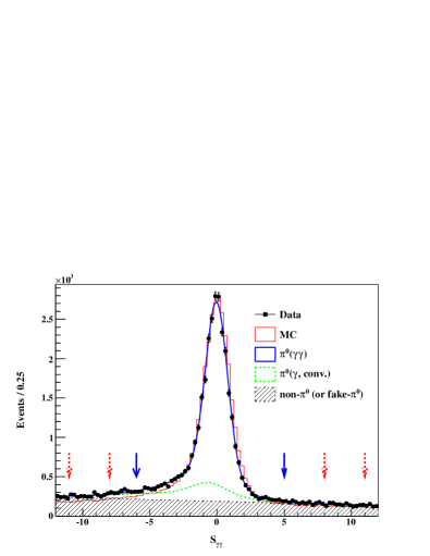
Figure 2: (color online) Distribution of the normalized two-photon invariant mass $S_{\gamma\gamma}=(M_{\gamma\gamma}-M_{\pi^{0}})/\sigma_{\gamma\gamma}$ for $\tau^{-}\to\pi^{-}K^{0}_{S}\pi^{0}\nu_{\tau}$ candidates. The arrows indicate the signal and sideband region. The area enclosed by the solid and dotted curves represents the true $\pi^{0}$ events reconstructed with two unconverted photons, the area enclosed by the dotted and the dot-dashed curves represents the true $\pi^{0}$ events reconstructed with at least one converted photon, while the hatched area indicates the fake $\pi^{0}$ background events.

The inclusive $K^{0}_{S}$ sample is further subdivided into exclusive modes according to the number of $K^{0}_{S}$ mesons, the number of charged hadrons and the number of $\pi^{0}$’s as: $\pi^{-}K^{0}_{S}\nu_{\tau}$, $K^{-}K^{0}_{S}\nu_{\tau}$, $\pi^{-}K^{0}_{S}\pi^{0}\nu_{\tau}$ and $K^{-}K^{0}_{S}\pi^{0}\nu_{\tau}$. In order to determine the exclusive decay mode and reduce the contribution from decay modes with multiple $\pi^{0}$’s, the sum of the energies of any photons that are located on the signal side and not used for the $\pi^{0}$ reconstruction is required to be smaller than 0.2 GeV for all modes. Finally, 157836 $\pi^{-}K^{0}_{S}\nu_{\tau}$, 32701 $K^{-}K^{0}_{S}\nu_{\tau}$, 26605 $\pi^{-}K^{0}_{S}\pi^{0}\nu_{\tau}$ and 8267 $K^{-}K^{0}_{S}\pi^{0}\nu_{\tau}$ candidates are selected.

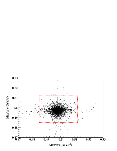
Figure 3: Two dimensional distribution of the $M(\pi^{+}\pi^{-})$ invariant masses for $K^{0}_{S}K^{0}_{S}$ candidate events in the $\tau$ decays. The dotted box is the $K^{0}_{S}K^{0}_{S}$ signal region.

The selected number of events, as well as the background and selection efficiency discussed below, are summarized in Table 1.

III.3 Selection of events containing two $K^{0}_{S}$ mesons

Since low branching fractions ($\mathcal{O}(10^{-4})$ – $\mathcal{O}(10^{-5})$) are expected for the modes with two $K^{0}_{S}$ mesons, several selection criteria are somewhat loosened for both $K^{0}_{S}$ candidates compared to those used to select single $K^{0}_{S}$ events in order to increase the signal efficiency. For the selection of $K^{0}_{S}$, the criteria for $dr$, $\ell_{f}$ and $z_{dist}$ are $dr>0.01\ \rm{cm}$, $\ell_{f}<50\ \rm{cm}$ and $z_{\rm dist}<3.5\ \rm{cm}$. In addition, the requirements for the tag side are loosened so that there is one charged track and any number of photons. No particle identification is required for the charged track.

Figure 3 shows the two-dimensional invariant mass of the $K^{0}_{S}K^{0}_{S}$ candidates; a clear $K^{0}_{S}K^{0}_{S}$ signal is seen with negligible background. The signal is selected within the signal box $0.485~{}\textrm{GeV}/c^{2}<M(\pi^{+}\pi^{-})<0.512~{}\textrm{GeV}/c^{2}$, corresponding to a $\pm 5\sigma$ window. The $\tau^{-}\rightarrow\pi^{-}K^{0}_{S}K^{0}_{S}(\pi^{0})\nu_{\tau}$ signal candidates are then selected with the condition of one $\pi^{-}$ and two $K^{0}_{S}$ (plus one $\pi^{0}$). Moreover, events where the energy sum of extra photons exceeds 0.3 GeV on the signal side are rejected. Finally, 6684 $\pi^{-}K^{0}_{S}K^{0}_{S}\nu_{\tau}$ and 303 $\pi^{-}K^{0}_{S}K^{0}_{S}\pi^{0}$ candidates are selected (summarized in Table 1).

III.4 Selection of two-lepton events

The two-lepton events where both $\tau$ leptons decay leptonically are used for the normalization of the branching fraction measurements. Only events with two leptons of different flavors (one electron and one muon) are used, since di-electron and di-muon events are contaminated by the radiative Bhabha and $e^{+}e^{-}\to\mu^{+}\mu^{-}(\gamma)$ processes, respectively. We require the opening angle between the two leptons to exceed $90^{\circ}$ in the CM. This procedure selects 7.66 $\times 10^{6}$ $e-\mu$ events.

A detailed study using simulated data indicates that the background comes from the two-photon process $e^{+}e^{-}\to e^{+}e^{-}\mu^{+}\mu^{-}(\gamma)$ (1.6%) and one-prong $\tau$ decay with leptonic $\tau$ decay on the other side, $\tau^{-}\to h^{-}(\pi^{0})\nu_{\tau}$, where $h^{-}=(\pi^{-}$, $K^{-})$ is misidentified as a lepton (2.6%). The total background fraction in selected events is found to be 4.2%. The detection efficiency is (19.31 $\pm$ 0.03)%. A comparison of the $e-\mu$ invariant mass distribution for data and MC, shown in Fig. 4, indicates good agreement and that the performance of the detector is well understood. In addition, the total number of $e-\mu$ events agrees within 0.38% with the expected number of events obtained from the integrated luminosity, the $\tau$-pair cross section, and the leptonic $\tau$ branching fractions. This result is consistent with the uncertainty estimated in the luminosity measurement.

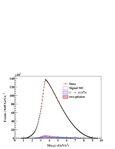
Figure 4: (color online) Distribution of $e-\mu$ invariant mass. The closed circles are data and the histogram is the sum of the signal and background in the MC. The hatched region and cross-hatched regions are the contributions from $\tau^{-}\to\pi^{-}\pi^{0}\nu_{\tau}$ and two-photon processes, respectively.

Table 1: Results of the event selection. Total efficiency ($\epsilon$), number of selected events ($N^{\rm Data}$), background fraction ($R^{\rm Bg}=N^{\rm Bg}/N^{\rm Data}$), and number of signal events after background subtraction and efficiency correction ($N^{\rm Sig}$). The $\epsilon$ includes the $K^{0}_{S}\to\pi^{+}\pi^{-}$ branching fraction.

Decay mode	$\epsilon$ (%)	$N^{\rm Data}$	$R^{\rm Bg}(\%)$	$N^{\rm Sig}$
$K^{0}_{S}~{}X^{-}$	9.66	$397806\pm 631$	$4.20\pm 0.46$	$(3.947\pm 0.007)\times 10^{6}$
$\pi^{-}K^{0}_{S}$	7.09	$157836\pm 541$	$8.86\pm 0.05$	$(1.793\pm 0.005)\times 10^{6}$
$K^{-}K^{0}_{S}$	6.69	$32701\pm 295$	$3.55\pm 0.07$	$(3.193\pm 0.018)\times 10^{5}$
$\pi^{-}K^{0}_{S}\pi^{0}$	2.65	$26605\pm 208$	$5.60\pm 0.10$	$(8.336\pm 0.070)\times 10^{5}$
$K^{-}K^{0}_{S}\pi^{0}$	2.19	$8267\pm 109$	$2.43\pm 0.10$	$(3.226\pm 0.045)\times 10^{5}$
$\pi^{-}K^{0}_{S}K^{0}_{S}$	2.47	$6684\pm 96$	$7.89\pm 0.24$	$(2.447\pm 0.033)\times 10^{5}$
$\pi^{-}K^{0}_{S}K^{0}_{S}\pi^{0}$	0.82	$303\pm 33$	$11.60\pm 1.60$	$(2.105\pm 0.140)\times 10^{4}$

IV Determination of the branching fractions

IV.1 Formula for branching fraction measurements

We use two different normalization methods for the determination of the branching fractions: one uses the number of $e-\mu$ events while the other uses the integrated luminosity. As the number of $e-\mu$ events obtained from $\tau$-pair selection is consistent with the one deduced from the integrated luminosity measurement within 0.38%, the normalization using either of them will lead to consistent results. However, the resulting systematic uncertainties for the branching fraction measurements differ.

In the first method, the branching fraction is given by the formula

$$\mathcal{B}_{i}=\frac{N^{\rm Sig}_{i}}{N^{\rm Sig}_{e\textrm{-}\mu}}\frac{\mathcal{B}_{e}\mathcal{B}_{\mu}}{\mathcal{B}_{e}+\mathcal{B}_{\mu}},$$ (3)

where $i$ represents the decay mode under study and $N^{\rm Sig}_{i}$ is the number of signal events after efficiency and background corrections, where one $\tau$ lepton decays into a signal mode and the other $\tau$ decays leptonically. $N^{\rm Sig}_{e\textrm{-}\mu}$ is the number of $e-\mu$ events after efficiency and background corrections. $\mathcal{B}_{e}$ and $\mathcal{B}_{\mu}$ are the branching fractions for $\tau^{-}\to e^{-}\bar{\nu}_{e}\nu_{\tau}$ and $\tau^{-}\to\mu^{-}\bar{\nu}_{\mu}\nu_{\tau}$, respectively. The world-average values, $\mathcal{B}_{e}=(17.83\pm 0.04)\%$ and $\mathcal{B}_{\mu}=(17.41\pm 0.04)\%$ Beringer et al. (2012), are used. In this formula, the systematics coming from the luminosity measurement, tracking efficiency and the particle identification efficiency cancel (completely or partially) in the ratio. The branching fractions for the inclusive $\tau^{-}\to K^{0}_{S}X^{-}\nu_{\tau}$ and four exclusive decay modes, $\tau^{-}\to\pi^{-}K^{0}_{S}\nu_{\tau}$, $K^{-}K^{0}_{S}\nu_{\tau}$, $\pi^{-}K^{0}_{S}\pi^{0}\nu_{\tau}$, $K^{-}K^{0}_{S}\pi^{0}\nu_{\tau}$, are obtained using this formula.

Statistical uncertainty is an important issue for the modes with two $K^{0}_{S}$’s: $\tau^{-}\rightarrow\pi^{-}K^{0}_{S}K^{0}_{S}\nu_{\tau}$ and $\tau^{-}\rightarrow\pi^{-}K^{0}_{S}K^{0}_{S}\pi^{0}\nu_{\tau}$. For these modes, we use all one-prong decay modes on the tag side and determine the branching fraction using the luminosity measured using the Bhabha process:

$$\mathcal{B}_{i}=\frac{N^{\rm Sig}_{i}}{2N_{\tau\bar{\tau}}\mathcal{B}_{1-\rm prong}},$$ (4)

where $\mathcal{B}_{1-\rm prong}$ is the one-prong decay branching fraction of $(85.35\pm 0.07)\%$. $N_{\tau\tau}=\mathcal{L}\sigma_{\tau\tau}$ is the number of produced $\tau$ pairs determined from the luminosity, $\mathcal{L}=(669\pm 9){\rm fb}^{-1}$, and the $\tau$-pair production cross section $\sigma_{\tau\tau}=(0.919\pm 0.003){\rm nb}$ Banerjee et al. (2008). $N^{\rm Sig}_{i}$ is the number of signal events after efficiency and background corrections.

In both cases, the number of signal events is determined simultaneously by using the inverse efficiency matrix to take into account the cross-feed from one decay mode into another:

$$N^{\rm Sig}_{i}=\sum_{j}(\mathcal{E}^{-1})_{ij}(N^{\rm Data}_{j}-N^{\rm Bg}_{j}),$$ (5)

where $i$ represents the true decay mode of interest and $j$ represents the reconstructed decay mode. $N^{\rm Data}_{j}$ is the number of selected events in the $j$-th decay mode and $N^{\rm Bg}_{j}$ is the background coming from decay modes other than the six modes under consideration together with the non-$\tau$ processes. Hereinafter, we use “background” to mean this. $\mathcal{E}^{-1}$ is the inverse of the selection efficiency matrix ($\mathcal{E}_{ji}$ being the probability of reconstructing a true decay type $i$ as a decay type $j$).

IV.2 Background and efficiency

IV.2.1 Background

The number of background events from $\tau$ decays other than the six modes analyzed here is determined by the TAUOLA MC using the world-average (PDG) branching fractions Beringer et al. (2012). The uncertainties of the PDG branching fractions are used as a measure of the background uncertainty.

The non-$\tau$ decay contributions are dominated by $q\bar{q}$ continuum events. The background from $q\bar{q}$ for each mode is confirmed with the data and MC simulation control sample. The control sample is prepared with the same selection criteria as the signal, but requiring that the invariant mass of the hadron system be larger than the $\tau$ mass. With this selection, one eliminates the $\tau$-pair events and enhances the number of $q\bar{q}$ events. The number of selected events in data and MC are found to be consistent within 20%. From this calibration, the $q\bar{q}$ background is found to be 0.2–0.8% for the one-$K^{0}_{S}$ categories. On the other hand, the two-$K^{0}_{S}$ categories have large $q\bar{q}$ background: the fraction is 8–12%. The difference between data and MC in the control region is taken as a systematic error of the $q\bar{q}$ background estimation. Backgrounds from $B\bar{B}$ and two-photon processes are negligible: 0.1–0.5% for two-photon events and $<$ 0.1% for $B\bar{B}$. The fraction of the total background for each mode, summarized in the fourth column of Table 1, ranges from 2.4% to 12%.

IV.2.2 Calibration and corrections

The particle identification efficiencies, as well as the $K^{0}_{S}$ and $\pi^{0}$ reconstruction efficiencies, are critical issues for this analysis and difficult to reproduce using MC with the required precision; it is necessary to calibrate them using data. For this purpose, several control samples are prepared for data and MC in order to check the reliability of the MC simulation, and correction tables are constructed.

The calibration of the particle identification efficiency for charged pions and kaons is carried out using kinematically identified $D^{*-}\to D^{0}\pi^{-}$($D^{0}\to K^{-}\pi^{+}$) decays, where the kaon and pion from the $D^{0}$ decay are known from the charge of the accompanying slow pion. We evaluate the identification efficiencies and misidentification probabilities for this calibration sample and compare them to MC expectations. From this comparison, we obtain correction factors as a function of track momentum and polar angle and apply these to the MC. The average correction factor for pions (kaons) is $0.971\pm 0.007$ ($1.002\pm 0.001$). The accuracy of the correction factor, which is a source of the systematic uncertainty for the evaluation of the branching fraction, is limited by the statistical uncertainties of the kaon and pion sample from $D^{*-}$ decays in certain momentum and angular bins and the uncertainty of the $D^{*-}$ signal extraction.

The calibration of the efficiency for electrons and muons is carried out using two-photon events from the reaction $e^{+}e^{-}\to e^{+}e^{-}\ell^{+}\ell^{-}$($\ell=e,\mu$). The efficiency correction table constructed for the two-dimensional space of momentum and polar angle in the laboratory frame and then applied to the Monte Carlo efficiencies. In this way, the uncertainty on the lepton efficiency is determined by the statistics of the two-photon data sample and its long-term stability. The latter is evaluated from the variation of the corrections calculated using time-ordered subsets of the experimental two-photon data. The average corrections are $0.981\pm 0.008$ for electrons and $0.958\pm 0.005$ for muons.

The reconstruction efficiency for the $K^{0}_{S}$ as a function of momentum has been studied by using a control sample from the decay chain $D^{*-}\rightarrow D^{0}\pi^{-},D^{0}\rightarrow K^{0}_{S}\pi^{+}\pi^{-}$. The number of $K^{0}_{S}$ signal events that satisfy the full selection is compared with the value determined by only fitting the invariant mass distribution without any requirements on the secondary vertex reconstruction. The average correction factor is 0.979 $\pm$ 0.007.

The $\pi^{0}$ reconstruction efficiency is studied using a sample in which both $\tau$ leptons decay into $h^{\pm}\pi^{0}\nu_{\tau}$, where $h^{\pm}$ stands for $\pi^{\pm}$ or $K^{\pm}$. In the study, we first measure the ratio

$$R_{i}=N(h^{-}\pi^{0}\nu_{\tau}|h^{+}\pi^{0}\bar{\nu}_{\tau})/N(h^{-}\pi^{0}\nu_{\tau}|\ell^{+}\nu_{\ell}\bar{\nu}_{\tau})$$ (6)

for experimental data and the MC ($i$=data, MC). Here, $N(h^{-}\pi^{0}\nu_{\tau}|h^{+}\pi^{0}\bar{\nu}_{\tau})$ is the number of events with both $\tau$ leptons decaying to $h^{\pm}\pi^{0}\nu_{\tau}$ ($double~{}h\pi^{0}$), while $N(h^{-}\pi^{0}\nu_{\tau}|\ell^{+}\nu_{\ell}\bar{\nu}_{\tau})$ is the number of events where one $\tau$ decays to $h^{-}\pi^{0}\nu_{\tau}$ and the other to $\ell^{+}\bar{\nu_{\ell}}\nu_{\tau}$ ($single~{}h\pi^{0}$). We then take the double ratio $R=R_{\rm data}/R_{\rm MC}$ in which many common factors, such as the normalization and tracking efficiency, cancel. If we rely on the world-average branching fractions for $\tau^{-}\to h^{-}\pi^{0}\nu_{\tau}$ and $\tau^{-}\to\ell^{-}\bar{\nu}_{\ell}\nu_{\tau}$, the double ratio depends on the product of the corrections of the $\pi^{0}$ reconstruction and lepton ID efficiencies only, where the latter is well-known from the two-photon events as well as other studies. From the double ratio $R$, the MC-data correction for the $\pi^{0}$ efficiency is determined to be $R=0.957\pm 0.015$. A result consistent with this value is also obtained from a study using $\eta$ decays, where the ratio of the number of $\eta$ events reconstructed from $\eta\to\gamma\gamma$ and $\eta\to 3\pi^{0}$ is compared in experimental data and MC.

Table 2: Probabilities $\mathcal{E}_{ji}$ of the efficiency matrix for reconstructing a true decay type $i$ as a decay type $j$, in %, for the six decay modes under study. The first four rows shows the efficiency matrix for lepton tagging, while the last two rows show efficiencies for lepton and hadron tagging. The efficiencies include the $K^{0}_{S}\to\pi^{+}\pi^{-}$ branching fraction. The dash indicates values smaller than 0.01%.

Selected	True Decay mode
decay mode	$\pi^{-}K^{0}_{S}$	$K^{-}K^{0}_{S}$	$\pi^{-}K^{0}_{S}\pi^{0}$	$K^{-}K^{0}_{S}\pi^{0}$	$\pi^{-}K^{0}_{S}K^{0}_{S}$	$\pi^{-}K^{0}_{S}K^{0}_{S}\pi^{0}$
$\pi^{-}K^{0}_{S}$	7.09	1.65	1.07	0.31	0.67	0.13
$K^{-}K^{0}_{S}$	0.35	6.69	0.06	1.01	0.04	0.01
$\pi^{-}K^{0}_{S}\pi^{0}$	—	—	2.65	0.54	0.51	0.23
$K^{-}K^{0}_{S}\pi^{0}$	—	—	0.11	2.19	0.01	—
$\pi^{-}K^{0}_{S}K^{0}_{S}$	—	—	—	—	2.47	0.53
$\pi^{-}K^{0}_{S}K^{0}_{S}\pi^{0}$	—	—	—	—	0.04	0.81

Table 3: Uncertainties $[\sigma_{\mathcal{E}}]_{ji}$ on the efficiency matrix (in %). The dash indicates values smaller than 0.001%.

Selected	True Decay mode
decay mode	$\pi^{-}K^{0}_{S}$	$K^{-}K^{0}_{S}$	$\pi^{-}K^{0}_{S}\pi^{0}$	$K^{-}K^{0}_{S}\pi^{0}$	$\pi^{-}K^{0}_{S}K^{0}_{S}$	$\pi^{-}K^{0}_{S}K^{0}_{S}\pi^{0}$
$\pi^{-}K^{0}_{S}$	0.119	0.069	0.018	0.013	0.011	0.002
$K^{-}K^{0}_{S}$	0.011	0.116	0.002	0.018	0.001	—
$\pi^{-}K^{0}_{S}\pi^{0}$	—	—	0.060	0.025	0.009	0.005
$K^{-}K^{0}_{S}\pi^{0}$	—	—	0.004	0.050	—	—
$\pi^{-}K^{0}_{S}K^{0}_{S}$	—	—	—	—	0.071	0.015
$\pi^{-}K^{0}_{S}K^{0}_{S}\pi^{0}$	—	—	—	—	0.001	0.027

IV.2.3 Efficiency matrix

After taking into account the corrections discussed in the previous subsection, the efficiency matrix $\mathcal{E}_{ji}$ is obtained. The values of $\mathcal{E}_{ji}$ and their uncertainties are summarized in Tables 2 and 3, respectively. For example, the efficiency for selecting a true $\tau^{-}\rightarrow\pi^{-}K^{0}_{S}\nu_{\tau}$ decay as a $\pi^{-}K^{0}_{S}$ or $K^{-}K^{0}_{S}$ candidates is $(7.09\pm 0.12)\%$ and $(0.35\pm 0.01)\%$, respectively. The uncertainty of the first efficiency is dominated by the uncertainty of the pion and lepton identification efficiency (0.8%) and the $K^{0}_{S}$ reconstruction efficiency (1.4%), while the uncertainty of the second efficiency is dominated by uncertainty of the misidentification efficiency from pion to kaon (3%). (The detailed discussions of these uncertainties are given in the next subsections.)

The efficiency for selecting a true $\tau^{-}\rightarrow\pi^{-}K^{0}_{S}\pi^{0}\nu_{\tau}$ decay as a $\pi^{-}K^{0}_{S}\pi^{0}$ or $\pi^{-}K^{0}_{S}$ candidate is $(2.65\pm 0.06)\%$ and $(1.07\pm 0.02)\%$, respectively. The uncertainty of the first efficiency includes the uncertainties for the charged pion, $K^{0}_{S}$ and $\pi^{0}$ identification. The uncertainty of the $\pi^{0}$ identification is estimated to be 1.5%. The same uncertainty is assigned to the decays without the $\pi^{0}$ meson.

It is worth noting that the migration efficiency for the modes without $\pi^{0}$ selected as the modes with $\pi^{0}$ is negligible because, as mentioned, the spurious $\pi^{0}$ mesons are subtracted using the events in the $\pi^{0}$ sideband region.

IV.3 Systematic uncertainties

The sources of systematic uncertainties can be categorized as those related to detection/reconstruction efficiencies and other items such as hadron decay models, background estimation, normalization and event selection such as the $\gamma$ veto. The efficiencies have several uncertainties, arising from track finding, particle identification, $K^{0}_{S}$ and $\pi^{0}$ reconstruction and the $\pi^{0}$ sideband subtraction.

IV.3.1 Uncertainty of tracking and particle identification

The uncertainty of the charged track finding efficiency is 0.35% per charged track. Since the track finding uncertainty partially cancels in Eq. (3), the net uncertainty is 0.7% for the modes with one $K^{0}_{S}$ and 2.1% for the modes with two $K^{0}_{S}$, where the uncertainty for tracking efficiency is added linearly assuming 100% correlation.

The uncertainties due to particle identification are estimated from the precision of the efficiency calibration procedure. The uncertainty for the pion and kaon efficiency is found to be 0.4% and 0.8%, respectively. The uncertainties for misidentification from pion to kaon and vice versa are found to be 3% for each. The uncertainty for electron (muon) identification is 0.8% (0.5%).

The efficiency for the $K^{0}_{S}$ reconstruction is studied using a $K^{0}_{S}$ control sample from the $D^{*}\rightarrow\pi_{s}D^{0}$, $D^{0}\rightarrow K^{0}_{S}\pi^{+}\pi^{-}$ decay chain by comparing the $K^{0}_{S}$ yields with and without vertex reconstruction (0.7%) as well as by varying the requirements on $dr$, $z_{dist}$, $\ell_{f}$, and the $M(\pi^{+}\pi^{-})$ window (1.2%). The net uncertainty from $K^{0}_{S}$ reconstruction is estimated to be 1.4%.

IV.3.2 Uncertainty of $\pi^{0}$ reconstruction

The uncertainty due to the correction of the $\pi^{0}$ efficiency is determined by using $\tau^{-}\to h^{-}\pi^{0}\nu_{\tau}$ samples. The dominant uncertainty for $\pi^{0}$ efficiency comes from the method of counting the number of $\pi^{0}$ events. Two methods, one using the subtraction of sideband events and the other using fits with a logarithmic Gaussian, are used to estimate the signal and background $\pi^{0}$. The uncertainty of the $\pi^{0}$ efficiency is estimated to be 1.5%.

Table 4: Summary of the relative statistical and systematic uncertainties. The values in the row “Efficiency matrix” show the diagonal elements of the covariant matrix in the first term of Eq. (7), which correspond to the total uncertainties of the tracking, particle identification, and $\pi^{0}$ and $K^{0}_{S}$ reconstruction efficiencies. Each contribution is shown as sub-items using parentheses. The total systematic uncertainty is obtained from the diagonal element of the covariance matrix given in Eq. (7).

	$\bigtriangleup\mathcal{B}/\mathcal{B}$ (%)
Error Source	$K^{0}_{S}~{}X^{-}$	$\pi^{-}K^{0}_{S}$	$K^{-}K^{0}_{S}$	$\pi^{-}K^{0}_{S}\pi^{0}$	$K^{-}K^{0}_{S}\pi^{0}$	$\pi^{-}K^{0}_{S}K^{0}_{S}$	$\pi^{-}K^{0}_{S}K^{0}_{S}\pi^{0}$
Statistical uncertainty	0.2	0.3	0.9	0.8	1.3	1.4	10.8
Efficiency matrix	1.6	1.7	2.1	2.3	2.4	2.9	4.0
Track finding	(0.7)	(0.7)	(0.8)	(0.7)	(0.7)	(2.1)	(2.7)
Particle ID	(—)	(0.6)	(1.0)	(0.7)	(0.8)	(0.8)	(1.0)
$K^{0}_{S}$ reconstruction	(1.4)	(1.4)	(1.5)	(1.4)	(1.4)	(1.8)	(2.3)
$\pi^{0}$ reconstruction	(—)	(0.1)	(0.2)	(1.5)	(1.5)	(0.0)	(1.5)
Hadron decay model	—	—	0.7	0.3	3.4	1.2	4.2
Background	0.5	0.2	0.3	1.9	0.4	1.8	3.2
Normalization	0.5	0.5	0.5	0.5	0.5	1.4	1.4
$\gamma$ veto	—	0.1	1.8	1.2	1.5	1.0	2.0
Total systematic uncertainty	1.7	1.8	3.7	3.5	4.9	4.0	10.1

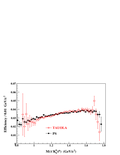
Figure 5: (color online) Efficiency as a function of the hadron mass for $\tau^{-}\rightarrow\pi^{-}K^{0}_{S}\pi^{0}\nu_{\tau}$. The open circles are the efficiencies obtained using the TAUOLA event generator. The closed circles are obtained assuming a uniform angular decay distributions. The tagging and branching fraction factors are included in the value of the efficiency.

IV.3.3 Decay model dependence of the efficiency

The signal efficiency can potentially change depending on the dynamics of the hadronic system. A test is performed with a set of MC events generated according to phase space (PS) in addition to the standard MC sample based on TAUOLA. For both sets, the invariant mass distribution for the full hadronic system has been tuned to agree with that of experimental data. The subsystem mass distribution in the three- or four-body decays and their angular distributions differ between the TAUOLA and PS models. The efficiency as a function of the $\pi^{-}K^{0}_{S}\pi^{0}$ invariant mass in $\tau^{-}\to\pi^{-}K^{0}_{S}\pi^{0}\nu_{\tau}$ is shown in Fig. 5 for these models. In both cases, the efficiency changes smoothly as a function of hadronic mass and the efficiencies at the same hadronic mass agree in both cases except for the mass region above 1.7 GeV/$c^{2}$. This agreement indicates that the efficiency is insensitive to the detailed decay models of the hadronic system. We obtain the net efficiency for the full mass region in both models and assign the difference between them as a systematic uncertainty due to the decay model. The resultant model dependences for $\pi K^{0}_{S}\nu_{\tau}$, $K^{-}K^{0}_{S}\nu_{\tau}$, $K^{-}K^{0}_{S}\pi^{0}\nu_{\tau}$, $\pi^{-}K^{0}_{S}K^{0}_{S}\nu_{\tau}$ and $\pi^{-}K^{0}_{S}K^{0}_{S}\pi^{0}\nu_{\tau}$, range from 0.3 to 4.2% as shown in the row labeled “Hadron decay model” in Table 4.

IV.3.4 Uncertainty of the background

The uncertainty due to the background from other $\tau$ decays is estimated from the uncertainties of the world-average branching fractions given in the PDG listing Beringer et al. (2012). The uncertainty of the continuum background is estimated from the difference between MC and data for the control sample above the $\tau$ mass. Adding the uncertainty from other $\tau$ decays and the uncertainty of the $q\bar{q}$ continuum in quadrature, the background uncertainties for each decay mode are in the range from 0.2% to 3.2% as shown in Table 4.

IV.3.5 Uncertainty of the normalization

The uncertainty due to the normalization is 0.5% for the modes that use $e-\mu$ events for the normalization, while the uncertainty for $\pi^{-}K^{0}_{S}K^{0}_{S}\nu_{\tau}$ and $\pi^{-}K^{0}_{S}K^{0}_{S}\pi^{0}\nu_{\tau}$ is 1.4%. The former uncertainty includes the uncertainty of $\mathcal{B}(\tau^{-}\rightarrow l^{-}\nu_{l}\nu_{\tau})$ ($0.1\%$) and the background uncertainty in $e-\mu$ event selection (less than $0.1\%$). The latter is dominated by the uncertainty of the luminosity measurement.

IV.3.6 Uncertainty of the $\gamma$ veto

The uncertainty due to the $\gamma$ veto is obtained by varying the condition on the energy sum of extra photons $E^{\rm ex}_{\gamma}$ from 0.2 GeV to 1.0 GeV. The uncertainties for each mode range from 0.1% to 2.0% as shown in Table 4.

Table 5: Correlation coefficients between the branching fraction measurements. Both statistical and systematic errors are included.

	$\pi^{-}K^{0}_{S}$	$K^{-}K^{0}_{S}$	$\pi^{-}K^{0}_{S}\pi^{0}$	$K^{-}K^{0}_{S}\pi^{0}$	$\pi^{-}K^{0}_{S}K^{0}_{S}$	$\pi^{-}K^{0}_{S}K^{0}_{S}\pi^{0}$
$\pi^{-}K^{0}_{S}$	1	-0.230	-0.132	0.023	-0.019	0.004
$K^{-}K^{0}_{S}$		1	0.043	-0.215	-0.001	0.000
$\pi^{-}K^{0}_{S}\pi^{0}$			1	-0.204	-0.063	0.006
$K^{-}K^{0}_{S}\pi^{0}$				1	0.002	0.000
$\pi^{-}K^{0}_{S}K^{0}_{S}$					1	-0.230
$\pi^{-}K^{0}_{S}K^{0}_{S}\pi^{0}$						1

IV.3.7 Covariance matrix and error propagation

Taking into account all uncertainties discussed in the previous sections, we obtain the covariance matrix for the measured branching fractions. Since the branching fractions are determined simultaneously by solving linear equations, there is a correlation among the results. These correlations are taken into account by the covariance matrix. The full covariance matrix cov($\mathcal{B}_{i},\mathcal{B}_{j}$) is given by the formula provided in Ref. Lefebvre et al. (2000),

$${\rm cov}(\mathcal{B}_{i},\mathcal{B}_{j})=f_{a}f_{b}{\rm cov}(\mathcal{E}^{-1}_{ia},\mathcal{E}^{-1}_{jb})+\mathcal{E}^{-1}_{ik}\mathcal{E}^{-1}_{jl}{\rm cov}(f_{k},f_{l}),$$ (7)

where the indices indicate the decay modes of interest, and the summation is assumed implicitly if the same index is repeated. The quantity $f_{j}$ is defined by $\mathcal{B}_{i}=\sum_{j}\mathcal{E}^{-1}_{ij}f_{j}$ and is given by

$$f_{j}=\frac{(N^{\rm Data}_{j}-N^{\rm Bg}_{j})}{N^{\rm Sig}_{e\textrm{-}\mu}}\frac{\mathcal{B}_{e}\mathcal{B}_{\mu}}{\mathcal{B}_{e}+\mathcal{B}_{\mu}}$$ (8)

and

$$f_{j}=\frac{(N^{\rm Data}_{j}-N^{\rm Bg}_{j})}{2N_{\tau\bar{\tau}}\mathcal{B}_{1-\rm prong}}$$ (9)

for the one $K^{0}_{S}$ and $K^{0}_{S}K^{0}_{S}$ cases, respectively.

The first term in Eq. (7) represents the covariance due to the inverse of the efficiency matrix $\mathcal{E}_{ji}$. Assuming that the elements $\mathcal{E}_{ji}$ are uncorrelated, the term ${\rm cov}(\mathcal{E}^{-1}_{\alpha\beta},\mathcal{E}^{-1}_{ab})$ can be expressed as

$${\rm cov}(\mathcal{E}^{-1}_{\alpha\beta},\mathcal{E}^{-1}_{ab})=(\mathcal{E}^{-1}_{\alpha j}\mathcal{E}^{-1}_{aj})[\sigma_{\mathcal{E}}]^{2}_{ji}(\mathcal{E}^{-1}_{i\beta}\mathcal{E}^{-1}_{ib}).$$ (10)

where $[\sigma_{\mathcal{E}}]_{ji}$ is the error of ${\mathcal{E}}_{ji}$. The values of $[\sigma_{\mathcal{E}}]_{ji}$ are summarized in Table 3. The error includes the uncertainties due to the track finding, particle identification, $\pi^{0}$ and $K^{0}_{S}$ reconstruction efficiencies.

Using Eq. (10), the correlations of the uncertainty for the track finding, particle identification and $K^{0}_{S}$ and $\pi^{0}$ reconstruction efficiencies for the individual modes as well as the cross-feed among the modes are taken into account. The total uncertainty as well as each contribution are summarized in the row of “Efficiency matrix” and its sub-items in Table 4.

The second term in Eq. (7) includes the uncertainties from the quantities contained in Eq. (8) and Eq. (9), such as the common normalization, the background, and the statistical uncertainty. We also include the model dependence and the $\gamma$ veto in this term.

Adding all systematic errors in Eq. (7), the total covariance matrix ${\rm cov}(\mathcal{B}_{i},\mathcal{B}_{j})$ of the systematic uncertainty is obtained. The square root of the diagonal element, $\sqrt{{\rm cov}(\mathcal{B}_{i},\mathcal{B}_{i})}$, is given in the last row of Table 4. The correlation coefficients, defined as ${\rm cov}(\mathcal{B}_{i},\mathcal{B}_{j})/\sqrt{{\rm cov}(\mathcal{B}_{i},\mathcal{B}_{i})~{}{\rm cov}(\mathcal{B}_{j},\mathcal{B}_{j})}$, are presented in Table 5, where both systematic and statistical uncertainties are included. The largest correlation of about $-0.23$ is observed for the modes where a charged pion and kaon are interchanged.

Table 6: Summary of the branching fractions of the $\tau$ lepton decays to one or more $K^{0}_{S}$ obtained in this experiment and previous experiments. The first uncertainty is statistical and the second is systematic.

Mode	Branching Fraction	Ref.
$K^{0}_{S}~{}X^{-}\nu_{\tau}$	$(9.15\pm 0.01\pm 0.15)\times 10^{-3}$	This exp.
$\pi^{-}K^{0}_{S}\nu_{\tau}$	$(4.16\pm 0.01\pm 0.08)\times 10^{-3}$	This exp.
$K^{-}K^{0}_{S}\nu_{\tau}$	$(7.40\pm 0.07\pm 0.27)\times 10^{-4}$	This exp.
$\pi^{-}K^{0}_{S}\pi^{0}\nu_{\tau}$	$(1.93\pm 0.02\pm 0.07)\times 10^{-3}$	This exp.
$K^{-}K^{0}_{S}\pi^{0}\nu_{\tau}$	$(7.48\pm 0.10\pm 0.37)\times 10^{-4}$	This exp.
$\pi^{-}K^{0}_{S}K^{0}_{S}\nu_{\tau}$	$(2.33\pm 0.03\pm 0.09)\times 10^{-4}$	This exp.
$\pi^{-}K^{0}_{S}K^{0}_{S}\pi^{0}\nu_{\tau}$	$(2.00\pm 0.22\pm 0.20)\times 10^{-5}$	This exp.
$\pi^{-}K^{0}_{S}K^{0}_{L}\nu_{\tau}$	$(1.01\pm 0.23\pm 0.13)\times 10^{-3}$	ALEPH Barate et al. (1998)
$\pi^{-}K^{0}_{S}\pi^{0}\pi^{0}\nu_{\tau}$	$(0.13\pm 0.12\pm 0.00)\times 10^{-3}$	ALEPH Barate et al. (1999b)
$\pi^{-}K^{0}_{S}\eta\nu_{\tau}$	$(0.44\pm 0.07\pm 0.03)\times 10^{-3}$	Belle Inami et al. (2009)
$\pi^{-}K^{0}_{S}K^{0}_{L}\pi^{0}\nu_{\tau}$	$(0.31\pm 0.11\pm 0.05)\times 10^{-3}$	ALEPH Barate et al. (1999b)
$K^{0}_{S}h^{-}h^{+}h^{-}\nu_{\tau}$	$(0.115\pm 0.095\pm 0.04)\times 10^{-3}$	ALEPH Barate et al. (1998)

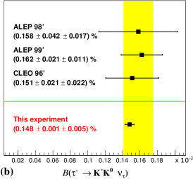
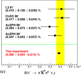
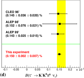
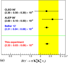
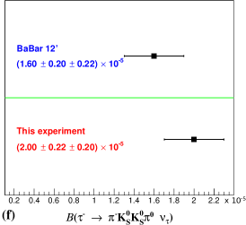
Figure 6: (color online) Comparison of results on the branching fractions from this work and previous measurements for the six decay modes : (a) $\pi^{-}\bar{K}^{0}\nu_{\tau}$, (b) $K^{-}K^{0}\nu_{\tau}$, (c) $\pi^{-}\bar{K}^{0}\pi^{0}\nu_{\tau}$, (d) $K^{-}K^{0}\pi^{0}\nu_{\tau}$, (e) $\pi^{-}K^{0}_{S}K^{0}_{S}\nu_{\tau}$ and (f) $\pi^{-}K^{0}_{S}K^{0}_{S}\pi^{0}\nu_{\tau}$. The band represents the pre-$B$-factory world averages and their uncertainties Beringer et al. (2012).

IV.4 Branching fractions and discussion

IV.4.1 Inclusive branching fraction

The branching fraction for inclusive $K^{0}_{S}$, $\mathcal{B}(\tau^{-}\to K_{S}^{0}X^{-}\nu_{\tau})$, is determined from the total size of the inclusive $K^{0}_{S}$ sample discussed in Section III.2 using Eq. (3). By applying the corrections for the PID and $K^{0}_{S}$ reconstruction, the signal efficiency is $(9.66\pm 0.15)\%$ while the background admixture is $(4.20\pm 0.17)\%$ among the total selected events. The background is dominated by the $q\bar{q}$ continuum. The systematic uncertainty is estimated to be 1.7%. The resulting branching fraction is

$$\mathcal{B}(\tau^{-}\rightarrow K^{0}_{S}X^{-}\nu_{\tau})=(9.15\pm 0.01\pm 0.15)\times 10^{-3}.$$

IV.4.2 Exclusive branching fractions

The branching fractions of the six exclusive modes, $\pi^{-}K^{0}_{S}\nu_{\tau}$, $K^{-}K^{0}_{S}\nu_{\tau}$, $\pi^{-}K^{0}_{S}\pi^{0}\nu_{\tau}$, $K^{-}K^{0}_{S}\pi^{0}\nu_{\tau}$, $\pi^{-}K^{0}_{S}K^{0}_{S}\nu_{\tau}$ and $\pi^{-}K^{0}_{S}K^{0}_{S}\pi^{0}\nu_{\tau}$, are summarized in Table 6. The precision ranges from 1.8% to 7.5% and the systematic uncertainty is dominant except for the mode $\tau^{-}\to\pi^{-}K^{0}_{S}K^{0}_{S}\pi^{0}\nu_{\tau}$.

Figure 6 compares the branching fractions obtained in this and previous experiments. Assuming that $K^{0}-\bar{K}^{0}$ mixing is negligible, the branching fractions involving $K^{0}$ are twice those with $K^{0}_{S}$. The accuracy of the branching fractions is improved by a factor of five to ten compared to the pre-$B$-factory experiments. The branching fraction for $\tau^{-}\rightarrow\pi^{-}K^{0}_{S}\nu_{\tau}$ is consistent with our previous result Epifanov et al. (2007) with improved precision and supersedes our previous result. Our result also agrees with BaBar ($\mathcal{B}(\tau^{-}\to\pi^{-}\bar{K}^{0}\nu_{\tau})=(8.40\pm 0.03\pm 0.23)\times 10^{-3}$ Aubert et al. (2009)) within uncertainties. Recently, the branching fraction for $\tau^{-}\to\pi^{-}\bar{K}^{0}\nu_{\tau}$ has been estimated using the crossed channel branching fraction $\mathcal{B}(K\to\pi e\bar{\nu}_{e})$ and the measured $K_{S}^{0}\pi^{-}$ mass spectrum Antonelli et al. (2013). The result is $\mathcal{B}(\tau^{-}\to\pi^{-}\bar{K}^{0}\nu_{\tau})_{\rm Kaon}=(8.57\pm 0.30)\times 10^{-3}$. Our result is consistent with this prediction within uncertainties.

The branching fractions for $\tau^{-}\to K^{-}K^{0}_{S}\nu_{\tau}$ and $\tau^{-}\to K^{-}K^{0}_{S}\pi^{0}\nu_{\tau}$ are measured for the first time at the $B$-factories. The results are consistent with the previous experiments and have better precision. For $\tau^{-}\to\pi^{-}K^{0}_{S}\pi^{0}\nu_{\tau}$, the branching fraction is measured at the 4% level by Belle and BaBar, with a marginal 2.5$\sigma$ difference between two experiments. Recently, BaBar has reported the branching fractions for the $\pi^{-}K^{0}_{S}K^{0}_{S}\nu_{\tau}$ and $\pi^{-}K^{0}_{S}K^{0}_{S}\pi^{0}\nu_{\tau}$ modes Lees et al. (2012). Our results agree with those of BaBar within errors.

The sum of all exclusive branching fractions with $K^{0}_{S}$’s measured in this experiment is $(7.83\pm 0.12)\times 10^{-3}$. By adding the branching fractions of other modes containing one or more $K^{0}_{S}$’s but not measured in this experiment (see Table 6), we obtain the total sum of $(9.39\pm 0.35)\times 10^{-3}$, in agreement with the inclusive result of $(9.15\pm 0.01\pm 0.15)\times 10^{-3}$ within errors. The precision of the exclusive sum is dominated by the uncertainties of the branching fractions of the modes containing $K_{L}^{0}$.

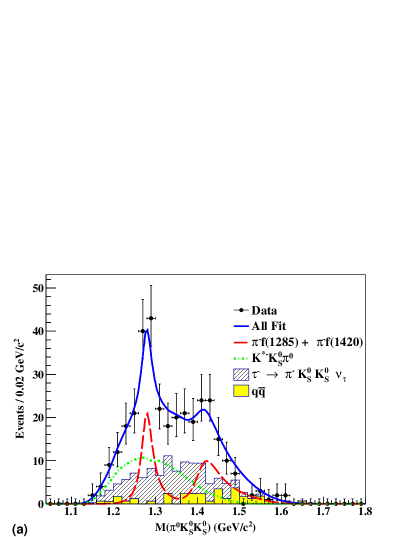
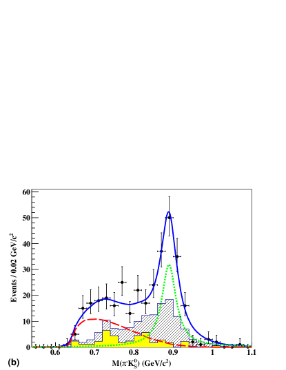
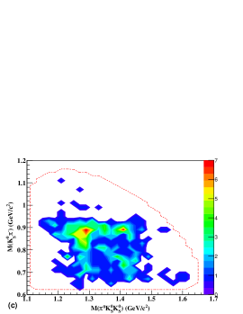
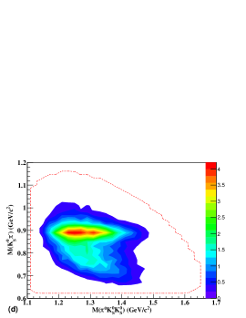
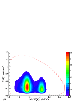
Figure 7: (color online) Invariant mass of the (a) $\pi^{0}K^{0}_{S}K^{0}_{S}$ and (b) $K^{0}_{S}\pi^{-}$ subsystem for $\tau^{-}\rightarrow\pi^{-}K^{0}_{S}K^{0}_{S}\pi^{0}\nu_{\tau}$ candidates. In both histograms, the solid circles with error bars are data, the hatched histogram is the background from $\tau^{-}\to\pi^{-}K^{0}_{S}K^{0}_{S}\nu_{\tau}$, and the shaded (yellow) histogram is the $q\bar{q}$ background. The solid line is the result of the fit with the $\tau^{-}\to f_{1}(1285)\pi^{-}\nu_{\tau}$ +$\tau^{-}\to f_{1}(1420)\pi^{-}\nu_{\tau}$, $\tau^{-}\to K^{*-}K^{0}_{S}\nu_{\tau}$ and background contributions. The $f_{1}(1285)\pi^{-}\nu_{\tau}$ +$f_{1}(1420)\pi^{-}\nu_{\tau}$ and $K^{*-}K^{0}_{S}\nu_{\tau}$ contributions are shown by the dashed (red) and dotted (green) line, respectively. The two-dimensional plot of the invariant masses of $K^{0}_{S}\pi^{-}$ and $\pi^{0}K^{0}_{S}K^{0}_{S}$ system for (c) $\tau^{-}\rightarrow\pi^{-}K^{0}_{S}K^{0}_{S}\pi^{0}\nu_{\tau}$ candidates in data. Two-dimensional plots of the MC events for (d) $\tau^{-}\to K^{*-}K^{0}_{S}\pi^{0}\nu_{\tau}$ and (e) $\tau^{-}\to\pi^{-}f_{1}(1285)\nu_{\tau}+\pi^{-}f_{1}(1420)\nu_{\tau}$ processes. The dotted curve in (c)-(e) shows the kinematic boundary where the invariant mass of the $\pi^{-}K^{0}_{S}K^{0}_{S}\pi^{0}$ system is equal to the $\tau$-lepton mass.

V Mass spectra in the $\tau^{-}\rightarrow\pi^{-}K^{0}_{S}K^{0}_{S}\pi^{0}\nu_{\tau}$ sample

The invariant mass of the $\pi^{0}K^{0}_{S}K^{0}_{S}$ and $K^{0}_{S}\pi^{-}$ subsystem for the $\tau^{-}\rightarrow\pi^{-}K^{0}_{S}K^{0}_{S}\pi^{0}\nu_{\tau}$ selected sample is shown in Fig. 7 (a) and (b), respectively. The $M(\pi^{0}K^{0}_{S}K^{0}_{S})$ distribution in Fig. 7 (a) shows a significant peak at 1280 MeV/$c^{2}$, which is probably due to the $f_{1}(1285)$ resonance. In addition, a small bump-like structure is seen around 1420 MeV/$c^{2}$. The $M(K^{0}_{S}\pi^{-})$ distribution for the same $\tau^{-}\to\pi^{-}K^{0}_{S}K^{0}_{S}\pi^{0}\nu_{\tau}$ sample, in Fig. 7 (b), shows a clear $K^{*}$ peak at 890 MeV/$c^{2}$. These structures are also seen as clear bands in the two-dimensional plot, $M(K^{0}_{S}\pi^{-})$ versus $M(\pi^{0}K^{0}_{S}K^{0}_{S})$, as shown in Fig. 7 (c). It should be noticed that no clear resonance-like structure is observed in the other sub-mass distributions as shown in Fig. 8. In particular, there is no $\rho(770)$ signal in $M(\pi^{-}\pi^{0})$ and no $K^{0*}$ signal in $M(K^{0}_{S}\pi^{0})$. Altogether, this indicates the presence of two dominant components, $\tau^{-}\to\pi^{-}f_{1}(1285)\nu_{\tau}$ and $\tau^{-}\to K^{*-}K^{0}_{S}\pi^{0}\nu_{\tau}$, in the final state of the decay $\tau^{-}\to\pi^{-}K^{0}_{S}K^{0}_{S}\pi^{0}\nu_{\tau}$.

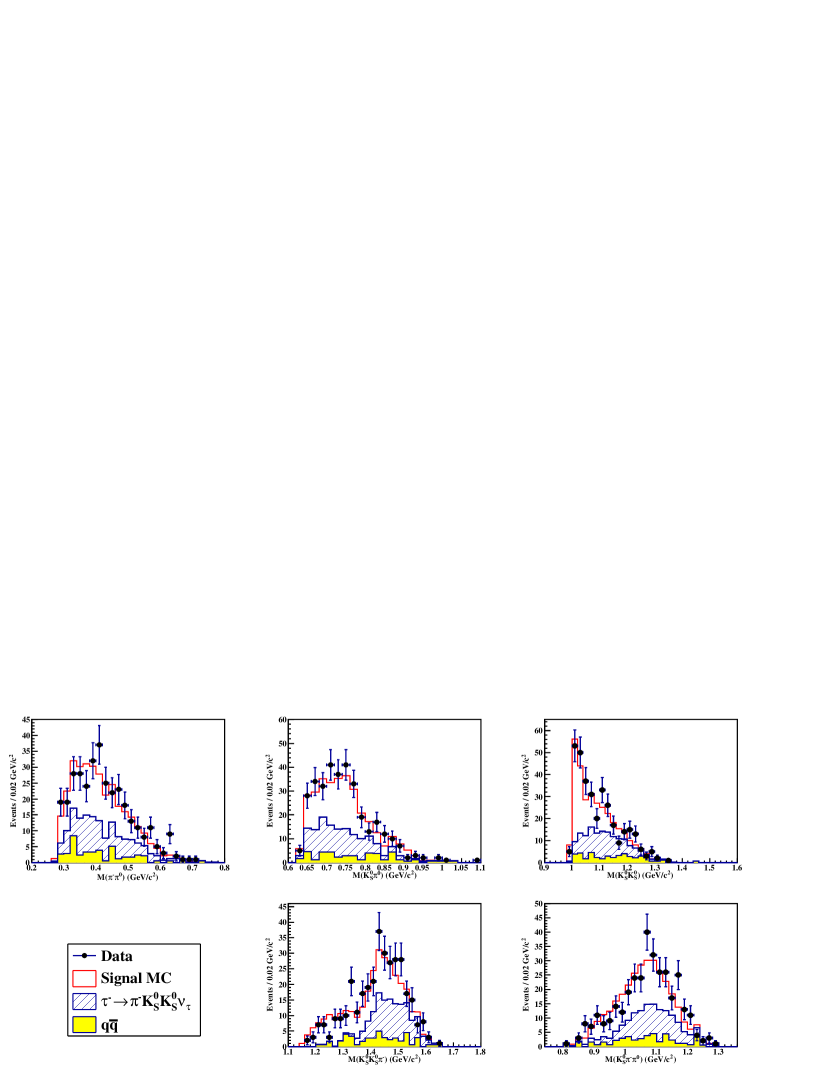
Figure 8: (color online) Invariant mass distributions of the sub-mass systems for $\tau^{-}\to\pi^{-}K^{0}_{S}K^{0}_{S}\pi^{0}\nu_{\tau}$; $M(\pi^{-}\pi^{0})$, $M(K^{0}_{S}\pi^{0})$, $M(K^{0}_{S}K^{0}_{S})$, $M(K^{0}_{S}K^{0}_{S}\pi^{-})$ and $M(K^{0}_{S}\pi^{-}\pi^{0})$. The solid circles with error bars are data. The blank (red) histogram is the sum of the signal $\tau^{-}\rightarrow\pi^{-}K^{0}_{S}K^{0}_{S}\pi^{0}\nu_{\tau}$ and background modeled by MC. The hatched histogram is the background from $\tau^{-}\to\pi^{-}K^{0}_{S}K^{0}_{S}\nu_{\tau}$ and the shaded (yellow) histogram is the $q\bar{q}$ background. See the text for details of the signal model for $\tau^{-}\rightarrow\pi^{-}K^{0}_{S}K^{0}_{S}\pi^{0}\nu_{\tau}$.

In order to make a quantitative evaluation, we perform a simple amplitude analysis assuming incoherent contributions of two intermediate processes $\tau^{-}\to\pi^{-}f_{1}(1285)\nu_{\tau}$ and $\tau^{-}\to K^{*-}K^{0}_{S}\pi^{0}\nu_{\tau}$. In addition, a possible contribution of $f_{1}(1420)$ production through $\tau^{-}\to\pi^{-}f_{1}(1420)\nu_{\tau}$ is also examined.

V.1 Fitting formula

We fit both the $M(\pi^{0}K^{0}_{S}K^{0}_{S})$ and $M(K^{0}_{S}\pi^{-})$ distributions in the decay $\tau^{-}\rightarrow\pi^{-}K^{0}_{S}K^{0}_{S}\pi^{0}\nu_{\tau}$ simultaneously, assuming that the dominant signal processes are those containing intermediate resonances $f_{1}(1285)$, $f_{1}(1420)$ and $K^{*-}$, i.e., $\tau^{-}\to\pi^{-}f_{1}(1285)\nu_{\tau}$, $\tau^{-}\to\pi^{-}f_{1}(1420)\nu_{\tau}$ and $\tau^{-}\to K^{*-}K^{0}_{S}\pi^{0}\nu_{\tau}$. Hereinafter, we refer to these decays as the $f_{1}$, $f^{\prime}_{1}$ and $K^{*-}$ subprocesses, respectively.

We use an unbinned maximum-likelihood fit to extract the resonance parameters in the $M(\pi^{-}K^{0}_{S}K^{0}_{S})$ and $M(K^{0}_{S}\pi^{-})$ distributions. The likelihood function is given by

$$\mathcal{L}= \prod_{i}^{N}\left[f_{f_{1}+f^{\prime}_{1}}\mathcal{P}_{f_{1}+f^{\prime}_{1}}(q_{1,i},q_{2,i};\vec{a})\right.$$

$$+ \left.f_{K^{*-}}\mathcal{P}_{K^{*-}}(q_{1,i},q_{2,i};\vec{a})\right.$$

$$+ \left.(1-f_{f_{1}+f^{\prime}_{1}}-f_{K^{*-}})\mathcal{P}_{B}(q_{1,i},q_{2,i};\vec{a})\right],$$ (11)

where $N$ is the total number of events in the sample, $f_{j}$ is the fraction of the $j$-th category, where the index $j$ stands for $f_{1}+f^{\prime}_{1}$, $K^{*-}$ or the background ($B$) component. $\mathcal{P}_{j}$ is the probability density function (PDF) for the $j$-th component. The variables $q_{1,i}$ and $q_{2,i}$ are the invariant masses of the subsystems, i.e., $q_{1}=M(\pi^{-}K^{0}_{S}K^{0}_{S})$ and $q_{2}=M(K^{0}_{S}\pi^{-})$, for the $i$-th event. The vector $\vec{a}$ represents the resonance shape parameters. We are aware of a possible interference between $f_{1}+f^{\prime}_{1}$ and $K^{*-}$ amplitude; however, our statistics are too low for a quantitative study of this effect and so we ignore it in the fit. We also assume that the PDF is given as the product of individual PDFs for each variables; $\mathcal{P}_{j}=\mathcal{P}_{j}(q_{1})\mathcal{P}_{j}(q_{2})$ for all components ($j=f_{1}+f^{\prime}_{1},K^{*-},$ background). As a result, we have six PDF’s: $\mathcal{P}_{f_{1}+f^{\prime}_{1}}(q_{\alpha})$, $\mathcal{P}_{K^{*-}}(q_{\alpha})$ and $\mathcal{P}_{B}(q_{\alpha})$ for $\alpha=1,2$.

The PDF $\mathcal{P}_{f_{1}+f^{\prime}_{1}}(q_{1})$ is the $M(\pi^{0}K^{0}_{S}K^{0}_{S})$ distribution in the $\tau^{-}\to\pi^{-}f_{1}(1285)(f_{1}(1420))\nu_{\tau}$ decays and is given by

$$\mathcal{P}_{f_{1}+f^{\prime}_{1}}(q_{1})\propto|\beta~{}\textrm{BW}_{f_{1}(1285)}(q^{2}_{1})$$

$$+(1-\beta)~{}\textrm{BW}_{f_{1}(1420)}(q^{2}_{1})|^{2},$$ (12)

where $\textrm{BW}_{X}(s)$ is the relativistic Breit-Wigner function and $\beta$, a ratio of two resonances, is a real number. $\textrm{BW}_{X}(s)$ is defined by

$$\textrm{BW}_{X}(s)=\frac{\sqrt{s}M_{X}}{s-M^{2}_{X}+i\sqrt{s}\Gamma_{X}},$$ (13)

which describes the $f_{1}(1285)$ and $f_{1}(1420)$ resonance shape. $M_{X}$ and $\Gamma_{X}$ are the nominal mass and width for resonance $X$.

For the PDF $\mathcal{P}_{K^{*-}}(q_{2})$, the Breit-Wigner function of Eq. (13) is used to describe the $K^{*-}$ resonance shape in the $M(K^{0}_{S}\pi^{-})$ distribution:

$$\mathcal{P}_{K^{*-}}(q_{2})=|\textrm{BW}_{K^{*-}}(q_{2}^{2})|^{2}.$$

The PDF $\mathcal{P}_{K^{*-}}(q_{1})$ is the $M(\pi^{0}K^{0}_{S}K^{0}_{S})$ distribution for the $\tau^{-}\rightarrow K^{*-}K^{0}_{S}\pi^{0}\nu_{\tau}$ decay. In order to obtain this component, we generate $\tau^{-}\rightarrow K^{*-}K^{0}_{S}\pi^{0}\nu_{\tau}(K^{*-}\to K^{0}_{S}\pi^{-})$ events using PYTHIA 6.4 Sjöstrand et al. (2006), assuming phase space for the $K^{*-}K^{0}_{S}\pi^{0}$ system (see the $K^{*-}K^{0}_{S}\pi^{0}$ contribution in Fig. 7(a)). Note that this distribution is insensitive to the detailed values of the $K^{*}$ resonance parameters. The two-dimensional plot, $M(\pi^{0}K^{0}_{S}K^{0}_{S})$ versus $M(K^{0}_{S}\pi^{-})$, for the $\tau^{-}\to K^{*-}K^{0}_{S}\pi^{0}\nu_{\tau}$ MC events is shown in Fig. 7(d).

The PDF $\mathcal{P}_{f_{1}+f^{\prime}_{1}}(q_{2})$ is the $M(K^{0}_{S}\pi^{-})$ distribution for the $\tau^{-}\to\pi^{-}f_{1}(1285)(f_{1}(1420))\nu_{\tau}$ decays. In order to obtain this component, we generate $\tau^{-}\to\pi^{-}f_{1}(1285)\nu_{\tau}~{}(f_{1}(1285)\to K^{0}_{S}K^{0}_{S}\pi^{0})$ events with the PYTHIA 6.4 code Sjöstrand et al. (2006) and obtain the shape of the $M(K^{0}_{S}\pi^{-})$ distribution (see the $f_{1}(1285)\pi^{-}+f_{1}(1420)\pi^{-}$ contribution in Fig. 7(b)). The same two-dimensional plot for the $\tau^{-}\to\pi^{-}f_{1}(1285)\nu_{\tau}+\pi^{-}f_{1}(1420)\nu_{\tau}$ is shown in Fig. 7(e).

The dominant background for the $\tau^{-}\to\pi^{-}K^{0}_{S}K^{0}_{S}\pi^{0}\nu_{\tau}$ sample is due to the $\tau^{-}\to\pi^{-}K^{0}_{S}K^{0}_{S}\nu_{\tau}$ decay with a fake $\pi^{0}$. In addition, there is a small contribution from the $q\bar{q}$ continuum. In order to model the background component, we tune the mass distribution of the $\tau^{-}\to\pi^{-}K^{0}_{S}K^{0}_{S}\nu_{\tau}$ MC events to agree with the data. The background PDF $\mathcal{P}_{B}(q_{i})$, prepared from the MC prediction, is shown by the shaded histograms of $M(\pi^{-}K^{0}_{S}K^{0}_{S})$ and $M(K^{0}_{S}\pi^{-})$ in Fig. 7(a) and (b), respectively.

V.2 Fit results

The fit results with $f_{1}(1285)\pi^{-}\nu_{\tau}$, $f_{1}(1420)\pi^{-}\nu_{\tau}$, $K^{*-}K^{0}_{S}\pi^{0}\nu_{\tau}$ and background contributions reproduce the data quite well as shown by the solid line in Fig. 7 (a) and (b).

The significance of the $f_{1}(1420)$ component is obtained from the negative log-likelihood difference with and without the $f_{1}(1420)$ signal, $S=-2\rm{ln}(\mathcal{L}_{0}/\mathcal{L}_{\rm max})$, where $\mathcal{L}_{\rm max}$ and $\mathcal{L}_{0}$ is the likelihood with and without the $f_{1}(1420)$ resonance, respectively. We obtain $S=30$ with a change of the number of degrees of freedom by 3. From these results, we conclude that the significance of the $f_{1}(1420)$ is $4.8\sigma$. In the same way, the significances of $f_{1}(1285)$ and $K^{*-}$ are $12\sigma$ and $7.8\sigma$, respectively.

As a result of the fit, the masses and widths for the $f_{1}(1285)$, $f_{1}(1420)$ and $K^{*-}$ are determined to be

$$m_{f_{1}(1285)}=1274\pm 3~{}\textrm{MeV}/c^{2},$$

$$\Gamma_{f_{1}(1285)}=20\pm 4~{}\textrm{MeV}/c^{2},$$

$$m_{f_{1}(1420)}=1425\pm 2~{}\textrm{MeV}/c^{2},$$

$$\Gamma_{f_{1}(1420)}=42\pm 19~{}\textrm{MeV}/c^{2}.$$

$$m_{K^{*-}}=890\pm 3~{}\textrm{MeV}/c^{2},$$

$$\Gamma_{K^{*-}}=48\pm 2~{}\textrm{MeV}/c^{2}.$$

These results are consistent with the world averages Beringer et al. (2012).

The fractions of the three hadronic currents in $\tau^{-}\rightarrow\pi^{-}K^{0}_{S}K^{0}_{S}\pi^{0}\nu_{\tau}$ are determined to be $(34\pm 5)\%$, $(12\pm 3)\%$ and $(54\pm 6)\%$ for the $f_{1}(1285)\pi^{-}\nu_{\tau}$, $f_{1}(1420)\pi^{-}\nu_{\tau}$ and $K^{*-}K^{0}_{S}\pi^{0}\nu_{\tau}$ modes, respectively.

Using the fraction of each component, the products of the branching fractions for the subprocesses are determined to be

$$\mathcal{B}(\tau^{-}\rightarrow f_{1}(1285)\pi^{-}\nu_{\tau})\cdot\mathcal{B}(f_{1}(1285)\to K^{0}_{S}K^{0}_{S}\pi^{0})$$

$$=(0.68\pm 0.13\pm 0.07)\times 10^{-5},$$

$$\mathcal{B}(\tau^{-}\rightarrow f_{1}(1420)\pi^{-}\nu_{\tau})\cdot\mathcal{B}(f_{1}(1420)\to K^{0}_{S}K^{0}_{S}\pi^{0})$$

$$=(0.24\pm 0.05\pm 0.06)\times 10^{-5},$$

$$\mathcal{B}(\tau^{-}\rightarrow K^{*-}K^{0}_{S}\pi^{0}\nu_{\tau})\cdot\mathcal{B}(K^{*-}\to K^{0}_{S}\pi^{-})$$

$$=(1.08\pm 0.14\pm 0.15)\times 10^{-5}.$$

The first uncertainty is statistical and the second is systematic. The systematic uncertainties are estimated by using different fit methods, such as a 1-D fit and a simultaneous fit of two sub-mass distributions. Both statistical and systematical uncertainties of $\mathcal{B}(\tau^{-}\rightarrow\pi^{-}K^{0}_{S}K^{0}_{S}\pi^{0}\nu_{\tau})$ are taken into account as well.

In addition, we examined other subsystems by generating MC events with the ratios of three processes obtained by the above-mentioned fit shown in Fig. 8. The blank histograms (red), the sum of the $f_{1}(1285)\pi^{-}\nu_{\tau}$, $f_{1}(1420)\pi^{-}\nu_{\tau}$, and $K^{*-}K^{0}_{S}\pi^{0}\nu_{\tau}$ processes and the other backgrounds, show the expected distributions of the invariant masses of the other subsystems in the $\tau^{-}\rightarrow\pi^{-}K^{0}_{S}K^{0}_{S}\pi^{0}\nu_{\tau}$ sample. We use the shape of these three processes obtained by PYTHIA 6.4 Sjöstrand et al. (2006) and the fit results for the relative ratio of these components. A small contribution due to the interference between the $f_{1}(1285)$ and $f_{1}(1420)$ resonances is ignored. The invariant mass distributions of all subsystems are explained by this model quite well in our data.

VI Conclusions

Using $616\times 10^{6}$ $\tau^{+}\tau^{-}$ events collected with the Belle detector, we measure the inclusive $K^{0}_{S}$ and six exclusive branching fractions and the covariance matrix for hadronic decays of the $\tau$ lepton containing $K^{0}_{S}$: $\pi^{-}K^{0}_{S}\nu_{\tau}$, $K^{-}K^{0}_{S}\nu_{\tau}$, $\pi^{-}K^{0}_{S}\pi^{0}\nu_{\tau}$, $K^{-}K^{0}_{S}\pi^{0}\nu_{\tau}$, $\pi^{-}K^{0}_{S}K^{0}_{S}\nu_{\tau}$ and $\pi^{-}K^{0}_{S}K^{0}_{S}\pi^{0}\nu_{\tau}$. Our results are summarized in Table 6. The result for $\tau^{-}\to\pi^{-}K^{0}_{S}\nu_{\tau}$ supersedes our previous measurement Epifanov et al. (2007). The accuracy for $\tau^{-}\to K^{-}K^{0}_{S}\nu_{\tau}$, $\tau^{-}\to\pi^{-}K^{0}_{S}\pi^{0}\nu_{\tau}$ and $\tau^{-}\to K^{-}K^{0}_{S}\pi^{0}\nu_{\tau}$ is improved over that of previous experiments by one order of magnitude.

The combined fit of the invariant masses of the $\pi^{0}K^{0}_{S}K^{0}_{S}$ and $\pi^{-}K^{0}_{S}$ system in the $\tau^{-}\rightarrow\pi^{-}K^{0}_{S}K^{0}_{S}\pi^{0}\nu_{\tau}$ events indicates the presence of the $K^{*-}K^{0}_{S}\pi^{0}\nu_{\tau}$, $f_{1}(1285)\pi^{-}\nu_{\tau}$ and $f_{1}(1420)\pi^{-}\nu_{\tau}$ components with significances of 7.8$\sigma$, 12$\sigma$ and 4.8$\sigma$, respectively. Using the branching fractions of the intermediate resonances to the corresponding final states from Beringer et al. (2012), the branching fractions for the $\pi^{-}K^{0}_{S}K^{0}_{S}\pi^{0}\nu_{\tau}$ final state via hadronic currents are determined to be $\mathcal{B}(\tau^{-}\rightarrow f_{1}(1285)\pi^{-}\nu_{\tau})=(0.68\pm 0.13\pm 0.07)\times 10^{-5}$, $\mathcal{B}(\tau^{-}\rightarrow f_{1}(1420)\pi^{-}\nu_{\tau})=(0.24\pm 0.05\pm 0.06)\times 10^{-5}$, and $\mathcal{B}(\tau^{-}\rightarrow K^{*-}K^{0}_{S}\pi^{0}\nu_{\tau})=(1.08\pm 0.14\pm 0.15)\times 10^{-5}$.

VII Acknowledgment

We thank the KEKB group for the excellent operation of the accelerator; the KEK cryogenics group for the efficient operation of the solenoid; and the KEK computer group, the National Institute of Informatics, and the PNNL/EMSL computing group for valuable computing and SINET4 network support. We acknowledge support from the Ministry of Education, Culture, Sports, Science, and Technology (MEXT) of Japan, the Japan Society for the Promotion of Science (JSPS), and the Tau-Lepton Physics Research Center of Nagoya University; the Australian Research Council and the Australian Department of Industry, Innovation, Science and Research; Austrian Science Fund under Grant No. P 22742-N16; the National Natural Science Foundation of China under contract No. 10575109, 10775142, 10825524, 10875115, 10935008 and 11175187; the Ministry of Education, Youth and Sports of the Czech Republic under contract No. MSM0021620859; the Carl Zeiss Foundation, the Deutsche Forschungsgemeinschaft and the VolkswagenStiftung; the Department of Science and Technology of India; the Istituto Nazionale di Fisica Nucleare of Italy; The WCU program of the Ministry Education Science and Technology, National Research Foundation of Korea Grant No. 2011-0029457, 2012-0008143, 2012R1A1A2008330, 2013R1A1A3007772, BRL program under NRF Grant No. KRF-2011-0020333, BK21 Plus program, and GSDC of the Korea Institute of Science and Technology Information; the Polish Ministry of Science and Higher Education and the National Science Center; the Ministry of Education and Science of the Russian Federation, the Russian Federal Agency for Atomic Energy and the RFBR grant 12-02-01032-a; the Slovenian Research Agency; the Basque Foundation for Science (IKERBASQUE) and the UPV/EHU under program UFI 11/55; the Swiss National Science Foundation; the National Science Council and the Ministry of Education of Taiwan; and the U.S. Department of Energy and the National Science Foundation. This work is supported by a Grant-in-Aid from MEXT for Science Research in a Priority Area (“New Development of Flavor Physics”), and from JSPS for Creative Scientific Research (“Evolution of Tau-lepton Physics”).

Appendix

In this appendix, we provide the description of the logarithmic Gaussian that is used to model the $\gamma\gamma$ invariant mass distribution, which is inadequately described with a pure Gaussian distribution. This function is useful for modeling the distribution that has an asymmetrical tail. The normalized logarithmic Gaussian $f(x)$ is given by

$$f(x)=\frac{\eta}{\sqrt{2\pi}\sigma\sigma_{0}}\exp\left(-\frac{\ln^{2}\left(1-\eta(x-x_{p})/\sigma\right)}{2\sigma_{0}^{2}}-\frac{\sigma^{2}_{0}}{2}\right),$$ (14)

where $x_{p}$, $\sigma$ and $\eta$ are free parameters in this function. The parameter $x_{p}$ represents the peak position, $\sigma$ characterizes the mean standard deviation of the distribution and $\eta$ represents the asymmetry of the distribution. As $\eta$ approaches zero, this distribution collapses to a Gaussian. The variable $\sigma_{0}$ is determined by $\eta$ as

$$\sigma_{0}=\frac{2}{\xi}\sinh^{-1}\left(\frac{\eta\xi}{2}\right)$$ (15)

with $\xi=2\sqrt{\ln{4}}\sim 2.35$. The left and right standard deviation ($\sigma_{\pm}$) and the $x$-values ($X_{\pm}$) for which the distribution decreased by a factor of $P$ from the value at the maximum of the distribution are given by

$$\sigma_{\pm} = \pm\frac{\sigma}{\eta}\left(1-e^{\mp\frac{\sigma_{0}\xi}{2}}\right)$$ (16)

$$X_{\pm} = x_{p}+\frac{\sigma}{\eta}\left(1-e^{\mp\sigma_{0}\sqrt{2\ln P}}\right).$$ (17)