The form and the origin of the orbital ordering in the electronic nematic phase of the Iron-based superconductors

Abstract

We investigated the form of the orbital ordering in the electronic nematic phase of the Iron-based superconductors by applying a group theoretical analysis on a realistic five-band model. We find the orbital order can be either of the inter-orbital s-wave form or the intra-orbital d-wave form. From the comparison with existing ARPES measurements of band splitting, we find the orbital ordering in the 122 system is dominated by an intra-orbital d-wave component, while that in the 111 system is dominated by an inter-orbital s-wave component. We find both forms of orbital order are strongly entangled with the nematicity in the spin correlation of the system. The condensation energy of the magnetic ordered phase is found to be significantly improved(by more than 20 percents) when the degeneracy between the $(\pi,0)$ and $(0,\pi)$ ordering pattern is lifted by the orbital order. We argue there should be large difference in both the scattering rate and the size of the possible pseudogap on the electron pocket around the $\mathrm{X}=(\pi,0)$ and $\mathrm{Y}=(0,\pi)$ point in the electronic nematic phase. We propose this as a possible origin for the observed nematicity in resistivity measurements.

The most exciting new feature of the Iron-based superconductors is their multi-orbital nature. Many novel properties of the Iron-based superconductors, especially those with the name of electronic nematicityChuang ; Chu0 ; Chu1 ; Shen0 ; Chu2 ; Kasahara ; Shimojima , have been argued to be related to the orbital physics in these systemsKu ; Lv1 ; Singh ; Lv2 ; Lee1 ; Nevidomskyy ; Chubukov ; Su . The ARPES observation of the rather large splitting between the 3$d_{xz}$ and 3$d_{yz}$-dominated bandShen0 in the magnetic ordered phase further implies that the orbital degree of freedom is deeply involved in the magnetic ordering phase transition. More recent measurements find that the breaking of tetragonal symmetry in the electronic structure can happen even without static magnetic orderingDing ; Matsuda . At the same time, the multi-orbital character is also the key to understand the complex manifestation of electron correlation effect and the structure of superconducting pair in these systemsShen2 ; Kotliar .

However, a comprehensive understanding on the role of orbital degree of freedom in these systems is still in its infancy. In particular, it is still a mystery how the observed electronic nematicity is related to the orbital physics of the system. It is also unclear what is the order parameter for the orbital ordering in the electronic nematic phase of the Iron-based superconductors and how it is entangled with the magnetic, structural and superconducting properties of these systems.

The purpose of this paper is to determine the form of the order parameter for the orbital ordering in the electronic nematic phase of the Iron-based superconductors and explore its physical origin. By applying group theoretical analysis to a realistic five band model derived from band structure calculation, we are able to determine the form of the order parameter for orbital ordering in the electronic nematic phase of the Iron-based superconductors. We find the orbital order can take either an inter-orbital s-wave form or an intra-orbital d-wave form in the space spanned by the degenerate $d_{xz}$ and $d_{yz}$ orbital. From the comparison with ARPES measurements we find the orbital ordering in different families of Iron-based superconductors take different forms. More specifically, while the orbital order in the 122 system is dominated by an intra-orbital d-wave component, the 111 system choose to order mainly in the intra-orbital s-wave channel. We find both types of orbital ordering are strongly entangled with the nematicity of spin correlation in the system and can emerge spontaneously by lifting the degeneracy between the magnetic ordering with wave vector $(\pi,0)$ and $(0,\pi)$. We also argue that there should be large difference in both the scattering rate and the size of pseudogap on the electron pockets around $\mathrm{X}=(\pi,0)$ and $\mathrm{Y}=(0,\pi)$ in the electronic nematic phase. This is proposed to be the physical origin of nematicity observed in resistivity measurementsChu0 ; Chu1 ; Chu2 .

To describe the complex electronic structure in the FeAs plane of the Iron-based superconductors, we adopt the five-band tight binding model derived from first principle calculation of the LaFeAsO systemKuroki . The model reads,

$$H_{band}=\sum_{i,j}\sum_{\mu,\nu,\sigma}t_{i,j}^{\mu,\nu}c_{i,\mu,\sigma}^{\dagger}c_{j,\nu,\sigma}.$$

Here $\mu,\nu=1,..,5$ is the index for the five maximally localized Wannier functions(MLWFs) on the Fe site, namely, $|1\rangle=|3d_{3\mathrm{Z}^{2}-\mathrm{R}^{2}}\rangle$, $|2\rangle=|3d_{\mathrm{XZ}}\rangle$, $|3\rangle=|3d_{\mathrm{YZ}}\rangle$, $|4\rangle=|3d_{\mathrm{X}^{2}-\mathrm{Y}^{2}}\rangle$ and $|5\rangle=|3d_{\mathrm{XY}}\rangle$. $t_{i,j}^{\mu,\nu}$ denotes the hopping integral between the $\mu$-th and $\nu$-th orbital on site $i$ and site $j$. The $\mathrm{X}$ and $\mathrm{Y}$-axis for the Wannier functions are aligned with the Fe-As directions and are rotated by 45 degrees from the $x$ and $y$-axis of the Fe-Fe square lattice.

In the tetragonal phase, the point group around the Fe site is $D_{2d}$, whose generators are $\sigma_{\mathrm{X}}$, $\sigma_{\mathrm{Y}}$ and $R_{x}(\pi)$. Among the five MLWFs, $|3\mathrm{Z}^{2}-\mathrm{R}^{2}\rangle$ belongs to the identity representation, $|\mathrm{XY}\rangle$ and $|\mathrm{X}^{2}-\mathrm{Y}^{2}\rangle$ belong to the one-dimensional $\mathrm{B}_{1}$ and $\mathrm{B}_{2}$ representation, $|\mathrm{XZ}\rangle$ and $|\mathrm{YZ}\rangle$ belong to the two-dimensional representation of the $D_{2d}$ group. If we denote the transformation of five MLWFs under the generators $R_{m}=R_{x}(\pi),\sigma_{\mathrm{X}},\sigma_{\mathrm{Y}}$ as $R_{m}|\mu\rangle=\sum_{\mu^{\prime}}D_{\mu^{\prime},\mu}(R_{m})|\mu^{\prime}\rangle$, then the hopping integrals in the tetragonal phase should satisfy the following equations

$$t_{i,j}^{\mu,\nu}=\sum_{\mu^{\prime},\nu^{\prime}}D_{\mu^{\prime},\mu}(R_{m})D_{\nu^{\prime},\nu}(R_{m})t_{i^{\prime},j^{\prime}}^{\mu^{\prime},\nu^{\prime}},$$ (1)

in which $i^{\prime}=R_{m}^{-1}i$.

In the electronic nematic phase, the local symmetry around each Fe site is reduced to $D_{2}$. In principle, such a symmetry breaking may originate from either the electronic(for example, the charge, spin or orbital degree of freedom) or the lattice degree of freedom. Here we will focus on the symmetry breaking pattern in the orbital space. As a result of this symmetry breaking, additional terms that is forbidden by Eq.(1) can appear in $t_{i,j}^{\mu,\nu}$. These symmetry breaking terms can be interpreted as the order parameter of the orbital order in the electronic nematic phase and can be detected from the band splitting in ARPES measurements. The general form of such symmetry breaking perturbation can be largely determined by group theoretical analysis. Here we will illustrate such a procedure for the on-site symmetry breaking term for clarity.

The basic idea is to distill all the bilinear Hamiltonian terms in the orbital space that is allowed by the symmetry group of the orthogonal phase($D_{2}$) but is forbidden by the symmetry group of the tetragonal phase($D_{2d}$). This can be done by operating the projection operators of the identity representation for the $D_{2d}$ and $D_{2}$ group on an arbitrary initial bilinear Hamiltonian. The $D_{2}$ group has four one dimensional irreducible representations. Among the five MLWFs, $|3\mathrm{Z}^{2}-\mathrm{R}^{2}\rangle$ and $|\mathrm{XY}\rangle$ both belong to the identity representation, $|\mathrm{X}^{2}-\mathrm{Y}^{2}\rangle$ belongs to the $\mathrm{B}_{1}$ representation, the linear combinations $|\mathrm{XZ}\rangle\pm|\mathrm{YZ}\rangle$ belong to the $\mathrm{B}_{2}$ and $\mathrm{B}_{3}$ representations and have the $d_{xz}$ and $d_{yz}$ character. Thus the symmetry allowed on-site Fermion bilinear terms in the orthogonal phase have the general form of

$$H_{2} = \sum_{i,\sigma}(\beta_{1}c^{\dagger}_{i,1,\sigma}c_{i,1,\sigma}+\beta_{2}c^{\dagger}_{i,5,\sigma}c_{i,5,\sigma}+\beta_{3}c^{\dagger}_{i,4,\sigma}c_{i,4,\sigma})$$ (2)

$$+ \beta_{4}\sum_{i,\sigma}(c^{\dagger}_{i,1,\sigma}c_{i,5,\sigma}+c^{\dagger}_{i,5,\sigma}c_{i,1,\sigma})$$

$$+ \beta_{5}\sum_{i,\sigma}(c^{\dagger}_{i,2,\sigma}+c^{\dagger}_{i,3,\sigma})(c_{i,2,\sigma}+c_{i,3,\sigma})$$

$$+ \beta_{6}\sum_{i,\sigma}(c^{\dagger}_{i,2,\sigma}-c^{\dagger}_{i,3,\sigma})(c_{i,2,\sigma}-c_{i,3,\sigma}).$$

However, it can be shown that the bilinear forms $c^{\dagger}_{i,1,\sigma}c_{i,1,\sigma}$, $c^{\dagger}_{i,4,\sigma}c_{i,4,\sigma}$, $c^{\dagger}_{i,5,\sigma}c_{i,5,\sigma}$, and $c^{\dagger}_{i,2,\sigma}c_{i,2,\sigma}+c^{\dagger}_{i,3,\sigma}c_{i,3,\sigma}$ all belong to the identity representation of $D_{2d}$ group. When these symmetric perturbations are removed from Eq.(2), we get the symmetric breaking perturbations in the orthogonal phase, which now takes the simple form of

$$\Delta H = \lambda_{1}\sum_{i,\sigma}(c^{\dagger}_{i,2,\sigma}c_{i,3,\sigma}+c^{\dagger}_{i,3,\sigma}c_{i,2,\sigma})$$

$$+ \lambda_{2}\sum_{i,\sigma}(c^{\dagger}_{i,1,\sigma}c_{i,5,\sigma}+c^{\dagger}_{i,5,\sigma}c_{i,1,\sigma}).$$

Here $\lambda_{1}=\beta_{5}-\beta_{6}$, $\lambda_{2}=\beta_{4}$. If we further restrict our consideration to the subspace spanned by the $d_{\mathrm{XZ}}$ and $d_{\mathrm{YZ}}$ orbital, which are the most relevant degree of freedom in the electronic nematic phase transition, the only allowable on-site symmetry breaking perturbation would be

$$\Delta H = \lambda_{1}\sum_{i,\sigma}(c^{\dagger}_{i,2,\sigma}c_{i,3,\sigma}+c^{\dagger}_{i,3,\sigma}c_{i,2,\sigma}).$$ (3)

The above arguments can be easily generalized to determine the form of the symmetry breaking perturbations on longer distances. The necessity for such nonlocal terms can be seen clearly from the strong momentum dependence of the band splitting observed in ARPES measurements on 122 systemsShen0 . Following the same procedures, we find there are in total 9 independent symmetry breaking perturbations on nearest neighboring Fe-Fe bonds, which can be classified into the extended s-wave, p-wave and d-wave channels,

$$\Delta H=\Delta H_{s}+\Delta H_{p}+\Delta H_{d}.$$

In the subspace spanned by the $d_{\mathrm{XZ}}$ and $d_{\mathrm{YZ}}$ orbital, only an inter-orbital extended s-wave term and an intra-orbital d-wave term are allowed. Combining these terms with the on-site term found above, we find that the symmetry breaking perturbation in the orthogonal phase is given by

$$\Delta H = \eta_{1}\sum_{i,\sigma}(c^{\dagger}_{i,2,\sigma}c_{i,3,\sigma}+c^{\dagger}_{i,3,\sigma}c_{i,2,\sigma})$$ (4)

$$+ \eta_{2}\sum_{i,\delta,\sigma}(c^{\dagger}_{i,2,\sigma}c_{i+\delta,3,\sigma}+c^{\dagger}_{i,3,\sigma}c_{i+\delta,2,\sigma})$$

$$+ \eta_{3}\sum_{i,\delta,\sigma}\mathrm{d}_{\delta}(c^{\dagger}_{i,2,\sigma}c_{i+\delta,2,\sigma}+c^{\dagger}_{i,3,\sigma}c_{i+\delta,3,\sigma}).$$

Here $\delta$ denotes the vectors connecting nearest neighboring Fe sites and $\mathrm{d}_{\delta}$ is the d-wave form factor. In principle, symmetry breaking terms on longer bonds can also be determined in the same manner. However, from the comparison with the ARPES measurements, we find it suffices to keep only the on-site and the nearest neighboring terms. A list of all independent symmetry breaking terms up to the next nearest neighboring bonds is given in the appendix for reference.

The three parameters $\eta_{1,2,3}$ in Eq.(4) can be determined from fitting the momentum dependence of the band splitting found in ARPES measurements. In particular, they can be extracted from the band splitting at the high symmetry momentum of $\Gamma=(0,0)$, $\mathrm{X}=(\pi,0)$, $\mathrm{Y}=(0,\pi)$ and $\mathrm{M}=(\pi,\pi)$. From group theoretical point of view, the electronic state at these high symmetry momentums should form the basis functions of irreducible representation of the $D_{2}$ group, which is also the wave vector point group at these momentums in the electronic nematic phase. Thus, the electronic state in the $3d_{xz}$ and $3d_{yz}$-dominated bands should have pure $d_{xz}$ and $d_{yz}$ character at these momentums. The band splitting at these momentums are given by

$$\Delta E_{d_{xz}}(\Gamma) = \eta_{1}+4\eta_{2},\ \Delta E_{d_{yz}}(\Gamma)=-\eta_{1}-4\eta_{2}$$

$$\Delta E_{d_{xz}}(\mathrm{X}) = \eta_{1}-4\eta_{3},\ \Delta E_{d_{yz}}(\mathrm{X})=-\eta_{1}-4\eta_{3}$$

$$\Delta E_{d_{xz}}(\mathrm{Y}) = \eta_{1}+4\eta_{3},\ \Delta E_{d_{yz}}(\mathrm{Y})=-\eta_{1}+4\eta_{3}$$

$$\Delta E_{d_{xz}}(\mathrm{M}) = \eta_{1}-4\eta_{2},\ \Delta E_{d_{yz}}(\mathrm{M})=-\eta_{1}+4\eta_{2}$$

Since the $3d_{xz}$ and $3d_{yz}$-dominated bands are far away from the Fermi level around the $\mathrm{M}$ point, we will focus on the band splitting along the $\Gamma-\mathrm{X}$ and $\Gamma-\mathrm{Y}$ directions in the following.

The momentum dependence of the band splitting induced by the three types of orbital orders are plotted in Fig.1. To see the band splitting more clearly, we overlay the dispersion along the $\Gamma-\mathrm{Y}$ direction on that along the $\Gamma-\mathrm{X}$ direction. In the tetragonal phase, the dispersion of the $3d_{yz}$-dominated band along the $\Gamma-\mathrm{X}$ direction should be identical with that of the $3d_{xz}$-dominated band along the $\Gamma-\mathrm{Y}$ direction, which are plotted as thin lines in Fig.1 for reference. The band splitting caused by the on-site orbital order is nonzero in the whole Brillouin zone and is only weakly momentum dependent. For the extended s-wave orbital order, the band splitting reaches its maximum(denoted as $\Delta_{max}$) at the $\Gamma$ point and is exactly zero at the $\mathrm{X}$ and $\mathrm{Y}$ points. For the d-wave orbital order, the band splitting vanishes at the $\Gamma$ point and $\Delta_{max}$ is reached at the $\mathrm{X}$ and $\mathrm{Y}$ points.

We now compare the theoretical predictions with the ARPES measurements. In the Co-doped Ba122 system, the observed band splitting in the $\Gamma-\mathrm{X}$ and $\Gamma-\mathrm{Y}$ direction exhibits strong momentum dependence and is very similar to the d-wave from presented above. In particular, the band splitting is negligible small around the $\Gamma$ point but is the most evident at the $\mathrm{X}$ and $\mathrm{Y}$ pointsShen0 . On the other hand, in both the Na111 system or Li111 system, the observed band splitting is clearly nonzero at the $\Gamma$ point and the momentum dependence along the $\Gamma-\mathrm{X}$ and $\Gamma-\mathrm{Y}$ direction is much less pronounced than that in Co-doped Ba122 systemFeng ; Shen1 ; Ding . Thus the order parameter for orbital ordering in the 111 systems is more likely of the on-site form. In principle, an extended s-wave component is also possible in the 111 system. However, as we will show below, the appearance of the extended-s-wave component is very unlikely from energetic considerations. Thus, the form of orbital ordering in the iron-based superconductors depends on the family of the material studied. It is interesting to know if there is any generic reason that the Co-doped Ba122 system and the Na111 system or Li111 system choose different orbital ordering patterns.

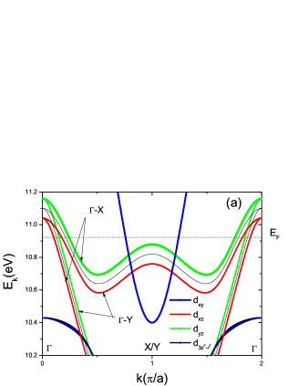
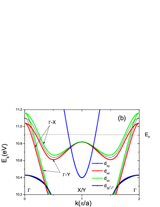
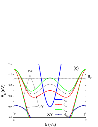
Figure 1: Overlay of the band dispersion along the $\Gamma-\mathrm{X}$ direction on that along the $\Gamma-\mathrm{Y}$ direction. The dominant orbital character is indicated by the color of the lines and the dispersion in the tetragonal phase is plotted in thin lines for reference. In the calculation we have set $(\eta_{1},\eta_{2},\eta_{3})=(60,0,0)$ meV for the on-site case(a), $(0,15,0)$ meV for the extended s-wave case(b) and $(0,0,30)$ meV for the d-wave case(c). The dashed line indicates the Fermi level at $n=6.1$.

Now we discuss the possible origin of the orbital ordering in the Iron-based superconductors. From the point of view of symmetry, the orbital ordering in the electronic nematic phase can be just a secondary effect caused by the breaking of tetragonal symmetry in other channels such as the spin, charge or lattice degree of freedom and has little contribution to the condensation energy of the ordered phase. Here we will adopt a more exotic point of view and assume that the orbital ordering can contribute significantly to the condensation energy of the electronic nematic phase and thus emerge spontaneously. This is a reasonable assumption since the size of the observed band splitting in the electronic nematic phase is already comparable to or even larger than the energy scales of other major ordering tendencies in the system such as SDW order and superconductivity. However, RPA calculations on the five band model indicates that the Iron-based superconductors are far from a pure orbital ordering instability. To resolve this problem, we assume that the orbital ordering is strongly entangled with the nematicity of spin correlation in the Iron-based superconductors, which is dominated by two degenerate channels with wave vector $(\pi,0)$ and $(0,\pi)$. As we will show below, the orbital order can lift such a degeneracy and help the system to gain significantly more condensation energy by selecting the favored ordering wave vector in a way similar to the conventional Jahn-Teller effect.

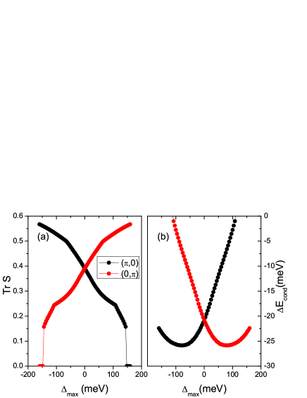
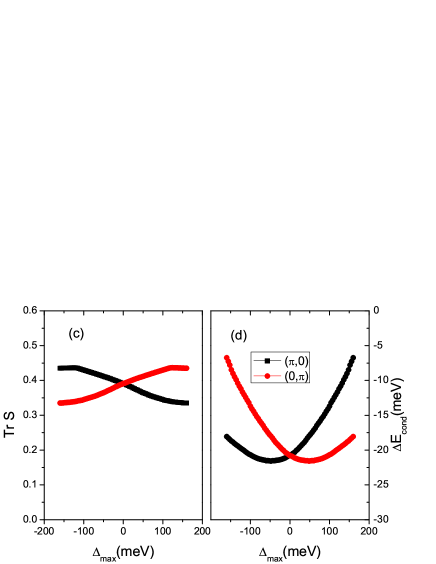
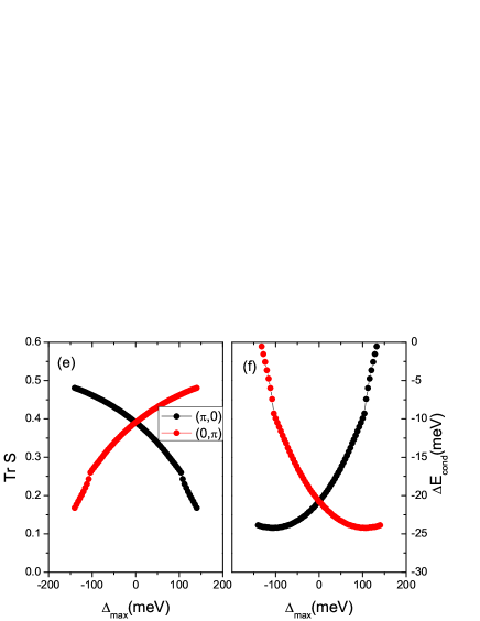
Figure 2: Selection of SDW ordering pattern by orbital ordering. Left: the ordered moment in the presence of on-site(a), extended s-wave(c) and d-wave(e) orbital order. Right: the condensation energy per unit cell in the presence of on-site(b), extended s-wave(d) and d-wave(f) orbital order.

In the following, we will illustrate the coupling between the orbital order and the nematicity in the spin correlation at the mean field level for the SDW ordered state. For this purpose, we introduce the standard Kanamori-Hubbard Hamiltonian for the on-site interactions on the Fe site. We then solve the mean filed equations for the SDW order parameters in the presence of orbital order. The SDW order is assumed to be collinear and has wave vector of either $\mathrm{Q}_{x}=(\pi,0)$ or $\mathrm{Q}_{y}=(0,\pi)$. More specifically, the SDW order parameter is assumed to be of the form $\langle\frac{1}{2}\sum_{\sigma}\sigma c^{\dagger}_{i,\mu,\sigma}c_{i,\nu,\sigma}\rangle=e^{i\mathrm{Q}_{x,y}\cdot\mathrm{R}_{i}}S_{\mu,\nu}$, in which $S_{\mu,\nu}$ is a $5\times 5$ matrix describing the distribution of the magnetic moment in the orbital space. In the following, we will adopt $\mathrm{Tr}S=\sum_{\mu}S_{\mu,\mu}$ as a measure of the magnitude of the ordered moment. In the calculation, we set the interaction strength as $U=1.5$eV, $U^{\prime}=1.0$eV and $J_{H}=0.25$eV, which is large enough to induce a moderate-sized ordered moment. The electron density is fixed at $n=6.0$ in the calculation.

The solution to the mean field self-consistent equations is shown in Fig.2. We find all the three types of orbital ordering can couple to the nematicity in spin correlation. However, the strengthes of the coupling are quite different for the three types of orbital ordering. In particular, the coupling of the extended s-wave orbital order to the nematicity of spin correlation is much weaker than that of the on-site and the d-wave orbital order. For both the on-site and the d-wave orbital order, the disfavored ordering pattern is totally suppressed when the maximal band splitting $\Delta_{max}$ exceeds 160 meV, while in the case of the extended s-wave orbital order, the change in the size of ordered moment is less than 20 percent even for $\Delta_{max}=200meV$. To see if the orbital order can emerge spontaneously from such a coupling, we calculate the condensation energy of the system as a function of the orbital order, which is also shown in Fig.2. We find both the on-site and the d-wave orbital order can improve the condensation energy significantly(more than 20 percents) and a sizeable orbital order can be stabilized in both channels. On the other hand, the improvement to the condensation energy from the extended s-wave orbital order is rather small and the induced orbital order is also much smaller than that in the other two channels.

Such a difference in the coupling strength can be understood intuitively in the weak coupling picture from the nesting property of the Fermi surface, which is important for the spin correlation. More specifically, the band splitting between the $\mathrm{X}$ and the $\mathrm{Y}$ point will enhance the nesting of the electron pocket(with the hole pocket around the $\Gamma$ point) around one of these two momentums and suppress the nesting of the electron pocket around the other momentum. However, in the extended s-wave channel, the band splitting is suppreseed around the $\mathrm{X}$ and the $\mathrm{Y}$ point. This explains its weak entanglement with the nematicity in the spin correlation. Since the orbital order can make such a significant contribution to the condensation energy of the ordered phase, it is more reasonable to think of the orbital order as a component of a composite order parameter involving both the spin and the orbital degree of freedom, rather than a secondary effect of magnetic ordering.

We note the entanglement between the orbital order and the nematicity in spin correlation is not limited in the magnetic ordered phase. In the paramagnetic phase, such a coupling can be realized through the so called Aslamazov-Larkin type vertex correctionKontani . A recent ARPES study of the BaFe₂(AsP)₂ has found simultaneously the evidence of pseudogap opening on the Fermi surface, which is most likely due to strong scattering with spin fluctuation, and the band splitting between the $\mathrm{X}$ and $\mathrm{Y}$ point in the electronic nematic phase of the systemMatsuda . Following our line of reasoning, we should expect rather different scattering rate and different size of the pseudogap on the electron pocket around the $\mathrm{X}$ and $\mathrm{Y}$ point in the electronic nematic phase of the Iron-based superconductors. We propose this as a possible origin for the observed nematicity in resistivity measurements in the electronic nematic phase.

In conclusion, by applying group theoretical analysis to a realistic five band model, we have determined the form of the orbital ordering in the electronic nematic phase of the Iron-based superconductors. We find the orbital ordering in these systems can be either of the inter-orbital s-wave form or the intra-orbital d-wave form. From the comparison with the ARPES observations, we find the orbital ordering in the 122 systems is dominated by the intra-orbital d-wave component, while that in the 111 systems is better described with an on-site intra-orbital form. From a mean field calculation, we find both types of orbital ordering are strongly entangled with the nematicity of the spin correlation and can emerge spontaneously in the model we have studied. We find the orbital order can contribute significantly to the condensation energy of the magnetic ordered phase and it is thus more reasonable to think of the orbital order as a component of a composite order parameter involving both the spin and the orbital degree of freedom, rather than a secondary effect of magnetic ordering. We predict that both the scattering rate and the size of pseudogap should be quite different on the electron pocket around the $\mathrm{X}$ and $\mathrm{Y}$ point in the electronic nematic phase of the Iron-based superconductors. We propose this as a possible origin for the observed nematicity in resistivity measurements in the electronic nematic phase.

Yuehua Su is support by NSFC Grant No. 10974167 and Tao Li is supported by NSFC Grant No. 10774187, No. 11034012 and National Basic Research Program of China No. 2010CB923004. We are grateful to K. Kuroki for clarifying the phase convention used in Ref.Kuroki, .

I Appendix

In this appendix, we present all possible symmetry breaking terms in the electronic nematic phase in the full five dimensional orbital space up to the next nearest neighboring bonds. Here we will assume that both the translational and the time reversal symmetry is respected in the electronic nematic phase. Following the procedure as outlined in the main text, we find there are in total 9 independent symmetry breaking perturbations on nearest neighboring Fe-Fe bonds and 6 independent symmetry breaking perturbations on the next nearest neighboring bonds. The form of the symmetry breaking terms on the nearest neighboring bonds are given by

$$\Delta H=\Delta H_{s}+\Delta H_{p}+\Delta H_{d},$$

in which

$$\Delta H_{s} = \kappa_{1}\sum_{i,\delta,\sigma}(c^{\dagger}_{i,2,\sigma}c_{i+\delta,3,\sigma}+c^{\dagger}_{i,3,\sigma}c_{i+\delta,2,\sigma})$$

$$+ \kappa_{2}\sum_{i,\delta,\sigma}(c^{\dagger}_{i,1,\sigma}c_{i+\delta,5,\sigma}+c^{\dagger}_{i,5,\sigma}c_{i+\delta,1,\sigma})$$

$$\Delta H_{p} = \kappa_{3}\sum_{i,\delta,\sigma}(\mathrm{p}_{\delta}c^{\dagger}_{i,1,\sigma}c_{i+\delta,2,\sigma}+\mathrm{p}^{\prime}_{\delta}c^{\dagger}_{i,1,\sigma}c_{i+\delta,3,\sigma})$$

$$+ \kappa_{3}\sum_{i,\delta,\sigma}(\mathrm{p}_{\delta}c^{\dagger}_{i,2,\sigma}c_{i+\delta,1,\sigma}+\mathrm{p}^{\prime}_{\delta}c^{\dagger}_{i,3,\sigma}c_{i+\delta,1,\sigma})$$

$$+ \kappa_{4}\sum_{i,\delta,\sigma}(\mathrm{p}_{\delta}c^{\dagger}_{i,3,\sigma}c_{i+\delta,5,\sigma}+\mathrm{p}^{\prime}_{\delta}c^{\dagger}_{i,2,\sigma}c_{i+\delta,5,\sigma})$$

$$+ \kappa_{4}\sum_{i,\delta,\sigma}(\mathrm{p}_{\delta}c^{\dagger}_{i,5,\sigma}c_{i+\delta,3,\sigma}+\mathrm{p}^{\prime}_{\delta}c^{\dagger}_{i,5,\sigma}c_{i+\delta,2,\sigma})$$

$$+ \kappa_{5}\sum_{i,\delta,\sigma}(\mathrm{p}_{\delta}c^{\dagger}_{i,2,\sigma}c_{i+\delta,4,\sigma}-\mathrm{p}^{\prime}_{\delta}c^{\dagger}_{i,3,\sigma}c_{i+\delta,4,\sigma})$$

$$+ \kappa_{5}\sum_{i,\delta,\sigma}(\mathrm{p}_{\delta}c^{\dagger}_{i,4,\sigma}c_{i+\delta,2,\sigma}-\mathrm{p}^{\prime}_{\delta}c^{\dagger}_{i,4,\sigma}c_{i+\delta,3,\sigma}),$$

and

$$\Delta H_{d} = \kappa_{6}\sum_{i,\delta,\sigma}\mathrm{d}_{\delta}(c^{\dagger}_{i,2,\sigma}c_{i+\delta,2,\sigma}+c^{\dagger}_{i,3,\sigma}c_{i+\delta,3,\sigma})$$

$$+ \kappa_{7}\sum_{i,\delta,\sigma}\mathrm{d}_{\delta}c^{\dagger}_{i,1,\sigma}c_{i+\delta,1,\sigma}$$

$$+ \kappa_{8}\sum_{i,\delta,\sigma}\mathrm{d}_{\delta}c^{\dagger}_{i,4,\sigma}c_{i+\delta,4,\sigma}$$

$$+ \kappa_{9}\sum_{i,\delta,\sigma}\mathrm{d}_{\delta}c^{\dagger}_{i,5,\sigma}c_{i+\delta,5,\sigma}$$

represent the extended s-wave, p-wave and d-wave components of the symmetry breaking perturbations. Here $\mathrm{p}_{\delta}$, $\mathrm{p^{\prime}}_{\delta}$ are p-wave form factors, $\mathrm{d}_{\delta}$ is the d-wave form factor. The value of these form factors are illustrated in Fig.3.

Figure 3: An illustration of the p-wave and d-wave form factors on the nearest neighboring bonds.

In the subspace spanned by the $d_{\mathrm{XZ}}$ and $d_{\mathrm{YZ}}$ orbital, there are only two possible terms on the nearest neighboring bond and are given by

$$\Delta H = \eta_{2}\sum_{i,\delta,\sigma}(c^{\dagger}_{i,2,\sigma}c_{i+\delta,3,\sigma}+c^{\dagger}_{i,3,\sigma}c_{i+\delta,2,\sigma})$$ (6)

$$+ \eta_{3}\sum_{i,\delta,\sigma}\mathrm{d}_{\delta}(c^{\dagger}_{i,2,\sigma}c_{i+\delta,2,\sigma}+c^{\dagger}_{i,3,\sigma}c_{i+\delta,3,\sigma})$$

in which $\eta_{2}=\kappa_{1}$, $\eta_{3}=\kappa_{6}$.

The 6 allowed symmetry breaking perturbations on the next nearest neighboring bonds are given by

$$\Delta H^{\prime}=\Delta H^{\prime}_{s}+\Delta H^{\prime}_{p}+\Delta H^{\prime}_{d},$$

in which

$$\Delta H^{\prime}_{s} = \kappa^{\prime}_{1}\sum_{i,\delta^{\prime},\sigma}(c^{\dagger}_{i,1,\sigma}c_{i+\delta^{\prime},5,\sigma}+c^{\dagger}_{i,5,\sigma}c_{i+\delta^{\prime},1,\sigma})$$

$$+ \kappa^{\prime}_{2}\sum_{i,\delta^{\prime},\sigma}(c^{\dagger}_{i,2,\sigma}c_{i+\delta^{\prime},3,\sigma}+c^{\dagger}_{i,3,\sigma}c_{i+\delta^{\prime},2,\sigma})$$

$$\Delta H^{\prime}_{p} = \kappa^{\prime}_{3}\sum_{i,\delta^{\prime},\sigma}(\mathrm{p}_{\delta^{\prime}}c^{\dagger}_{i,1,\sigma}c_{i+\delta^{\prime},2,\sigma}+\mathrm{p}^{\prime}_{\delta^{\prime}}c^{\dagger}_{i,1,\sigma}c_{i+\delta^{\prime},3,\sigma})$$

$$+ \kappa^{\prime}_{3}\sum_{i,\delta^{\prime},\sigma}(\mathrm{p}_{\delta^{\prime}}c^{\dagger}_{i,2,\sigma}c_{i+\delta^{\prime},1,\sigma}+\mathrm{p}^{\prime}_{\delta^{\prime}}c^{\dagger}_{i,3,\sigma}c_{i+\delta^{\prime},1,\sigma})$$

$$+ \kappa^{\prime}_{4}\sum_{i,\delta^{\prime},\sigma}(\mathrm{p}_{\delta^{\prime}}c^{\dagger}_{i,3,\sigma}c_{i+\delta^{\prime},5,\sigma}+\mathrm{p}^{\prime}_{\delta^{\prime}}c^{\dagger}_{i,2,\sigma}c_{i+\delta^{\prime},5,\sigma})$$

$$+ \kappa^{\prime}_{4}\sum_{i,\delta^{\prime},\sigma}(\mathrm{p}_{\delta^{\prime}}c^{\dagger}_{i,5,\sigma}c_{i+\delta^{\prime},3,\sigma}+\mathrm{p}^{\prime}_{\delta^{\prime}}c^{\dagger}_{i,5,\sigma}c_{i+\delta^{\prime},2,\sigma})$$

$$+ \kappa^{\prime}_{5}\sum_{i,\delta^{\prime},\sigma}(\mathrm{p}_{\delta^{\prime}}c^{\dagger}_{i,2,\sigma}c_{i+\delta^{\prime},4,\sigma}-\mathrm{p}^{\prime}_{\delta^{\prime}}c^{\dagger}_{i,3,\sigma}c_{i+\delta^{\prime},4,\sigma}),$$

$$+ \kappa^{\prime}_{5}\sum_{i,\delta^{\prime},\sigma}(\mathrm{p}_{\delta^{\prime}}c^{\dagger}_{i,4,\sigma}c_{i+\delta^{\prime},2,\sigma}-\mathrm{p}^{\prime}_{\delta^{\prime}}c^{\dagger}_{i,4,\sigma}c_{i+\delta^{\prime},3,\sigma})$$

and

$$\Delta H^{\prime}_{d} = \kappa^{\prime}_{6}\sum_{i,\delta^{\prime},\sigma}\mathrm{d}_{\delta^{\prime}}(c^{\dagger}_{i,4,\sigma}c_{i+\delta^{\prime},5,\sigma}+c^{\dagger}_{i,5,\sigma}c_{i+\delta^{\prime},4,\sigma}).$$

Here $\delta^{\prime}$ denote the vectors connecting next nearest neighboring Fe sites and $\mathrm{p}_{\delta^{\prime}}$, $\mathrm{p}^{\prime}_{\delta^{\prime}}$ and $\mathrm{d}_{\delta^{\prime}}$ are the p-wave and the d-wave form factor on next nearest neighboring bonds, which are illustrated in Fig.4. In the subspace spanned by the $d_{\mathrm{XZ}}$ and $d_{\mathrm{YZ}}$ orbital, there is only one allowable symmetry breaking perturbation on the next nearest neighboring bonds, which has the form of

$$\Delta H = \eta_{4}\sum_{i,\delta^{\prime},\sigma}(c^{\dagger}_{i,2,\sigma}c_{i+\delta^{\prime},3,\sigma}+c^{\dagger}_{i,3,\sigma}c_{i+\delta^{\prime},2,\sigma}).$$

Here $\eta_{4}=\kappa^{\prime}_{2}$.

Figure 4: An illustration of the p-wave and d-wave form factors on the next nearest neighboring bonds.

References

- (1) T.M. Chuang, M.P. Allan, J. Lee, Y. Xi, N. Ni, S. Bud’ko, G.S. Boebinger, P.C. Canfield, and J.C. Davis, Science 327, 181 (2010).
- (2) J.H. Chu, J.G. Analytis, D. Press, K. De Greve, T.D. Ladd, Y. Yamamoto, and I.R. Fisher, Phys. Rev. B 81, 214502 (2010).
- (3) J.H. Chu, J.G. Analytis, K. De Greve, P.L. McMahon, Z. Islam, Y. Yamamoto, and I.R. Fisher, Science 329, 824 (2010).
- (4) M. Yi, D. Lu, J.H. Chu, J. Analytis, A. Sorini, A. Kemper, B. Moritz, S.K. Mo, R.G. Moore, M. Hashimoto, W.S. Lee, Z. Hussain, T. Devereaux, I.R. Fisher, and Z.X. Shen, Proc. Natl. Acad. Sci. 108, 6878 (2011).
- (5) J.H. Chu, H.H. Kuo, J.G. Analytis and I.R. Fisher, Science 337, 710 (2012).
- (6) S. Kasahara, H. J. Shi, K. Hashimoto, S. Tonegawa, Y. Mizukami, T. Shibauchi, K. Sugimoto, T. Fukuda, T. Terashima, A.H. Nevidomskyy and Y. Matsuda Nature 486, 382 (2012).
- (7) T. Shimojima, K. Ishizaka, Y. Ishida, N. Katayama, K. Ohgushi, T. Kiss, M. Okawa, T. Togashi, X.-Y. Wang, C.-T. Chen, S. Watanabe, R. Kadota, T. Oguchi, A. Chainani and S. Shin, Phys. Rev. Lett. 104, 057002 (2010).
- (8) C.C. Lee, W.G. Yin and W. Ku, Phys. Rev. Lett. 103, 267001 (2009).
- (9) W. Lv, J. Wu, and P. Phillips, Phys. Rev. B 80, 224506 (2009).
- (10) C.C. Chen, J. Maciejko, A.P. Sorini, B. Moritz, R.R.P. Singh and T. P. Devereaux, Phys. Rev. B 82, 100504 (2010).
- (11) W. Lv, F. Kruger, and P. Phillips, Phys. Rev. B 82, 045125 (2010).
- (12) W.C. Lee, W. Lv, J. M. Tranquada, and P. W. Phillips, Phys. Rev. B 86, 094516 (2012).
- (13) A. H. Nevidomskyy, arxiv.org:1104.1747 (2011).
- (14) R. M. Fernandes, A. V. Chubukov, J. Knolle, I. Eremin, and J. Schmalian, Phys. Rev. B 85, 024534 (2012).
- (15) Y.H. Su and T. Li, arXiv:1303.7302.
- (16) M. Yi, D. Lu, R. Yu, S.C. Riggs, J.H. Chu, B. Lv, Z.K. Liu, M. Lu, Y.T. Cui, M. Hashimoto, S.K. Mo, Z. Hussain, C.W. Chu, I.R. Fisher, Q. Si and Z.X. Shen, Phys. Rev. Lett. 110, 067003(2013).
- (17) Z. P. Yin, K. Haule and G. Kotliar, arXiv:1311.1188.
- (18) Y. Zhang, F. Chen, C. He, B. Zhou, B. P. Xie, C. Fang, W. F. Tsai, X. H. Chen, H. Hayashi, J. Jiang, H. Iwasawa, K. Shimada, H. Namatame, M. Taniguchi, J. P. Hu, D. L. Feng, Phys. Rev. B 83, 054510 (2011).
- (19) M. Yi, D. H. Lu, R. G. Moore, K. Kihou, C.-H. Lee, A. Iyo, H. Eisaki, T. Yoshida, A. Fujimori and Z.-X. Shen, NJP 14, 073019 (2012).
- (20) T. Shimojima, T. Sonobe, W. Malaeb, K. Shinada, A. Chainani, S. Shin, T. Yoshida, S. Ideta, A. Fujimori, H. Kumigashira, K Ono, Y. Nakashima, H. Anzai, M. Arita, A. Ino, H. Namatame, M. Taniguchi, M. Nakajima, S. Uchida, Y. Tomioka, T.Ito, K. Kihou, C. H. Lee, A. Iyo, H. Eisaki, K. Ohgushi, S. Kasahara, T. Terashima, H. Ikeda, T. Shibauchi, Y. Matsuda and K. Ishizaka Phys. Rev. B 89, 045101 (2014).
- (21) H. Miao, L. -M. Wang, P. Richard, S. -F. Wu, J. Ma, T. Qian, L. -Y. Xing, X. -C. Wang, C. -Q. Jin, C. -P. Chou, Z. Wang, W. Ku, H. Ding, arXiv:1310.4601.
- (22) K. Kuroki, S. Onari, R. Arita, H. Usui, Y. Tanaka, H. Kontani, and H. Aoki, Phys. Rev. Lett.101, 087004 (2008).
- (23) S. Onari and H. Kontani, Phys. Rev. Lett. 109 , 137001 (2012).