Synchronization-Free Delay Tomography
Based on Compressed Sensing

Abstract

Delay tomography has so far burdened source and receiver measurement nodes in a network with two requirements such as path establishment and clock synchronization between them. In this letter, we focus on the clock synchronization problem in delay tomography and propose a synchronization-free delay tomography scheme. The proposed scheme selects a path between source and receiver measurement nodes as a reference path, which results in a loss of equation in a conventional delay tomography problem. However, by utilizing compressed sensing, the proposed scheme becomes robust to the loss. Simulation experiments confirm that the proposed scheme works comparable to a conventional delay tomography scheme in networks with no clock synchronization between source and receiver measurement nodes.

I Introduction

Delay tomography means to estimate internal link delays in a network by means of measuring end-to-end path delays [1]. When an active measurement procedure is used, source measurement nodes transmit probe packets to receiver measurement nodes, and the end-to-end path delays are computed from the differences between the transmission and reception times of the probe packets.

So far, delay tomography has burdened source and receiver measurement nodes with two requirements; path establishment and clock synchronization between them. In this letter, we focus on the clock synchronization problem in delay tomography and propose a synchronization-free delay tomography scheme. Although there have been several works for the path establishment problem [2], to the best of the authors’ knowledge, the clock synchronization problem has not been studied so far.

The proposed scheme utilizes compressed sensing, which is a promising technique because it can reduce the number of paths between source and receiver measurement nodes [3, 4], and identifies bottleneck links without any clock synchronization mechanism between them. In the proposed scheme, we construct a differential routing matrix by setting a path between source and receiver measurement nodes as a reference path, so it results in a loss of equation for the delay tomography problem. Since compressed sensing is robust to this problem, however, the proposed scheme works comparable to a conventional delay tomography scheme in networks with no clock synchronization between source and receiver measurement nodes.

The proposed scheme has a significant benefit in various network environments especially in wireless networks such as wireless sensor networks, in which electronic components of nodes are sometimes too untrustable to meet the requirement of clock synchronization in terms of accuracy and complexity. In addition, it gives an insight to general problems of compressed sensing in which measurement process has an unknown bias.

II Preliminary for Compressed Sensing

First, we define the $\ell_{p}$ norm ($p\geq 1$) of a vector $\mathbf{x}=[x_{1}~{}x_{2}~{}\cdots~{}x_{N}]^{\top}\in\mathcal{R}^{N}$ as

$$\|\mathbf{x}\|_{p}=\Bigl{(}\sum_{i=1}^{N}|x_{i}|^{p}\Bigr{)}^{\frac{1}{p}},$$ (1)

where $\top$ denotes the transpose operator.

Now, we assume that through a matrix $\mathbf{A}\in\mathcal{R}^{M\times N}$ ($M<N$), a vector $\mathbf{y}=[y_{1}~{}y_{2}~{}\cdots~{}y_{M}]^{\top}\in\mathcal{R}^{M}$ is obtained for a vector $\mathbf{x}$ as $\mathbf{y}=\mathbf{A}\mathbf{x}$. When utilizing compressed sensing, whether or not one can recover a sparse vector $\mathbf{x}$ from $\mathbf{y}$ depends on the mathematical property of $\mathbf{A}$. Here, we define the mutual coherence $\mu(\mathbf{A})$, which can provide guarantees of the recovery of the sparse vector, as

$$\mu(\mathbf{A})=\max_{1\leq j,j^{\prime}\leq N,j\neq j^{\prime}}\frac{|\mathbf{a}_{j}^{\top}\mathbf{a}_{j^{\prime}}|}{\|\mathbf{a}_{j}\|_{2}\|\mathbf{a}_{j^{\prime}}\|_{2}},$$ (2)

where $\mathbf{a}_{j}$ and $\mathbf{a}_{j^{\prime}}$ are the $j$-th and $j^{\prime}$-th column vectors of $\mathbf{A}$, respectively. If

$$k<\frac{1}{2}\Bigl{(}1+\frac{1}{\mu(\mathbf{A})}\Bigr{)},$$ (3)

then there exists at most one vector $\mathbf{x}$ which has at most k nonzero components [5].

III Conventional Delay Tomography

Let $\mathcal{G}=(\mathcal{V},\mathcal{E})$ denote an undirected network, where $\mathcal{V}$ and $\mathcal{E}\subset\mathcal{V}\times\mathcal{V}$ denote sets of nodes and links, respectively. In addition, let $s\in\mathcal{V}$ and $r\in\mathcal{V}$ denote source and receiver measurement nodes, respectively.

We assume that there are only two measurement nodes, which is natural in practical environments because it is difficult to deploy many measurement nodes, especially in large-scale networks. Therefore, we define $\mathcal{W}=\{\mathit{path}_{s,r}^{(l)};~{}l=1,2,\ldots,|\mathcal{W}|\}$ as a subset of all paths from $s$ to $r$, where $\mathit{path}_{s,r}^{(l)}=\{(s,v_{s,r}^{(l,1)}),(v_{s,r}^{(l,1)},v_{s,r}^{(l,2)}),\ldots,(v_{s,r}^{(l,|\mathit{path}_{s,r}^{(l)}|-1)},r)\}\subset\mathcal{E}$ represents the $l$-th path in $\mathcal{W}$ and $v_{s,r}^{(l,m)}\in\mathcal{V}\setminus\{s,r\}$ $(m=1,\ldots,|\mathit{path}_{s,r}^{(l)}|-1)$ are intermediate nodes in the path. Furthermore, we reformulate $\mathcal{W}$ and $\mathcal{E}$ as $\mathcal{W}=\{w_{1},w_{2},\ldots,w_{I}\}$ and $\mathcal{E}=\{e_{1},e_{2},\ldots,e_{J}\}$, respectively, where $I=|\mathcal{W}|$ and $J=|\mathcal{E}|$ denote the numbers of paths and links, respectively, and define $d_{e_{j}}$ as the delay over $e_{j}$ ($j=1,2,\ldots,J$). Finally, we define a binary matrix $\mathbf{A}\in\{0,1\}^{I\times J}$ as the routing matrix of $\mathcal{W}$ (each row of the matrix is a path), i.e., its ($i$,$j$) components are set to $a_{ij}=1$ if $e_{j}\in w_{i}$, and $a_{ij}=0$ otherwise.

Conventional delay tomography has been discussed on ideal networks which have no clock synchronization error between source and receiver measurement nodes. In this case, a packet transmitted from $s$ on a path $w_{i}$ ($i=1,2,\ldots,I$) is successfully received at $r$ with total delay $D_{w_{i}}=\sum_{e_{j}\in w_{i}}d_{e_{j}}$, so defining measurement vector $\mathbf{y}=[y_{1}~{}y_{2}~{}\cdots~{}y_{I}]^{\top}$ and link delay vector $\mathbf{x}=[x_{1}~{}x_{2}~{}\cdots~{}x_{J}]^{\top}$ as

$$y_{i}=D_{w_{i}}=\sum_{e_{j}\in w_{i}}d_{e_{j}},~{}~{}x_{j}=d_{e_{j}},$$ (4)

and by using $\mathbf{A}$, we naturally obtain the following matrix/vector equation:

$$\mathbf{y}=\mathbf{A}\mathbf{x}.$$ (5)

In this letter, we assume that link states are stationary, i.e., link delays do not change while the proposed scheme is applied.

When we are interested in identification of a limited number of bottleneck links with larger delays, we can apply compressed sensing. Namely, by attributing the delays only to the bottleneck links, we can approximate the elements of $\mathbf{x}$ corresponding to smaller link delays to be zero, so we can assume that $\mathbf{x}$ is approximately a sparse vector.

To calculate the mutual coherence of $\mathbf{A}$, by picking up the j-th and j’-th column vectors from $\mathbf{A}$, we define the partial matrix as

$$\mathbf{A}_{jj^{\prime}}=\left[\begin{array}[]{cc}\mathbf{a}_{j}&\mathbf{a}_{j^{\prime}}\end{array}\right].$$ (6)

When we obtain $\tilde{\mathbf{A}}_{jj^{\prime}}$ by swapping any two row vectors of $\mathbf{A}$, from (2), we can see $\mu(\tilde{\mathbf{A}}_{jj^{\prime}})=\mu(\mathbf{A}_{jj^{\prime}})$. So by repeating the swap, $\mathbf{A}_{jj^{\prime}}$ leads to

$$\widetilde{\mathbf{A}}_{jj^{\prime}}=\left[\begin{array}[]{cc}\mathbf{d}_{jj^{\prime}}&\overline{\mathbf{d}}_{jj^{\prime}}\\ \mathbf{s}_{jj^{\prime}}&\mathbf{s}_{jj^{\prime}}\end{array}\right],$$ (7)

where $\mathbf{d}_{jj^{\prime}}$ and $\mathbf{s}_{jj^{\prime}}$ are row vectors with adequate dimensions, respectively, and $\overline{(\cdot)}$ denotes the bit-reverse operator. This means that, by changing the order of the elements of $\mathbf{a}_{j}$ and $\mathbf{a}_{j^{\prime}}$, they can be rearranged into two column vectors which have different elements in the upper part whereas the same elements in the lower part.

If $\frac{1}{3}\leq\mu(\mathbf{A})<1$, namely, $k=1$, $\mathbf{A}$ is referred to as $1$-identifiable matrix. In the following, we assume $\mathbf{A}$ is $1$-identifiable. In this case, from (7), for $1\leq j,j^{\prime}\leq J,~{}j\neq j^{\prime}$

$${\rm dim}(\mathbf{d}_{jj^{\prime}})\neq 0$$ (8)

is held. In brief, $\mu(\mathbf{A})<1$ means that any two absolute column vectors of $\mathbf{A}$ are not the same vectors.

IV Proposed Differential Delay Tomography

When the clock of the receiver measurement node is not synchronized to that of the source measurement node, the measured total delay is contaminated with a synchronization error. That is, defining the clock synchronization error as $\Delta$, the real measurement vector $\mathbf{z}=[z_{1}~{}z_{2}~{}\cdots~{}z_{I}]^{\top}$ should be written as

$$\mathbf{z}=\mathbf{y}+\Delta\cdot\mathbf{1},$$ (9)

where $\mathbf{1}$ and $\mathbf{y}$ are the all-one vector and the true measurement vector, respectively. Thus, we have

$$\mathbf{z}=\mathbf{A}\mathbf{x}.$$ (10)

From (9) and (10), we can see that the conventional delay tomography does not work at all unless $\Delta$ is estimated.

Now, in order to get rid of the synchronization error completely, we define the r-th component $z_{r}$ of $\mathbf{z}$ and the r-th row of $\mathbf{A}$ as the reference component and the reference row, respectively. By subtracting the reference component and the reference row from all the other components and all the other rows, respectively, we have a new differential measurement vector $\mathbf{z}^{(r)}\in\mathbb{R}^{I-1}$ and a new differential routing matrix $\mathbf{A}^{(r)}\in\{-1,0,1\}^{(I-1)\times J}$ as

$$\mathbf{z}^{(r)}=[z_{1}-z_{r}~{}z_{2}-z_{r}~{}\cdots~{}z_{i}-z_{r}~{}\cdots~{}z_{I}-z_{r}]^{\top},$$

$$\mathbf{A}^{(r)}=\left[\begin{array}[]{cccc}a_{11}-a_{r1}&a_{12}-a_{r2}&\cdots&a_{1J}-a_{rJ}\\ a_{21}-a_{r1}&a_{22}-a_{r2}&\cdots&a_{2J}-a_{rJ}\\ \vdots&\vdots&\ddots&\vdots\\ a_{i1}-a_{r1}&a_{i2}-a_{r2}&\cdots&a_{iJ}-a_{rJ}\\ \vdots&\vdots&\ddots&\vdots\\ a_{I1}-a_{r1}&a_{I2}-a_{r2}&\cdots&a_{IJ}-a_{rJ}\\ \end{array}\right].$$

As a result, we have a new matrix/vector equation which does not contain the synchronization error as

$$\mathbf{z}^{(r)}=\mathbf{A}^{(r)}\mathbf{x}.$$ (11)

Note that the link delay vector $\mathbf{x}$ does not change.

In the proposed scheme, the trade-off for the asynchronism is a loss of equation. However, compressed sensing is a method to obtain a unique solution from an underdetermined linear system, so it is still simply applicable for the proposed scheme.

To discuss recoverability of a sparse vector $\mathbf{x}$ by means of the mutual coherence of $\mathbf{A}^{(r)}$, let us remind $\mathbf{A}$ is assumed to be $1$-identifiable. Due to the limitation of the topology, if $\mathbf{A}$ has a rearranged partial matrix $\widetilde{\mathbf{A}}_{jj^{\prime}}$ whose ${\rm dim}(\mathbf{d}_{jj^{\prime}})$ equals $I$, then $\mu(\mathbf{A}^{(r)})$ always equals $1$, that is, $k$ of $\mathbf{A}^{(r)}$ always equals $0$. Otherwise, $\mu(\mathbf{A}^{(r)})$ is still less than $1$, regardless of the reference row, that is, there is no loss of capacity in terms of the mutual coherence property given by (3).

Proof:

See the Appendix. ∎

Figure 1: Network Topology $1$ with 15 nodes and 44 links.

Figure 2: Network Topology $2$ with 8 nodes and 16 links.

TABLE I: tested routing matrices

Matrix	Size	Topology	Mutual Coherence
$\mathbf{P}$	$20\times 44$	Fig.$1$	$0.707$
$\mathbf{Q}$	$25\times 44$	Fig.$1$	$0.707$
$\mathbf{R}$	$30\times 44$	Fig.$1$	$0.707$
$\mathbf{S}$	$8\times 16$	Fig.$2$	$0.816$
$\mathbf{T}$	$10\times 16$	Fig.$2$	$0.816$
$\mathbf{U}$	$12\times 16$	Fig.$2$	$0.667$

TABLE II: differential matrices

Matrix	Size	Original Matrix	Reference Row($\ell_{1}$norm)	Mutual Coherence
$\mathbf{P}^{(2)}$	$19\times 44$	$\mathbf{P}$	$2nd~{}(2)$	$0.944$
$\mathbf{Q}^{(2)}$	$24\times 44$	$\mathbf{Q}$	$2nd~{}(2)$	$0.884$
$\mathbf{R}^{(2)}$	$29\times 44$	$\mathbf{R}$	$2nd~{}(2)$	$0.841$
$\mathbf{S}^{(2)}$	$7\times 16$	$\mathbf{S}$	$2nd~{}(2)$	$0.845$
$\mathbf{T}^{(2)}$	$9\times 16$	$\mathbf{T}$	$2nd~{}(2)$	$0.875$
$\mathbf{U}^{(2)}$	$11\times 16$	$\mathbf{U}$	$2nd~{}(2)$	$0.843$
$\mathbf{R}^{(3)}$	$29\times 44$	$\mathbf{R}$	$3rd~{}(3)$	$0.906$
$\mathbf{R}^{(4)}$	$29\times 44$	$\mathbf{R}$	$4th~{}(4)$	$0.964$
$\mathbf{R}^{(5)}$	$29\times 44$	$\mathbf{R}$	$5th~{}(5)$	$0.964$
$\mathbf{R}^{(11)}$	$29\times 44$	$\mathbf{R}$	$11th~{}(11)$	$0.983$
$\mathbf{R}^{(14)}$	$29\times 44$	$\mathbf{R}$	$14th~{}(14)$	$0.983$

V Performance Evaluation

V-A Simulation Environment

In this section, we evaluate the performance of the proposed differential delay tomography scheme by C++ simulation experiments. Fig. 1 and 2 show the network topologies with $44$ links and $16$ links for the performance evaluation, respectively. In both the network topologies, there are a source measurement node $s$ and a receiver measurement node $r$ whose clocks are not synchronized. We construct routing matrices in reference to a method discussed for sparsity-constrained network tomography in [2], and measure the delays between $s$ and $r$ using an active measurement procedure.

Link delay inference based on (5) can be classified into several models [6]. Since we are interested only in the capacity of differential routing matrices as compared to their original routing matrices, we assume that the link delay is considered unknown but constant. In more detail, k links are selected and assigned a delay of $10$ ms to denote that they are congested, whereas all the other links in the network are assumed to have i.i.d. exponentially distributed delays with average $0.05$ ms to denote that these links do not undergo congestion [6].

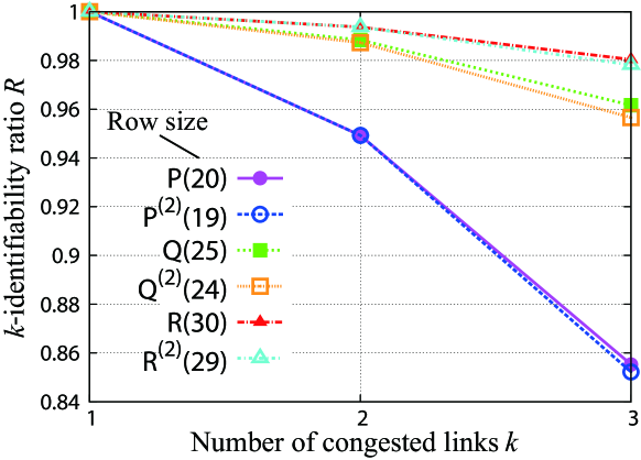
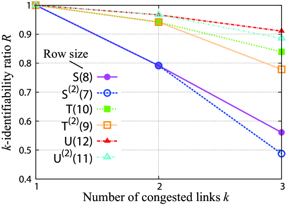
As an implementation of compressed sensing, we employ an $\ell_{1}$-$\ell_{2}$ optimization [7, 8], and evaluate the k-identifiability ratio $R=N^{(k)}/{}_{J}C_{k}$, where $k$ and $N^{(k)}$ denote the number of congested links and the number of the congested link sets which can be identified from the routing matrix and the measurement vector, respectively.

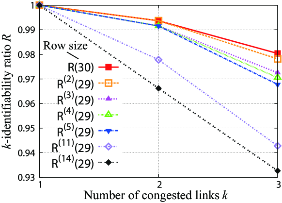
Finally, Table I and II show the tested routing matrices and the differential matrices, respectively. Note that in Table II, the $\ell_{1}$norm of the reference row vector corresponds to the number of links over the selected reference and the reference row is arranged so as to make its order identical to its $\ell_{1}$norm.

Figure 3: k-identifiability ratio $R$ vs. the number of congested links k; dependency on the number of links in the reference path for network topology 1.

Figure 4: k-identifiability ratio $R$ vs. the number of congested links k; effect of the row dimension of routing matrix for network topology $1$.

Figure 5: k-identifiability ratio $R$ vs. the number of congested links k; effect of the dimension of routing matrix for network topology $2$.

V-B Simulation Results

Figs. 3, 4, and 5 show the k-identifiability ratio $R$ vs. the number of congested links k. To evaluate the capacity of the differential routing matrix, it is meaningful to compare its performance with that for its original routing matrix, although the conventional delay tomography scheme does not work at all in the networks where the clock of $s$ is not synchronized to that of $r$. Therefore, for comparison purpose, the three figures contain the performance of the conventional delay tomography scheme when the clock of $s$ is assumed to be synchronized to that of $r$. From Fig. 3, we can see that the shorter path tends to be more acceptable as the reference for the proposed scheme. On the other hand, from Figs. 4 and 5, since the tested matrices have different row sizes which correspond to the number of delay measurements, we can see that the more delay measurements are more advantageous in terms of performance improvement for the proposed and original schemes. For each of given numbers of delay measurements, the proposed scheme, in which a path giving the highest performance is appropriately selected as the reference, performs comparable to the original scheme.

Consequently, in the two networks, because of the clock asynchronism between source and receiver measurement nodes, we have to select a path as the reference in the propose scheme, which leads to a loss of information. However, the information of the reference can be deleted not completely but partially. If an appropriate reference is selected, the differential delay tomography scheme can effectively identify the congested links.

VI Conclusion

In this letter, we proposed a differential delay tomography scheme which enables us to infer link delays without clock synchronization between source and receiver measurement nodes in a network. We theoretically proved that the differential routing matrix preserves the mathematical property of the 1-identifiability of its original routing matrix and evaluated the performance of the proposed scheme by the simulation experiments. Some technical issues remain in the proposed scheme. Particularly, we have to propose an efficient reference selection method. Since the issues are beyond the scope of this letter, we leave them as future works.

We define the r-th row of $\mathbf{d}_{jj^{\prime}}$ and $\mathbf{s}_{jj^{\prime}}$ as $d^{(r)}_{jj^{\prime}}\in\{0,1\}$ and $s^{(r)}_{jj^{\prime}}\in\{0,1\}$, respectively, and the matrices obtained by deleting the r-th row from $\mathbf{d}_{jj^{\prime}}$ and $\mathbf{s}_{jj^{\prime}}$ as $\mathbf{d}^{(-r)}_{jj^{\prime}}$ and $\mathbf{s}^{(-r)}_{jj^{\prime}}$, respectively. Incidentally $\mathbf{A}^{(r)}$ represents the differential matrix of $\mathbf{A}$.
1) If ${\rm dim}(\mathbf{d}_{jj^{\prime}})=I$, that is, $\widetilde{\mathbf{A}}_{jj^{\prime}}=[\mathbf{d}_{jj^{\prime}}~{}~{}\overline{\mathbf{d}}_{jj^{\prime}}]$:

$$\widetilde{\mathbf{A}}^{(r)}_{jj^{\prime}} = [\mathbf{d}^{(-r)}_{jj^{\prime}}-d^{(r)}_{jj^{\prime}}\cdot\mathbf{1}~{}~{}\overline{\mathbf{d}}^{(-r)}_{jj^{\prime}}-\overline{d}^{(r)}_{jj^{\prime}}\cdot\mathbf{1}]$$

$$= \begin{cases}~{}[-\overline{\mathbf{d}}^{(-r)}_{jj^{\prime}}~{}~{}\overline{\mathbf{d}}^{(-r)}_{jj^{\prime}}]&(d^{(r)}_{jj^{\prime}}=1),\\ ~{}[\mathbf{d}^{(-r)}_{jj^{\prime}}~{}~{}-\mathbf{d}^{(-r)}_{jj^{\prime}}]&(d^{(r)}_{jj^{\prime}}=0).\end{cases}$$

Consequently, the two absolute column vectors of $\widetilde{\mathbf{A}}^{(r)}_{jj^{\prime}}$ have no different element, so $\mu(\mathbf{A}^{(r)})=1$.
2) Otherwise:
a) If the r-th row is selected from $\mathbf{d}_{jj^{\prime}}$ then

$$\widetilde{\mathbf{A}}^{(r)}_{jj^{\prime}} = \left[\begin{array}[]{cc}\mathbf{d}^{(-r)}_{jj^{\prime}}-d^{(r)}_{jj^{\prime}}\cdot\mathbf{1}&\overline{\mathbf{d}}^{(-r)}_{jj^{\prime}}-\overline{d}^{(r)}_{jj^{\prime}}\cdot\mathbf{1}\\ \mathbf{s}_{jj^{\prime}}-d^{(r)}_{jj^{\prime}}\cdot\mathbf{1}&\mathbf{s}_{jj^{\prime}}-\overline{d}^{(r)}_{jj^{\prime}}\cdot\mathbf{1}\end{array}\right]$$

$$= \begin{cases}~{}\left[\begin{array}[]{cc}-\overline{\mathbf{d}}^{(-r)}_{jj^{\prime}}&\overline{\mathbf{d}}^{(-r)}_{jj^{\prime}}\\ -\overline{\mathbf{s}}_{jj^{\prime}}&\mathbf{s}_{jj^{\prime}}\end{array}\right]&(d^{(r)}_{jj^{\prime}}=1),\\[15.0pt] ~{}\left[\begin{array}[]{cc}\mathbf{d}^{(-r)}_{jj^{\prime}}&-\mathbf{d}^{(-r)}_{jj^{\prime}}\\ \mathbf{s}_{jj^{\prime}}&-\overline{\mathbf{s}}_{jj^{\prime}}\end{array}\right]&(d^{(r)}_{jj^{\prime}}=0).\end{cases}$$

b) If the r-th row is selected from $\mathbf{s}_{jj^{\prime}}$ then

$$\widetilde{\mathbf{A}}^{(r)}_{jj^{\prime}} = \left[\begin{array}[]{cc}\mathbf{d}_{jj^{\prime}}-s^{(r)}_{jj^{\prime}}\cdot\mathbf{1}&\overline{\mathbf{d}}_{jj^{\prime}}-s^{(r)}_{jj^{\prime}}\cdot\mathbf{1}\\ \mathbf{s}^{(-r)}_{jj^{\prime}}-s^{(r)}_{jj^{\prime}}\cdot\mathbf{1}&\mathbf{s}^{(-r)}_{jj^{\prime}}-s^{(r)}_{jj^{\prime}}\cdot\mathbf{1}\end{array}\right]$$

$$= \begin{cases}~{}\left[\begin{array}[]{cc}-\overline{\mathbf{d}}_{jj^{\prime}}&-\mathbf{d}_{jj^{\prime}}\\ -\overline{\mathbf{s}}^{(-r)}_{jj^{\prime}}&-\overline{\mathbf{s}}^{(-r)}_{jj^{\prime}}\end{array}\right]&(s^{(r)}_{jj^{\prime}}=1),\\[15.0pt] ~{}\left[\begin{array}[]{cc}\mathbf{d}_{jj^{\prime}}&\overline{\mathbf{d}}_{jj^{\prime}}\\ \mathbf{s}^{(-r)}_{jj^{\prime}}&\mathbf{s}^{(-r)}_{jj^{\prime}}\end{array}\right]&(s^{(r)}_{jj^{\prime}}=0).\end{cases}$$

From a) and b), consequently, the two absolute columns of $\widetilde{\mathbf{A}}^{(r)}_{jj^{\prime}}$ still have the different element(s), namely, any two absolute column vectors of $\mathbf{A}^{(r)}$ are still not the same vectors, thus, $\mu(\mathbf{A}^{(r)})<1$.

References

• [1] M. Coates, A. O. Hero III, R. Nowak, and B. Yu, “Internet tomography,” IEEE Signal Process. Mag., vol. 19, no. 3, pp. 47–65, May 2002.
• [2] K. Takemoto, T. Matsuda, and T. Takine, “Sequential Loss Tomography Using Compressed Sensing,” IEICE Trans. Commun., vol. 96, no. 11, pp. 2756-2765, Nov. 2013.
• [3] M. H. Firooz and S. Roy, “Network tomography via compressed sensing,” in Proc. IEEE GLOBECOM 2010, Miami, FL, Dec. 2010.
• [4] W. Xu, E. Mallada, and A. Tang, “Compressive sensing over graphs,” arXiv:1008.0919v1, available: http://arxiv.org/abs/1008.0919, Aug. 2010.
• [5] M.Elad, “Sparse and Redundant Representation,” Springer,2010.
• [6] Y. Xia, and D. Tse, “Inference of link delay in communication networks,” IEEE J. SEL AREAS CCOMMUN., vol. 24, no. 12, pp. 2235–2248, 2006.
• [7] M. Zibulevski and M. Elad, “L1-L2 optimization in signal and image processing,” IEEE Signal Process. Mag., vol. 27, no. 3, pp. 76–88, May. 2010.
• [8] T.Matsuda, M.Nagahara, and K.Hayashi, “Link Quality Classifier with Compressed Sensing Based on 1subscript1\ell_{1}-2subscript2\ell_{2} Optimization,” IEEE Commun Lett., vol. 15, no. 10, pp. 1117–1119, Oct. 2011.