A high-order scheme for solving wave propagation problems via the direct construction of an approximate time-evolution operator

1. Introduction

1.1. Problem formulation

We present a technique for solving a class of linear hyperbolic problems

(1) $$\left\{\begin{aligned} \frac{\partial\mathbf{u}}{\partial t}(\mathbf{x},t)=&\ \mathcal{L}\mathbf{u}(\mathbf{x},t),\qquad&&\mathbf{x}\in\Omega,\quad t>0,\\ \mathbf{u}(\mathbf{x},0)=&\ \mathbf{u}_{0}\left(\mathbf{x}\right)&&\mathbf{x}\in\Omega.\end{aligned}\right.$$

Here $\mathbf{u}$ is a possibly vector valued function and $\mathcal{L}$ is a skew-Hermitian differential operator (see the end of this Section for the method’s scope). The technique is demonstrated on the 2D rotating shallow water equations, as well as the variable coefficient wave equation.

The basic approach is classical, and involves the construction of a rational approximation to the time evolution operator $\exp(\tau\mathcal{L})$ in the form

$$\exp(\tau\mathcal{L})\approx\sum_{m=-M}^{M}b_{m}\,\bigl{(}\tau\mathcal{L}-\alpha_{m}\bigr{)}^{-1},$$

where the time-step $\tau$ is fixed in advance and $M$ scales linearly in $\tau$. Once the time-step $\tau$ has been fixed, an approximate solution at times $\tau,\,2\tau,\,3\tau,\dots$ can be obtained via repeated application of the approximate time-stepping operator, since $\exp(n\tau\mathcal{L})=\bigl{(}\exp(\tau\mathcal{L})\bigr{)}^{n}$. The computational profile of the method is that it takes a moderate amount of work to construct the initial approximation to $\exp(\tau\mathcal{L})$, but once it has been built, it can be applied very rapidly, even for large $\tau$.

The efficiency of the proposed scheme is enabled by (i) a novel method [5] for constructing near optimal rational approximations to oscillatory functions such as $e^{ix}$ over arbitrarily long intervals, and by (ii) the development [17] of a high-order accurate and stable method for pre-computing approximations to operators of the form $(\tau\mathcal{L}-\alpha_{m})^{-1}$. The near optimality of the rational approximations ensures that the number $2M+1$ of terms needed for a given accuracy is typically much smaller than standard methods that rely on polynomial or rational approximations of $\mathcal{L}$.

The proposed scheme has several advantages over typical methods, including the absence of stability constraints on the time step $\tau$ in relation to the spatial discretization, the ability to parallelize in time over many characteristic wavelengths (in addition to any spatial parallelization), and great acceleration when integrating equation (1) for long times or for multiple initial conditions (e.g. when employing an exponential integrator on a nonlinear evolution equation, cf. Section 5). A drawback of the scheme is that it is more memory intensive than standard techniques.

We restrict the scope of this paper to when the application $(\tau\mathcal{L}-\alpha_{m})^{-1}\mathbf{u}_{0}$ can be reduced to the solution of an elliptic-type PDE for one of the unknown variables. This situation arises in geophysical fluid applications (among others), including the rotating primitive equations that are that are used for climate simulations. In this context, the ability to efficiently solve (1) can be used to construct efficient schemes for the fully nonlinear evolution equations in the presence of time scale separation (see [13]). However, the direct solver presented in Section 2 is quite general, and in principle can be extended to first order linear systems of hyperbolic PDEs with little modification (though such an extension is speculative and, in particular, has not been tried).

1.2. Time discretization

In order to time-discretize (1), we fix a time-step $\tau$ (the choice of which is discussed shortly), a requested precision $\delta>0$, and “band-width” $\Lambda\in(0,\infty)$ which specifies the spatial resolution (in effect, the scheme will accurately capture eigenmodes of $\mathcal{L}$ whose eigenvalues $\lambda$ satisfy $|\lambda|\leq\Lambda$). We then use an improved version of the scheme of [5] to construct a rational function,

(2) $$R_{M}(ix)=\sum_{m=-M}^{M}\frac{b_{m}}{\bigl{(}ix-\alpha_{m}\bigr{)}},$$

such that

(3) $$\bigl{|}e^{ix}-R_{M}(ix)\bigr{|}\leq\delta,\qquad x\in[-\tau\Lambda,\tau\Lambda],$$

and

(4) $$|R_{M}(ix)|\leq 1,\qquad x\in\mathbb{R}.$$

It now follows from (3) and (4) that if we approximate $\exp(t\mathcal{L})$ by $R_{M}(\tau\mathcal{L})$, the approximation error satisfies

(5) $$\left\|e^{\tau\mathcal{L}}\mathbf{u}_{0}-\sum_{m=-M}^{M}b_{m}\,\bigl{(}\tau\mathcal{L}-\alpha_{m}\bigr{)}^{-1}\mathbf{u}_{0}\right\|\leq\delta\left\|\mathbf{u}_{0}\right\|+2\left\|\mathbf{u}_{0}-\mathcal{P}_{\Lambda}\mathbf{u}_{0}\right\|,$$

where $\mathcal{P}_{\Lambda}$ projects functions onto the subspace spanned by eigenvectors of $\mathcal{L}$ with modulus at most $\Lambda$. Here the only property of $\mathcal{L}$ that we use is that $\mathcal{L}$ is skew-Hermitian, and hence has a complete spectral decomposition with a purely imaginary spectrum.

The bound (4) ensures that the repeated application of $R_{M}(\tau\mathcal{L})$ is stable on the entire imaginary axis. It also turns out that the number $2M+1$ of terms needed in the rational approximation in (3) is close to optimally small (for the given accuracy $\delta$).

The scheme described above allows a great deal of freedom in the choice of the time step $\tau$. While classical methods typically require the time step to be a small fraction of the characteristic wavelength, we have freedom to let $\tau$ cover a large number of characteristic wavelengths. Therefore, the scheme is well suited to parallelization in time, since all the inverse operators in the approximation of the operator exponential can be applied independently. In fact, the only constraint on the size of $\tau$ is on the memory available to store the representations of the inverse operators (as explained in Section 1.3, the memory required for each inverse scales linearly in the number of spatial discretization parameters, up to a logarithmic factor).

1.3. Pre-computation of rational functions of $\mathcal{L}$

The time discretization technique described in Section 1.2 requires us to build explicit approximations to differential operators on the domain $\Omega$ such as $(\tau\mathcal{L}-\alpha_{m})^{-1}$. We do this using a variation of the technique described in [17]. A variety of different domains can be handled, but for simplicity, suppose that $\Omega$ is a rectangle. The idea is to tessellate $\Omega$ into a collection of smaller rectangles, and to put down a tensor product grid of Chebyshev nodes on each rectangle, as shown in Figure 1. A function is represented via tabulation on the nodes, and then $\mathcal{L}$ is discretized via standard spectral collocation techniques on each patch. The patches are glued together by enforcing continuity of both function values and normal derivatives. This discretization results in a block sparse coefficient matrix, which can rapidly be inverted via a procedure very similar to the classical nested dissection technique of George [9]. The resulting inverse is dense but “data-sparse,” which is to say that it has internal structure that allows us to store and apply it efficiently.

In order to describe the computational cost of the direct solver, let $N$ denote the number of nodes in the spatial discretization. For a problem in two dimensions, the “build stage” of the proposed scheme constructs $2M+1$ data-sparse matrices $\{\bm{\mathsf{A}}_{m}\}_{m=-M}^{M}$ of size $N\times N$, where each $\bm{\mathsf{A}}_{m}$ approximates $(\tau\mathcal{L}-\alpha_{m})^{-1}$. The build stage has asymptotic cost $\mathcal{O}(M\,N^{1.5})$, and storing the matrices requires $O(M\,N\,\log(N))$ memory. The cost of applying a matrix $\bm{\mathsf{A}}_{m}$ is $\mathcal{O}(N\,\log\left(N\right))$. (We remark that the cost of building the matrices $\{\bm{\mathsf{A}}_{m}\}_{m=-M}^{M}$ can often be accelerated to optimal $\mathcal{O}(M\,N)$ complexity [10], but since the pre-factor in the $\mathcal{O}(M\,N^{1.5})$ bound is quite small, such acceleration would have negligible benefit for the problem sizes under consideration here.) Section 2 describes the inversion procedure in more detail.

We remark that the spatial discretization procedure we use does not explicitly enforce that the discrete operator is exactly skew-Hermitian. However, the fact that the spatial discretization is done to very high accuracy means that it is in practice very nearly so. Numerical experiments indicate that the scheme as a whole is stable in every regime where it was tested.

1.4. Comparison to existing approaches

The approach of using proper rational approximations for applying matrix exponentials has a long history. In the context of operators with negative spectrum (e.g. for parabolic-type PDEs), many authors have discussed how to compute efficient rational approximations to the decaying exponential $e^{-x}$, including using Cauchy’s integral formula coupled with Talbot quadrature (cf. [23]), and optimal rational approximations via the Carathéodory-Fejer method (cf. [23]) or the Remez algorithm [3]. However, such methods are less effective (or not applicable) when applied to approximating oscillatory functions such as $e^{ix}$ over long intervals. For computing functions of parabolic-type linear operators, the approach of combining rational approximations and compressed representations of the solution operators using so-called $\mathcal{H}$-matrices has been proposed in [8].

Common approaches for applying the exponential of skew-Hermitian operators include high-order time-stepping methods, scaling-and-squaring coupled with Padé approximations (cf. [14]) or Chebyshev polynomials (cf. [1]), and polynomial or rational Krylov methods (cf. [15] and [11]). All these methods iteratively build up rational or polynomial approximations to the operator exponential, and correspondingly approximate the spectrum $e^{i\omega_{n}\tau}$ of $e^{\tau\mathcal{L}}$ with polynomials or rationals. Therefore, the near optimality of (2) and the speed of applying the inverse operators in (5) will generally translate into high efficiency relative to standard methods. In contrast to these standard approaches, the method proposed in this paper can also be trivially parallelized in time over many characteristic wavelengths.

In addition to approaches that rely on polynomial or rational approximations, let us mention two alternative approaches for time-stepping on wave propagation problems. The authors in [2] combine separated representations of multi-dimensional operators, partitioned low rank compressions of matrices, and (near) optimal quadrature nodes for band-limited functions, in order to compute compressed representations of the operator exponential over $1-2$ characteristic wavelengths. Along different lines, the authors in [6] use wave atoms to construct compressed representations of the (short time) operator exponential, and in particular can bypass the CFL constraint.

1.5. Outline of manuscript

The paper is organized as follows. In Section 2, we briefly describe the direct solver in [17]. We then discuss in Section 3 a technique for constructing efficient rational approximations of general functions, and specialize to the case of approximating the exponential $e^{ix}$ and the phi-functions for exponential integrators [4]. In Section 4, we present applications of the method for both the 2D rotating shallow water equations and the 2D wave equation in inhomogenous medium. In particular, we compare the accuracy and efficiency of this approach against $4$th order Runge-Kutta and the Chebyshev polynomial method (in our comparisons, we use the same spectral element discretization). Finally, Appendix A contains error bounds for the rational approximations constructed here.

2. Spectral element discretization

This section describes how to efficiently compute a highly accurate approximation to the inverse operator $\left(\mathcal{L}-\alpha\right)^{-1}$, where $\mathcal{L}$ is a skew-Hermitian operator. As mentioned in the introduction, we restrict our discussion to environments where application of the inverse can be reformulated as a scalar elliptic problem. This reformulation procedure is illustrated for the classical wave equation and for the shallow water equations in Section 2.1. Section 2.2 describes a high-order multidomain spectral discretization procedure for the elliptic equation. Section 2.3 describes a direct solver for the system of linear equations arising upon discretization.

2.1. Reformulation as an elliptic problem

In many situations of practical interest, the task of solving a hyperbolic equation $(\mathcal{L}-\alpha)u=f$, where $\mathcal{L}$ is a skew-Hermitian operator, can be reformulated as an associated elliptic problem. In this section, we illustrate the idea via two representative examples. Example $1$ is of particular relevance to geophysical fluid applications, which serve as a major motivation of this algorithm.

Example 1 — the shallow water equation: We consider the rotating shallow water equations,

(6) $$\mathbf{v}_{t} = -fJ\mathbf{v}+\nabla\eta,$$

$$\eta_{t} = \nabla\cdot\mathbf{v},$$

where $\mathbf{v}\left(\mathbf{x}\right)=\left(v_{1}\left(\mathbf{x}\right),v_{2}\left(\mathbf{x}\right)\right)$ denotes the fluid velocity, $\eta\left(\mathbf{x}\right)$ denotes perturbed surface elevation, $f$ is the (possibly spatially varying) Coriolis frequency, and

$$J=\left(\begin{array}[]{cc}0&1\\ -1&0\end{array}\right).$$

On the sphere, $f=2\Omega\sin\phi$; on the plane, $f$ is constant. We write system (6) in the form

$$\mathbf{u}_{t}=\mathcal{L}\mathbf{u},$$

where

(7) $$\mathcal{L}\left(\begin{array}[]{c}\mathbf{v}\\ \eta\end{array}\right)=\left(\begin{array}[]{c}-fJ\mathbf{v}+\nabla\eta\\ \nabla\cdot\mathbf{v}\end{array}\right).$$

Although we only consider the case when the Coriolis frequency is constant, the method generalizes to non-constant coefficient $f$ (see also the example in the next section) and is of particular relevance for a spectral element discretization on the cubed sphere.

In order to apply the method in this paper, we use the standard fact (cf. [22]) that if

(8) $$\left(\mathcal{L}-\alpha\right)\left(\begin{array}[]{c}\mathbf{v}\\ \eta\end{array}\right)=\left(\begin{array}[]{c}\mathbf{v_{0}}\\ \eta_{0}\end{array}\right),$$

then $\eta$ satisfies the elliptic equation

(9) $$\nabla\cdot\left(\mathcal{A}_{\alpha}\nabla\eta\right)-\alpha\eta=\eta_{0}+H\nabla\cdot\mathcal{A}_{\alpha}\mathbf{v_{0}}.$$

Here $\mathcal{A}_{\alpha}$ is defined by

$$\mathcal{A}_{\alpha}=\frac{1}{\alpha^{2}+f^{2}}\left(\begin{array}[]{cc}\alpha&f\\ -f&\alpha\end{array}\right).$$

Once $\eta$ is computed, $\mathbf{v}$ can be obtained directly,

(10) $$\mathbf{v}=-\mathcal{A}_{\alpha}\mathbf{v_{0}}+\mathcal{A}_{\alpha}\nabla\eta.$$

When $f$ is constant, equation (9) reduces to

(11) $$\left(\Delta-\frac{\alpha^{2}+f^{2}}{c^{2}}\right)\eta=\frac{\alpha^{2}+f^{2}}{c^{2}\alpha}\left(\eta_{0}+H\nabla\cdot\left(\mathcal{A}_{\alpha}\mathbf{v_{0}}\right)\right).$$

Example 2 — the wave equation: Consider the wave propagation problem

(12) $$u_{tt}=\kappa\Delta u,\,\,\,\,\mathbf{x}\in\left[0,1\right]\times\left[0,1\right],$$

where $\kappa\left(\mathbf{x}\right)>0$ is a smooth function, the initial conditions $u\left(\mathbf{x},0\right)$ and $u_{t}\left(\mathbf{x},0\right)$ are prescribed, and periodic boundary conditions are used.

In order to apply the method in this paper, we reformulate (32) as a first order system in both time and space by defining $v=u_{t}$, $w=u_{x}$, and $z=u_{y}$. Then we have that

(13) $$\left(\begin{array}[]{c}w_{t}\\ z_{t}\\ v_{t}\end{array}\right)=\left(\begin{array}[]{ccc}0&0&\partial_{x}\\ 0&0&\partial_{y}\\ \kappa\partial_{x}&\kappa\partial_{y}&0\end{array}\right)\left(\begin{array}[]{c}w\\ z\\ v\end{array}\right),$$

with initial conditions

$$v\left(\mathbf{x},0\right)=u_{0}\left(\mathbf{x}\right),\,\,\,w\left(\mathbf{x},0\right)=\frac{\partial u_{0}}{\partial x}\left(\mathbf{x}\right),\,\,\,z\left(\mathbf{x},0\right)=\frac{\partial u_{0}}{\partial y}\left(\mathbf{x}\right).$$

Here the scalar function $u$ to the original system (32) can be recovered after the final time step by solving the elliptic equation $\Delta u=w_{x}+z_{y}$.

To apply the method in this paper, we compute the solution to

(14) $$\left(\mathcal{L}-\alpha\right)\left(\begin{array}[]{c}w\\ z\\ v\end{array}\right)=\left(\begin{array}[]{c}v_{x}-\alpha w\\ v_{y}-\alpha z\\ \kappa\left(w_{x}+z_{y}\right)-\alpha v\end{array}\right)=\left(\begin{array}[]{c}w_{0}\\ z_{0}\\ v_{0}\end{array}\right)$$

as follows. First, solving for $w$ and $z$ in terms of $v$,

(15) $$w=\frac{1}{\alpha}\left(v_{x}-w_{0}\right),\,\,\,\,z=\frac{1}{\alpha}\left(v_{y}-z_{0}\right),$$

it is straightfoward to show that

(16) $$\left(\Delta-\alpha^{2}\kappa^{-1}\right)v=\alpha\kappa^{-1}v_{0}+\frac{\partial w_{0}}{\partial x}+\frac{\partial z_{0}}{\partial y}.$$

Once $v$ is known, $w$ and $z$ can then be computed directly via (15).

2.2. Discretization

In this section, we describe a high-order accurate discretization scheme for elliptic boundary value problems such as (11) and (16) which arise in the solution of hyperbolic evolution equations. Specifically, we describe the solver for a boundary value problem (BVP) of the form

(17) $$\mathcal{B}u\left(\mathbf{x}\right)=f\left(\mathbf{x}\right),\,\,\,\mathbf{x}\in\Omega,$$

where $\mathcal{B}$ is an elliptic differential operator. To keep things simple, we consider only square domains $\Omega=[0,1]^{2}$, but the solver can easily be generalized to other domains. The solver we use is described in detail in [18], our aim here is merely to give a high-level conceptual description.

The PDE (17) is discretized using a multidomain spectral collocation method. Specifically, we split the square $\Omega$ into a large number of smaller squares (or rectangles), and then put down a tensor product grid of $p\times p$ Chebyshev nodes on each small square, see Figure 1. The parameter $p$ is chosen so that dense computations involving matrices of size $p^{2}\times p^{2}$ are cheap ($p=20$ is often a good choice). Let $\{\mathbf{x}_{j}\}_{j=1}^{N}$ denote the total set of nodes. Our approximation to the solution $u$ of (17) is then represented by a vector $\mathbf{u}\in\mathbb{C}^{N}$, where the $j$’th entry is simply an approximation to the function value at node $\mathbf{x}_{j}$, so that $\mathbf{u}(j)\approx u(\mathbf{x}_{j})$. The discrete approximation to (17) then takes the form

(18) $$\mathbf{B}\mathbf{u}=\mathbf{f},$$

where $\mathbf{B}$ is an $N\times N$ matrix. The $j$’th row of (18) is associated with a collocation condition for node $\mathbf{x}_{j}$. For all $j$ for which $\mathbf{x}_{j}$ is a node in the interior of a small square (filled circles in Figure 1), we directly enforce (17) by replacing all differentiation operators by spectral differentiation operators on the local $p\times p$ tensor product grid. For all $j$ for which $\mathbf{x}_{j}$ lies on a boundary between two squares (hollow squares in Figure 1), we enforce that normal fluxes across the boundary are continuous, where the fluxes from each side of the boundary are evaluated via spectral differentiation on the two patches (corner nodes need special treatment, see [18]).

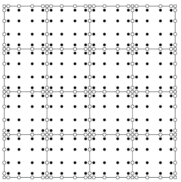
Figure 1. Illustration of the grid of points $\{\mathbf{x}_{j}\}_{j=1}^{N}$ introduced to discretize (17) in Section 2.2. The figure shows a simplified case involving $4\times 4$ squares, each holding a $6\times 6$ local tensor product grid of Chebyshev nodes. The PDE (17) is enforced via collocation using spectral differentiation on each small square at all solid (“internal”) nodes. At the hollow (“boundary”) nodes, continuity of normal fluxes is enforced.

2.3. Direct solver

The discrete linear system (18) arising from discretization of (17) is block-sparse. Since it has the typical sparsity pattern of a matrix discretizing a 2D differential operator, it is possible to compute its LU factorization in $O(N^{1.5})$ operations using a nested dissection ordering of the nodes [7, 9] that minimizes fill-in. Once the LU-factors have been computed, the cost of a linear solve is $O(N\log N)$. In the numerical computations presented in Section 4, we use a slight variation of the nested-dissection algorithm that was introduced in [17] for the case of homogeneous equations. The extension to the situation involving body loads is straight-forward, see [18].

We note that by exploiting internal structure in the dense sub-matrices that appear in the factors of $\mathbf{B}$ as the factorization proceeds, the complexity of both the factorization and the solve stages can often be reduced to optimal $O(N)$ complexity [10]. However, for the problem sizes considered in this manuscript, there would be little practical gain to implementing this more complex algorithm.

3. constructing rational approximations

We now discuss how to construct efficient rational approximations to general smooth functions $f\left(x\right)$. For concreteness, we consider approximating the phi functions

$$\varphi_{0}\left(x\right)=e^{ix},\,\,\,\varphi_{1}\left(x\right)=\frac{e^{ix}-1}{ix},\,\,\,\varphi_{2}\left(x\right)=\frac{e^{ix}-ix-1}{ix^{2}},$$

that arise for high-order exponential integrators (cf. [23]). By considering the real and imaginary components separately, we assume that $f\left(x\right)$ is real-valued (it turns out that the poles in the approximation will be the same for the real and imaginary components).

The construction proceeds in two steps; the second step is actually a pre-computation and need only be done once, but is presented last for clarity. First, we construct an approximation to $f\left(x\right)$ by sums of shifted Gaussians $\psi_{h}\left(x\right)=\left(4\pi\right)^{-1/2}e^{-x^{2}/\left(4h^{2}\right)}$ (see Section 3.1 for details),

(19) $$\left|f\left(x\right)-\sum_{-M}^{M}b_{m}\psi_{h}\left(x+nh\right)\right|\leq\delta_{1},\,\,\,\,-\Lambda\leq x\leq\Lambda.$$

Here $h$ is inversely proportional to the bandlimit of $f\left(x\right)$, and $M$ controls the interval $\Lambda$ over which the approximation is valid (roughly $\left|x\right|\lesssim Mh$). When $f\left(x\right)=e^{ix}$, the coefficients are explicitly given by $c_{m}=\left(\widehat{\psi_{h}}\left(1\right)/h\right)e^{-2\pi inh}$, and the approximation is remarkably accurate (see 23 for error bounds). Second, using the approach in [5], a rational approximation to $\psi_{1}\left(x\right)=\left(4\pi\right)^{-1/2}e^{-x^{2}/4}$ is constructed over the real line (see Section 3.2 for details),

(20) $$\left|\psi_{1}\left(x\right)-2\text{Re}\left(\sum_{j=-L}^{L}\frac{a_{j}}{ix-\left(\mu+ij\right)}\right)\right|\leq\delta_{2},\,\,\,\,x\in\mathbb{R}.$$

Notice that the imaginary parts of the poles in the above approximation are integer multiples $j=0,\pm 1,\ldots,\pm L$. For $L=11$, we construct $\mu$ and coefficients $a_{j}$ such that the $L^{\infty}$ approximation error $\delta_{2}$ satisfies $\delta_{2}<10^{-12}$ (see Table 1). Finally, combining (19) and (20), we obtain a rational approximation to $f\left(x\right)$,

$$\left|f\left(x\right)-2\text{Re}\left(\sum_{n=-M-L}^{M+L}\frac{c_{n}}{ix-h\left(\mu+in\right)}\right)\right|\leq\delta_{1}+2\left(M+L\right)\delta_{2}.$$

Here the coefficients $c_{n}$ are given by

$$c_{n}=h\sum_{k=L_{1}}^{L_{2}}a_{k}b_{n-k},$$

where

$$L_{1}\left(n\right)=\max\left(-L,n-M\right),\,\,\,\,L_{2}\left(n\right)=\max\left(-L,n-M\right).$$

Importantly, constructing the rational approximation (20) to $\psi\left(x\right)$ need only be done once. In particular, once $\mu$ and the coefficients $a_{j}$ are pre-computed, rational approximations to general functions $f\left(x\right)$ over arbitrarily long spatial intervals can be obtained with minimal effort, as discussed in Section 3.1. We present $\mu$, and the coefficients $a_{j}$, $j=-11,\ldots,11$, in Table 1, which are sufficient to yield an $L^{\infty}$ error $\delta_{1}\approx 7\times 10^{-13}$ in (20) .

Using the reduction algorithm in [12], we find that the rational approximation constructed for $e^{ix}$ is close to optimal in the $L^{\infty}$ norm, for a given accuracy $\delta$ and spatial cutoff $A$. In fact, the construction in this paper uses only $1.2$ times more poles than the near optimal rational approximation obtained from [12] (when $\delta=10^{-10}$ and $A=56\pi$, which we use in our numerical experiments). We note that the residues corresponding to this near optimal approximation can be very large and, for this reason, we prefer to use the sub-optimal approximation instead.

As clarified in Sections 3.1 and 3.2, the same poles can be used to approximate multiple functions with the same bandlimit. For example, we can use the same poles to approximate all functions $e^{2\pi itx}$, for $0\leq t\leq 1$, since all these functions have bandlimit less than or equal to $e^{2\pi ix}$; the dependence on $t$ is only through the coefficients, which are given explicitly by $c_{m}=\left(\widehat{\psi_{h}}\left(t\right)/h\right)e^{-2\pi inth}$. In particular, the poles $\alpha_{m}=h\left(\mu+im\right)$ are independent of $t$ and yield uniformly accurate approximations to $e^{itx}$ on the same interval $\left[-\Lambda,\Lambda\right]$. This observation enables the efficient computation of multiple operator exponentials $e^{s_{k}\mathcal{L}}\mathbf{u}_{0}$, for $s_{k}=tk/L$, using the same computed solutions $\left(t\mathcal{L}-\alpha_{m}\right)^{-1}\mathbf{u}_{0}$, $m=1,\ldots,M$. A similar comment applies to the phi-functions from exponential integrators.

Generally, any rational approximation to $e^{ix}$ (or more general functions) must share the same number of zeros within the interval of interest; in particular, since the rational approximation can be expressed as a quotient of polynomials, it is therefore subject to the Nyquist constraint. However, one advantage of this approximation method is that it allows efficient rational approximations of functions that are spatially localized. In fact, since the approximation (19) involves highly localized Gaussians, the subsequent rational approximations are able to represent spatially localized functions as well as highly oscillatory functions using (perhaps a subset) of the same collection of poles. This allows the ability to take advantage of spectral gaps (e.g. from scale separation between fast and slow waves) and possibly bypass the Nyquist constraint under certain circumstances.

3.1. Gaussian approximations to a general function

We discuss how to construct the approximation (19). To do so, we choose $h$ small enough that the function $\hat{f}\left(\xi\right)$ is zero (or approximately so) outside the interval $\left[-1/\left(2h\right),1/\left(2h\right)\right]$. Then we can expand $\hat{f}\left(\xi\right)/\widehat{\psi_{h}}\left(\xi\right)$ in a Fourier series,

(21) $$\frac{\hat{f}\left(\xi\right)}{\widehat{\psi_{h}}\left(\xi\right)}=\sum_{-\infty}^{\infty}c_{m}e^{2\pi imh\xi},$$

where

$$c_{m}=h\int_{-1/\left(2h\right)}^{1/\left(2h\right)}e^{-2\pi imh\xi}\frac{\hat{f}\left(\xi\right)}{\widehat{\psi_{h}}\left(\xi\right)}d\xi.$$

Transforming (21) back to the spatial domain, we have that

$$f\left(x\right)=\sum_{-\infty}^{\infty}c_{m}\psi_{h}\left(x+mh\right).$$

Notice that the functions $\psi_{h}\left(x+mh\right)$ are tighly localized in space, and truncating the above series from $-M$ to $M$ yields accurate approximations for $-\left(M-b\right)hx<x<\left(M-b\right)hx$, where $b>0$ is a small number that is related to the decay of $\psi_{h}\left(x\right)$. We remark that the authors in [19] discuss a related method of constructing quasi-interpolating representations via sums of Gaussians (see [20] for a comprehensive survey).

Specializing to the case when $f\left(x\right)=e^{2\pi ix}$, we have that $\hat{f}\left(\xi\right)=\delta\left(\xi-1\right)$, and so the coefficients $c_{m}$ are given by

(22) $$c_{m}=\frac{h}{\widehat{\psi_{h}}\left(1\right)}e^{-2\pi imh}.$$

Similarly, for functions $\varphi_{1}\left(x\right)$ and $\varphi_{2}\left(x\right)$, the coefficients $c_{m}$ can be obtained numerically using the fact that

$$\widehat{\phi_{1}}\left(\xi\right)=\begin{cases}2\pi,&\,\,\,\,-\frac{1}{2\pi}\leq\xi\leq 0,\\ 0,&\,\,\,\,\text{otherwise.}\end{cases}$$

and

$$\widehat{\phi_{2}}\left(\xi\right)=\begin{cases}\left(2\pi\right)^{2}\left(\xi+\frac{1}{2\pi}\right),&\,\,\,\,-\frac{1}{2\pi}\leq\xi\leq 0,\\ 0,&\,\,\,\,\text{otherwise.}\end{cases}$$

For example, the coefficients $c_{m}$ for e.g. $\phi_{1}\left(x\right)$ can be computed via discretization of the integral,

$$c_{m}=h\int_{-1/\left(2\pi\right)}^{0}e^{-2\pi imh\xi}\frac{e^{-2\pi imh\xi}}{\widehat{\psi_{h}}\left(\xi\right)}d\xi.$$

Figure 2. The absolute error in the Gaussian approximations of $\varphi_{j}\left(x\right)$ for $j=1,2$ (plots (a) and (b)) , using $h=1$ and $M=200$.

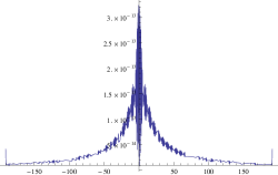
(a)        (a)    

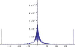
In Figure 2, we plot the error,

$$\left|\varphi_{j}\left(x\right)-\sum_{-\infty}^{\infty}c_{m,j}\psi\left(x+mh\right)\right|,$$

for the phi functions $\varphi_{1}\left(x\right)$ and $\varphi_{1}\left(x\right)$, where we choose $h=1$ and $M=200$; notice that the choice of $h$ corresponds to the bandlimit of $\varphi_{j}\left(x\right)$. As shown in Figure 2, the error is smaller than $\approx 3\times 10^{-13}$ for all $-191\leq x\leq 191$, and is shown to begin to rise at the ends of the intervals, which are close to $Mh$. This behavior can be understood by noting that

$$\left|\varphi_{j}\left(x\right)-\sum_{-M}^{M}c_{m,j}\psi_{1}\left(x+m\right)\right|\leq\sum_{\left|m\right|>M}\left|c_{m,j}\right|\psi_{1}\left(x+m\right),$$

where we used that the support of $\widehat{\varphi_{j}}$ is contained in $\left[-1/2,1.2\right]$. Since the functions $\psi_{1}\left(x+m\right)$ for $m>M$ decay rapidly away from $x=-m$, the error from truncation is negligible when $\left|x\right|\leq\left(M-m_{0}\right)$ and $m_{0}=\mathcal{O}\left(1\right)$.

We remark that, for the function $e^{ix}$, it can be shown (see the Appendix) that the approximation for $e^{ix}$ satisfies

(23) $$\left|e^{ix}-\sum_{m=-M}^{M}c_{m}\psi_{h}\left(x+mh\right)\right|\leq\frac{1}{\widehat{\psi_{h}}\left(1\right)}\left(\sum_{k\neq 0}\widehat{\psi_{h}}\left(\frac{k}{h}\right)+\sum_{\left|m\right|>M}\psi_{h}\left(x+mh\right)\right),$$

where $c_{m}$ is defined in (22). We see that the first sum is negligible for e.g. $h\lesssim 1$, owing to the tight frequency localization of $\psi_{h}$. Similarly, the second sum is negligible when $\left|x\right|\leq\left(M-m_{0}\right)h$ and $m_{0}=\mathcal{O}\left(1\right)$, owing to the tight spatial localization of $\psi$.

3.2. Rational approximation to a Gaussian

We now discuss how to construct the approximation (20).

To do so, we first use AAK theory (see [5] for details) to construct a near optimal rational approximation,

$$\left|\frac{1}{\sqrt{4\pi}}e^{-x^{2}/4}-\text{Re}\left(\sum_{j=1}^{N}\frac{b_{j}}{ix+\alpha_{j}}\right)\right|\leq\delta.$$

For an accuracy of $\delta\approx 10^{-13}$, $13$ poles $\gamma_{j}$ are required.

Setting $\mu=\min_{j}\text{Re}\left(\alpha_{j}\right)$ , we next look for a rational approximation to $\left(4\pi\right)^{-1/2}e^{-x^{2}/4}$ of the form

(24) $$R\left(x\right)=\text{Re}\left(\sum_{j=-L}^{L}\frac{a_{j}}{ix+\mu+ij}\right),$$

where we take $L=11$. We find the coefficients $a_{j}$ by minimizing the $L^{\infty}$ error

$$\left\|\frac{1}{\sqrt{4\pi}}e^{-x^{2}/4}-\text{Re}\left(\sum_{j=-L}^{L}\frac{a_{j}}{ix_{n}+\mu+ij}\right)\right\|_{\infty},$$

where the points $x_{n}\in\left[-30,30\right]$ are chosen to be more sparsely distributed outside the numerical support of $e^{-x^{2}/4}$; the interval $\left[-30,30\right]$ is found experimentally to yield high accuracy for the approximation over the entire real line. Finding the coefficients $a_{j}$, $j=-L,\ldots,L$, that minimize the $L^{\infty}$ error can be cast as a convex optimization problem, and a standard algorithm can be used (we use Mathematica). The resulting approximation error is shown in Figure 3; the error remains less than $\approx 7\times 10^{-13}$ for all $x\in\mathbb{R}$.

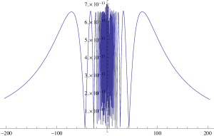
Figure 3. Error in the rational approximation (20) to $e^{-x^{2}/4}$

We display the real number $\mu$, and the coefficients $a_{j}$, $j=1,\ldots,11$. In particular, these numbers are the only parameters that are needed in order to construct rational approximations to general functions on spatial intervals of any size.

Table 1. Coefficients $a_{j}$, $j=-11,\ldots,11$, and number $\mu$, in the rational approximation (24).

$\mu=-4.315321510875024$,

$a_{-11}=\left(-1.0845749544592896\times 10^{-7},2.77075431662228\times 10^{-8}\right)$,

$a_{-10}=\left(1.858753344202957\times 10^{-8},-9.105375434750162\times 10^{-7}\right)$,

$a_{-9}=\left(3.6743713227243024\times 10^{-6},7.073284346322969\times 10^{-7}\right)$,

$a_{-8}=\left(-2.7990058083347696\times 10^{-6},0.0000112564827639346\right)$,

$a_{-7}=\left(0.000014918577548849352,-0.0000316278486761932\right)$,

$a_{-6}=\left(-0.0010751767283285608,-0.00047282220513073084\right)$,

$a_{-5}=\left(0.003816465653840016,0.017839810396560574\right)$,

$a_{-4}=\left(0.12124105653274578,-0.12327042473830248\right)$,

$a_{-3}=\left(-0.9774980792734348,-0.1877130220537587\right)$,

$a_{-2}=\left(1.3432866123333178,3.2034715228495942\right)$,

$a_{-1}=\left(4.072408546157305,-6.123755543580666\right)$,

$a_{0}=-9.442699917778205$,

$a_{1}=\left(4.072408620272648,6.123755841848161\right)$,

$a_{2}=\left(1.3432860877712938,-3.2034712658530275\right)$,

$a_{3}=\left(-0.9774985292598916,0.18771238018072134\right)$,

$a_{4}=\left(0.1212417070363373,0.12326987628935386\right)$,

$a_{5}=\left(0.0038169724770333343,-0.017839242222443888\right)$,

$a_{6}=\left(-0.0010756025812659208,0.0004731874917343858\right)$,

$a_{7}=\left(0.000014713754789095218,0.000031358475831136815\right)$,

$a_{8}=\left(-2.659323898804944\times 10^{-6},-0.000011341571201752273\right)$,

$a_{9}=\left(3.6970377676364553\times 10^{-6},-6.517457477594937\times 10^{-7}\right)$,

$a_{10}=\left(3.883933649142257\times 10^{-9},9.128496023863376\times 10^{-7}\right)$,

$a_{11}=\left(-1.0816457995911385\times 10^{-7},-2.954309729192276\times 10^{-8}\right)$

In Figure 4, we show the resulting rational approximations of $\cos\left(2\pi x\right)$ and $\sin\left(2\pi x\right)$, which use the same $172$ complex-conjugate pairs of poles; the $L^{\infty}$ error is seen to be $\approx 10^{-10}$ over the interval $-28\leq x\leq 28$.

Figure 4. Error in the rational approximations of $\sin\left(2\pi x\right)$ and $\cos\left(2\pi x\right)$ (plots (a) and (b)), for $-28\leq x\leq 28$. These approximations use the same $172$ pairs of complex-conjugate poles.

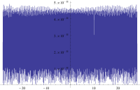
(a)         (b)    

3.3. Constructing rational approximation of modulus bounded by unity

Figure 5. (a) Plot of the rational filter function $S\left(ix\right)$, for $-60\leq x\leq 60$.   (b) Plot of the difference $\left|S\left(ix\right)-1\right|$ for $-28\leq x\leq 28$.

(a)                                      (b)

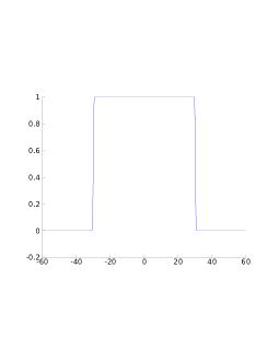
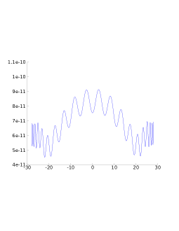
For our applications, it is important that the approximation to $e^{ix}$ is bounded by unity on the real line. In particular, the Gaussian approximation for $e^{ix}$ constructed in Section 3.1 has absolute value larger than one when $\left|x\right|\approx Mh$, and this can lead to instability in repeated applications of $e^{t\mathcal{L}}$.

The basic idea is to construct a rational function $S\left(ix\right)$ that satisfies $S\left(ix\right)\approx 1$ for $\left|x\right|\lesssim M_{0}h$ and $S\left(ix\right)\approx 0$ for $\left|x\right|\gtrsim M_{0}h$. As long as $M_{0}$ is slightly less than $M$, the function $S\left(ix\right)R_{M}\left(ix\right)$ accurately approximates $e^{ix}$ for $\left|x\right|\lesssim M_{0}h$, and decays rapidly to zero for $\left|x\right|\gtrsim M_{0}h$. Therefore, $\left|S\left(ix\right)R_{M}\left(ix\right)\right|\leq 1$ for all $x\in\mathbb{R}$, and repeated application of $S\left(t\mathcal{L}\right)R_{M}\left(t\mathcal{L}\right)\mathbf{u}_{0}$ is stable for all $t>0$. In Figure 5, we plot rational filter that uses $33$ complex-conjugate poles; we see that $\left|S\left(ix\right)-1\right|\approx 10^{-10}$ for $-28\leq x\leq 28$.

Although the above approach results in a stable method, we have found it more efficient to use a slightly modified version. This is motivated by the following simple observation: since $\mathbf{u}_{0}\left(\mathbf{x}\right)$ is real-valued,

(25) $$\overline{\left(t\mathcal{L}-\alpha\right)^{-1}\mathbf{u}_{0}}=\left(t\mathcal{L}-\overline{\alpha}\right)^{-1}\mathbf{u}_{0}.$$

Recalling that the poles from Section 3.2 come in complex-conjugate pairs, only half the matrix inverses need to be pre-computed and applied if (25) is used. However, directly using (25) results in numerical instabilities, where small errors in the high frequencies are amplified after successive applications of $R_{M}\left(t\mathcal{L}\right)\mathbf{u}_{0}$. The fix is to eliminate the errors in the high frequency components by instead computing $S\left(k_{0}\Delta\right)R_{M}\left(t\mathcal{L}\right)\mathbf{u}_{0}$, where $k_{0}$ is determined by the frequency content of $\mathbf{u}_{0}\left(\mathbf{x}\right)$ and the operator $S\left(k_{0}\Delta\right)$ only affects the highest wavenumbers. Since the transition region between $S\left(ix\right)\approx 1$ and $S\left(ix\right)\approx 0$ can be made arbitrarily small (see Figure 5), the operator $S\left(k_{0}\Delta\right)$ behaves like a spectral projector.

We now discuss how to construct $S\left(ix\right)$. To do so, we use that (see [21])

$$\left|\frac{1}{\widehat{\psi_{h}}\left(1\right)}\sum_{-\infty}^{\infty}\psi_{h}\left(x+hm\right)-1\right|\leq\frac{1}{h\widehat{\psi_{h}}\left(1\right)}\sum_{k\neq 0}\widehat{\psi_{h}}\left(\frac{k}{h}\right),$$

which follows from the Poisson summation formula. For $h\lesssim 1$, the right hand side is negligible, owing to the tight frequency localization of $\widehat{\psi_{h}}\left(\xi\right)$. Truncating the above sum and using the tight spatial localiztion of $\psi_{h}\left(x\right)$, we see that the function

(26) $$\chi\left(x\right)=\sum_{-M_{0}}^{M_{0}}\psi_{h}\left(x+mh\right),$$

is approximately unity for $\left|x\right|\lesssim M_{0}h$, and decays to zero rapidly when $\left|x\right|\gtrsim M_{0}h$. It also holds out that $\left|\chi\left(x\right)\right|\leq 1$ for all $x\in\mathbb{R}$. Therefore, using the techniques from Sections 3.1 and 3.2, we construct a rational approximation $Q\left(ix\right)$ to the function $\chi\left(x\right)$ in (26),

(27) $$\left|Q\left(ix\right)-\sum_{-M_{0}}^{M_{0}}\psi_{h}\left(x+mh\right)\right|\leq\delta,\,\,\,\,x\in\mathbb{R},$$

The number of poles required to represent the sub-optimal approximation for $Q\left(x\right)$ can be drastically reduced with the reduction algorithm [12], which produces another proper rational function $S\left(x\right)$ such that

$$\left|Q\left(ix\right)-S\left(ix\right)\right|\leq\delta_{0},\,\,\,x\in\mathbb{R},$$

and with a near optimally small number of poles for the prescribed $L^{\infty}$ error $\delta_{0}$. Since the poles of $S\left(ix\right)$ and $R\left(ix\right)$ are distinct, the function $S\left(ix\right)R\left(ix\right)$ can be expressed as a proper rational function. The final function $S\left(ix\right)$ is what is shown in Figure 5.

4. Examples

4.1. The 2D (rotating) shallow water equations

We apply the technique proposed to the linear shallow water equations

$$\mathbf{v}_{t} = -fJ\mathbf{v}+\nabla\eta,$$

$$\eta_{t} = \nabla\cdot\mathbf{v},$$

where all quantities are as in Section 2.1, cf. equation (6).

Figure 6. (a) Plots of the $L^{\infty}$ error, $\left\|\mathbf{u}_{n}-e^{n\tau L}\mathbf{u}_{0}\right\|_{\infty}$, versus the big time step $n\tau$, where $\tau=3$ and $1\leq n\leq 10$. Here the approximation $\mathbf{u}_{n}$ is computed via RK4, the Chebyshev polynomial method, and the rational approximation method. (b) Plots of the computation time (min.) versus the big time step $n\tau$, for the RK4, the Chebyshev polynomial method, and the rational approximation method.

(a)

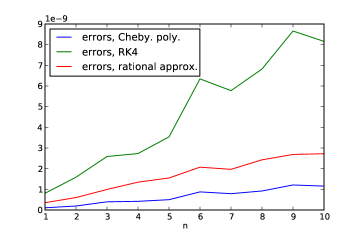
(b)

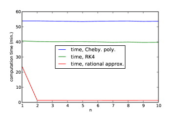
Figure 7. Plot of the $L^{\infty}$ error, $\left\|\mathbf{u}_{n}-e^{n\tau L}\mathbf{u}_{0}\right\|_{\infty}$, versus the big time step $n\tau$, where $\tau=1$ and $1\leq n\leq 300$. Here $\mathbf{u}_{n}$ denotes the numerical approximation to $e^{n\tau L}\mathbf{u}_{0}$, as computed by the rational approximation (5) and the direct solver from Section 2.

Table 2. Comparison of the accuracy and efficiency of applying, $e^{\tau\mathcal{L}}\mathbf{u}_{0}$ and $\tau=1.5$, for system (6) and $\mathbf{u}_{0}$ in (29). The comparison uses RK4, Chebyshev polynomials, and the rational approximation (5); in the spatial discretization of all three comparisons, $12\times 12=144$ elements and $16\times 16=254$ Chebyshev quadrature nodes per element are used.

$e^{\tau\mathcal{L}}$, $\tau=1.5$	$L^{\infty}$ error	time (min.)	pre-comp. (min.)
Rational approx.,	$2.1\times 10^{-10}$	$4.39$	$103.1$
$M=376$ terms
RK4	$7.0\times 10^{-10}$	$131.9$	NA
Cheby. poly.,	$1.1\times 10^{-10}$	$150.5$	NA
degree $12$

We apply the algorithm in the spatial domain $\left[0,1\right]\times\left[0,1\right]$, using periodic boundary conditions and a constant Coriolis force $f=1$ . In this case, an exact solution can be computed analytically since the matrix exponential is diagonalized in the Fourier domain, and can be rapidly applied via the Fast Fourier Transform (FFT). In particular,

$$\mathcal{L}\left(\mathbf{r}_{\mathbf{k}}^{l}e^{i\mathbf{k}\cdot\mathbf{x}}\right)=i\omega_{\mathbf{k}}^{l}\mathbf{r}_{\mathbf{k}}^{l}e^{i\mathbf{k}\cdot\mathbf{x}},$$

where $\mathbf{r}_{\mathbf{k}}^{l}$ are eigenvectors of the matrix

$$\left(\begin{array}[]{ccc}0&-f&igk_{1}\\ -f&0&igk_{2}\\ iHk_{1}&iHk_{2}&0\end{array}\right),$$

and can be found in [16].

We first compare the accuracy and efficiency of applying $e^{n\tau L}\mathbf{u}_{0}$, for $\tau=3$ and $n=1,\ldots,10$, against $4$th order Runge-Kutta (RK4) and against using Chebyshev polynomials. In particular, the Chebyshev method uses the approximation

(28) $$e^{\Delta t\mathcal{L}}\mathbf{u}_{0}\approx J_{0}\left(i\right)\mathbf{u}_{0}+2\sum_{k=0}^{K}\left(i\right)^{k}J_{k}\left(-i\right)T_{k}\left(\Delta t\mathcal{L}\right)\mathbf{u}_{0},$$

coupled with the standard recursion for applying $T_{k}\left(\Delta tL\right)$; we choose a polynomial degree of $12$, which we find experimentally is a good compromise between the time step size $\Delta t$ needed for a given accuracy, and the number of applications of $\mathcal{L}$. In all the time-stepping schemes, we use the same spectral element discretization and parameter values as described above. All the algorithms are implemented in Octave, including the direct solver described in Section 2.

4.1.1. First test case for the shallow water equations

We first consider the initial conditions

$$\eta\left(\mathbf{x}\right) = \sin\left(6\pi x\right)\cos\left(4\pi y\right)-\frac{1}{5}\cos\left(4\pi x\right)\sin\left(2\pi y\right),$$

$$v_{1}\left(\mathbf{x}\right) = \cos\left(6\pi x\right)\cos\left(4\pi y\right)-4\sin\left(6\pi x\right)\sin\left(4\pi y\right),$$

(29) $$v_{2}\left(\mathbf{x}\right) = \cos\left(6\pi x\right)\cos\left(6\pi y\right).$$

For these initial conditions, we use $6\times 6=36$ elements of equal area, and $16\times 16=256$ Chebyshev quadrature nodes for each element. To assess the accuracy of the method, the exponential $e^{n\tau\mathcal{L}}\mathbf{u}_{0}$ is applied in the Fourier domain. When applying the operator exponential using the rational approximation (5), we use $M=376$ inverses and $\tau=3$ ; this results in an $L^{\infty}$ error of $3.4\times 10^{-10}$ for a single (large) time step. For this choice of parameters in the spectral element discretization, the cost of applying the solution operator of (8)—i.e., forming the right hand side of (11), solving (11), and evaluating (10)—is about $4.5$ times more expensive than the cost of applying the forward operator (7) directly.

For the three time-stepping methods, the $L^{\infty}$ errors in the approximation of $e^{n\tau\mathcal{L}}\mathbf{u}_{0}$, $n=1,\ldots,10$, are plotted in Figure 6, (a). Similarly, the total computation times (in minutes) of approximating $e^{n\tau\mathcal{L}}\mathbf{u}_{0}$, $n=1,\ldots,10$, are plotted in Figure 6, (b) (this includes the pre-computation time for representing the inverses). From Figure 6, (a), we see that the $L^{\infty}$ errors from all three methods remain less than $10^{-8}$ for $n=1,\ldots,10$. From Figure 6, (b), we see that the first time step for the rational approximation method is about half the cost of both RK4 and the Chebyshev polynomial method. However, subsequent time steps for the new method is about $40$ times cheaper than both RK4 and the Chebyshev polynomial method (for about the same accuracy).

4.1.2. Second test case: doubling the spatial resolution

Next, we compute $e^{\tau\mathcal{L}}\mathbf{u}_{0}$, $\tau=1.5$, with the initial conditions

$$\eta\left(\mathbf{x}\right) = \sin\left(12\pi x\right)\cos\left(8\pi y\right)-\frac{1}{5}\cos\left(8\pi x\right)\sin\left(4\pi y\right),$$

$$v_{1}\left(\mathbf{x}\right) = \cos\left(12\pi x\right)\cos\left(8\pi y\right)-4\sin\left(12\pi x\right)\sin\left(8\pi y\right),$$

(30) $$v_{2}\left(\mathbf{x}\right) = \cos\left(12\pi x\right)\cos\left(12\pi y\right).$$

In particular, we double the bandlimit in each direction. In each of the time-stepping schemes, we use $12\times 12=144$ elements of equal area, and $16\times 16=256$ Chebyshev quadrature nodes for each element. We again use $M=376$ inverses in (5).

We only examine the error and computation time for one big time step. For the rational approximation method, we present both the pre-computation time for obtaining data-sparse representations of the $376$ inverses in (5), and the computation time for applying the approximation in (5) (once the data-sparse representations are known). The results are summarized in Table 2. Since we only consider a single time step, the pre-computation time and application time are included separately. The main conclusion to draw from these results is that doubling the spatial resolution does not appreciably change the relative efficiency of the three time-stepping methods (once representations for the inverse operators in (5) are pre-computed).

4.1.3. Third test case: applying the operator exponential over a long time interval

Finally, we access the accuracy of the new method when repeatedly applying $e^{\tau\mathcal{L}}$, $\tau=1$, in order to evolve the solution over longer time intervals. In this example, we use the initial conditions

$$\eta\left(\mathbf{x}\right) = \exp\left(-100\left(\left(x-1/2\right)^{2}+\left(y-1/2\right)^{2}\right)\right),$$

$$v_{1}\left(\mathbf{x}\right) = \cos\left(6\pi x\right)\cos\left(4\pi y\right)-4\sin\left(6\pi x\right)\sin\left(4\pi y\right),$$

(31) $$v_{2}\left(\mathbf{x}\right) = \cos\left(6\pi x\right)\cos\left(6\pi y\right).$$

Notice that these initial conditions cannot be expressed as a finite sum of eigenfunctions of $\mathcal{L}$. We use the same spatial discretization parameters as in Section 4.1.2.

In Figure 7, we show the $L^{\infty}$ error of the computed approximation $\mathbf{u}_{n}\left(\mathbf{x}\right)$ to $\mathbf{u}\left(\mathbf{x},n\tau\right)$, $n=1,\ldots,300$. As expected, the error increases linearly in the number of applications of the exponential. Notice that, due to the large step size of $\tau=1$, the error accumulates slowly in time and the solution can be propagated with high accuracy over a large number of characteristic wavelengths.

4.2. Example 2

In our second example, we consider the wave propagation problem

(32) $$u_{tt}=\kappa\Delta u,\,\,\,\,\mathbf{x}\in\left[0,1\right]\times\left[0,1\right],$$

where $\kappa\left(\mathbf{x}\right)>0$ is a smooth function, the initial conditions $u\left(\mathbf{x},0\right)$ and $u_{t}\left(\mathbf{x},0\right)$ are prescribed, and periodic boundary conditions are used.

Table 3. Comparison of the accuracy and efficiency for the operator exponential, $e^{t\mathcal{L}}\mathbf{u}_{0}$ and $t=1.5$, for system (13) and $\mathbf{u}_{0}$ in (33). The comparison uses RK4, Chebyshev polynomials, and the rational approximation (5); in the spatial discretization of all three comparisons, $12\times 12=144$ elements and $16\times 16=254$ Chebyshev quadrature nodes per element are used.

$e^{t\mathcal{L}}$, $t=1.5$	$L^{\infty}$ error	time (min.)	pre-comp. (min.)
Rational approx.,	$1.6\times 10^{-9}$	$3.76$	$113.4$
$M=376$ terms
RK4	$3.5\times 10^{-10}$	$63.9$	NA
Cheby. poly.,	$3.5\times 10^{-8}$	$57.5$	NA
degree $12$

Since the procedure and results are similar to those in Section 4.1, we simply test the efficiency and accuracy of this method over a single time step $\tau=1.5$. In particular, we compare the accuracy and efficiency for one application $e^{\tau\mathcal{L}}\mathbf{u}_{0}$, $\tau=1.5$, against $4$th order Runge-Kutta (RK4) and against using Chebyshev polynomials. In our numerical experiments, we use the initial condition

(33) $$u\left(x,y,0\right)=\sin\left(2\pi x\right)\sin\left(2\pi y\right)+\sin\left(4\pi x\right)\sin\left(4\pi y\right),$$

and $u_{t}\left(x,y,0\right)=0$. We also use

$$\kappa\left(x,y\right)=\left(\frac{3+\sin\left(4\pi x\right)}{4}\right)^{1/2}\left(\frac{3+\sin\left(4\pi y\right)}{4}\right)^{1/2}.$$

Finally, in the spatial discretization, we use $12\times 12=144$ elements with $16\times 16=256$ points per element (for all three time-stepping methods), and $M=376$ poles in (5). For these parameters, the time to apply the inverse of (14)—which involves forming the right hand side in (16), solving for $v$, and computing (15)—is about $5.2$ times more expensive than directly applying the forward operator (13).

Unlike Section 4.1, the operator exponential is not diagonalized in the Fourier domain. To assess the accuracy, we use the Chebyshev polynomial method with a small enough step size to yield an estimated error of less than $10^{-10}$. In particular, we verify that the $L^{\infty}$ residual, $\left\|\mathbf{u}\left(\mathbf{x},t;\Delta t\right)-\mathbf{u}\left(\mathbf{x},t;\Delta t/2\right)\right\|_{\infty}$, using numerical approximations to $\mathbf{u}\left(\mathbf{x},t\right)$ computed with step sizes $\Delta t$ and $\Delta t/2$ and the Chebyshev polynomial method, is less than $10^{-10}$. We then use $\mathbf{u}\left(\mathbf{x},t;\Delta t/2\right)$ as a reference solution.

The results are summarized in Table 3. From this table, we see that the pre-computation time needed to represent the $M=376$ solution operators in (5) is $93$ minutes, and the computation time needed to apply the exponential is $3.7$ minutes; the final accuracy in the $L^{\infty}$ norm is given by $1.6\times 10^{-9}$. For the Chebyshev polynomial method, $575$ time steps of size $\Delta t\approx.0026$ are taken, for an overall time of $57$ minutes; the final accuracy is given by $3.5\times 10^{-8}$. Finally, for RK4, $7,500$ time steps of size $\Delta t=1/5\times 10^{-3}$ are taken, for an overall time of $63.9$ minutes; the final accuracy is $3.5\times 10^{-10}$.

5. Generalizations

The manuscript presents an efficient technique for explicitly computing a highly accurate approximation to the operator $\varphi(\tau\mathcal{L})$ for the case where $\mathcal{L}$ is a skew-Hermitian operator and where $\varphi(t)=e^{t}$, so that $\varphi(\tau\mathcal{L})$ is the time-evolution operator of the hyperbolic PDE $\partial u/\partial t=\mathcal{L}u$. The technique can be extended to more general functions $\varphi$. In particular, in using exponential integrators (cf. [4]), it is desirable to apply functions $\varphi_{j}\left(\tau\mathcal{L}\right)$, where $\varphi_{j}\left(\cdot\right)$ are the so-called phi-functions. In Section 3, we presented (near) optimal rational approximations of the first few phi functions. An important property of these representations is that the same poles can be used to simultaneously apply all the phi-functions, and with a uniformly small error. In particular, linear combinations of the same $2M+1$ solutions $\left(\tau\mathcal{L}-\alpha_{m}\right)^{-1}\mathbf{u}_{0}$, $m=-M,\ldots,M$, can be used to apply $\varphi_{j}\left(\tau\mathcal{L}\right)$ for $j=1,2,\ldots$. In a similar way, linear combinations of the same $2M+1$ solutions can be used to apply $e^{s\mathcal{L}}$ for $0\leq s\leq\tau$.

In addition, where there is a priori knowledge of large spectral gaps—for example, when there is scale separation between fast and slow waves—the techniques in this paper, coupled with those in [12]), can be used to construct efficient rational approximations of $e^{ix}$ which are (approximately) nonzero only where the spectrum of $\mathcal{L}$ is nonzero. Since suitably constructed rational approximations can capture functions with sharp transitions using a small number of poles (see [12]), this approach requires a potentially much smaller number of inverse applications.

Appendix A Error bounds

We now derive the error bound (23). To do so, we use the Poisson summation formula,

$$\sum_{m=-\infty}^{\infty}\Psi_{h}\left(x+mh\right)=\frac{1}{h}\sum_{k=-\infty}^{\infty}e^{2\pi i\left(k/h\right)x}\widehat{\Psi_{h}}\left(\frac{k}{h}\right).$$

Applying this to $\Psi_{h}\left(x\right)=e^{-2\pi ix}\psi_{h}\left(x\right)$, we have that

$$\sum_{m=-\infty}^{\infty}\Psi_{h}\left(x+mh\right) = e^{-2\pi ix}\sum_{m=-\infty}^{\infty}e^{-2\pi imh}\psi_{h}\left(x+mh\right)$$

$$= \frac{1}{h}\sum_{k=-\infty}^{\infty}e^{2\pi i\left(k/h\right)x}\widehat{\Psi_{h}}\left(\frac{k}{h}\right)$$

$$= \frac{1}{h}\sum_{k=-\infty}^{\infty}e^{2\pi i\left(k/h\right)x}\widehat{\psi_{h}}\left(\frac{k}{h}+1\right),$$

where the last inequality uses the fact that

$$\widehat{\Psi_{h}}\left(\frac{k}{h}\right)=\widehat{\psi_{h}}\left(\frac{k}{h}+1\right).$$

Therefore,

$$\left|\sum_{m=-\infty}^{\infty}e^{-2\pi imh}\psi_{h}\left(x+mh\right)-\frac{\widehat{\psi_{h}}\left(1\right)}{h}e^{2\pi ix}\right|\leq\frac{1}{h}\sum_{k\neq 0}\widehat{\psi_{h}}\left(\frac{k}{h}\right).$$

Finally, truncating the sum we obtain the bound (23).

References

- [1] Luca Bergamaschi and Marco Vianello. Efficient computation of the exponential operator for large, sparse, symmetric matrices. Numer. Linear Algebra Appl., 7(1):27–45, 2000.
- [2] G. Beylkin and K. Sandberg. Wave propagation using bases for bandlimited functions. Wave Motion, 41(3):263–291, 2005.
- [3] W. J. Cody, G. Meinardus, and R. S. Varga. Chebyshev rational approximations to in and applications to heat-conduction problems. J. Approximation Theory, 2:50–65, 1969.
- [4] S.M. Cox and P.C. Matthews. Exponential time differencing for stiff systems. Journal of Computational Physics, 176(2):430 – 455, 2002.
- [5] Anil Damle, Gregory Beylkin, Terry Haut, and Lucas Monzon. Near optimal rational approximations of large data sets. Applied and Computational Harmonic Analysis, 35(2):251 – 263, 2013.
- [6] Laurent Demanet and Lexing Ying. Wave atoms and time upscaling of wave equations. Numer. Math., 113(1):1–71, 2009.
- [7] I.S. Duff, A.M. Erisman, and J.K. Reid. Direct Methods for Sparse Matrices. Clarendon Press, Oxford, 1986.
- [8] I. P. Gavrilyuk, W. Hackbusch, and B. N. Khoromskij. Hierarchical tensor-product approximation to the inverse and related operators for high-dimensional elliptic problems. Computing, 74(2):131–157, 2005.
- [9] A. George. Nested dissection of a regular finite element mesh. SIAM J. on Numerical Analysis, 10:345–363, 1973.
- [10] A. Gillman and P.G. Martinsson. A direct solver with complexity for variable coefficient elliptic pdes discretized via a high-order composite spectral collocation method, 2013. arXiv.org report #1307.2665.
- [11] Stefan Guttel. Rational krylov approximation of matrix functions: Numerical methods and optimal pole selection. GAMM-Mitteilungen, 36(1):8–31, 2013.
- [12] T. Haut and G. Beylkin. Fast and accurate con-eigenvalue algorithm for optimal rational approximations. SIAM Journal on Matrix Analysis and Applications, 33(4):1101–1125, 2012.
- [13] T. S. Haut and B. A. Wingate. An asymptotic parallel-in-time method for highly oscillatory PDEs. SIAM J. of Sci. Comput., to appear. See also arXiv:1012.3196 [math.NA], 2013.
- [14] N. Higham. The scaling and squaring method for the matrix exponential revisited. SIAM Journal on Matrix Analysis and Applications, 26(4):1179–1193, 2005.
- [15] M. Hochbruck and C. Lubich. On Krylov subspace approximations to the matrix exponential operator. SIAM J. Numer. Anal., 34(5):1911–1925, 1997.
- [16] Andrew J. Majda. Introduction to PDEs and waves for the atmosphere and ocean. Courant lecture notes in mathematics. Courant Institute of Mathematical Sciences Providence (R.I.), New York, 2003.
- [17] P.G. Martinsson. A direct solver for variable coefficient elliptic {PDEs} discretized via a composite spectral collocation method. Journal of Computational Physics, 242(0):460 – 479, 2013.
- [18] P.G. Martinsson. A direct solver for variable coefficient elliptic pdes discretized via a high-order composite spectral collocation method, a tutorial, 2013. arXiv.org report.
- [19] Vladimir Maz’ya and Gunther Schmidt. On approximate approximations using gaussian kernels. IMA Journal of Numerical Analysis, 16:13–29, 1996.
- [20] Vladimir Maz’ya and Gunther Schmidt. Approximate approximations, volume 141 of Mathematical Surveys and Monographs. American Mathematical Society, Providence, RI, 2007.
- [21] Frank Müller and Werner Varnhorn. Error estimates for approximate approximations with Gaussian kernels on compact intervals. J. Approx. Theory, 145(2):171–181, 2007.
- [22] Nathan Paldor and Andrey Sigalov. An invariant theory of the linearized shallow water equations with rotation and its application to a sphere and a plane. Dynamics of Atmospheres and Oceans, 51(1-2):26 – 44, 2011.
- [23] Thomas Schmelzer and Lloyd N. Trefethen. Evaluating matrix functions for exponential integrators via Carathéodory-Fejér approximation and contour integrals. Electron. Trans. Numer. Anal., 29:1–18, 2007/08.