Department of Physics and Astronomy, Potsdam University, Karl-Liebknecht-Str 24, D-14476, Potsdam, Germany
Laboratoire de Physique Théorique et Modèles Statistiques (CNRS UMR 8626), Université Paris-Sud, Orsay, France
Synchronization; coupled oscillators Phase transitions: general studies Nonequilibrium and irreversible thermodynamics
Synchronization transitions in globally coupled rotors in presence of noise and inertia: Exact results
Abstract
We study a generic model of globally coupled rotors that includes the effects of noise, phase shift in the coupling, and distributions of moments of inertia and natural frequencies of oscillation. As particular cases, the setup includes previously studied Sakaguchi-Kuramoto, Hamiltonian and Brownian mean-field, and Tanaka-Lichtenberg-Oishi and Acebrón-Bonilla-Spigler models. We derive an exact solution of the self-consistent equations for the order parameter in the stationary state, valid for arbitrary parameters in the dynamics, and demonstrate nontrivial phase transitions to synchrony that include reentrant synchronous regimes.
pacs:
05.45.Xtpacs:
05.70.Fhpacs:
05.70.Ln1 Introduction
Synchronization in a large population of coupled oscillators of distributed natural frequencies is a remarkable example of a nonequilibrium phase transition. The paradigmatic minimal model to study synchronization is the one due to Kuramoto, introduced almost 40 years ago [1], based on an earlier work by Winfree [2]. Over the years, many details of the Kuramoto model [3, 4], and applications to various physical [5], chemical [6], biological [7], engineering [8], and even social problems [9] have been addressed in the literature.
The Kuramoto model comprises oscillators that are described by their phases, have natural frequencies given by a common distribution, and are subject to a global mean-field coupling. The phases follow a first-order dynamics in time. In the simplest setup of a purely sinusoidal coupling without a phase shift, and for a unimodal distribution of frequencies, the model exhibits a continuous (second-order) transition from an unsynchronized to a synchronized phase as the coupling constant exceeds a critical threshold. The phase transition appears as a Hopf bifurcation for the complex order parameter.
The dynamics of the Kuramoto model is intrinsically dissipative. When all the oscillators have the same frequency, the analogue of the model in the realm of energy-conserving Hamiltonian dynamics is the so-called Hamiltonian mean-field model (HMF) [10, 11]. In this case, the dynamical equations are the Hamilton equations: the oscillator phases follow a second-order dynamics in time, i.e. the units are in fact not oscillators, but rotors. In order to include the effects of interaction with an external heat bath, it is natural to consider the HMF evolution in presence of a Gaussian thermostat. In the resulting Brownian mean-field (BMF) model, the dynamical equations are damped and noise-driven [12, 13]. Both the HMF and the BMF model have an equilibrium stationary state that exhibits a continuous phase transition between a synchronized phase at low values of energy/temperature and an unsynchronized phase at high values. On considering the BMF model with non-identical oscillator frequencies, the dynamics violates detailed balance leading to a nonequilibrium stationary state (NESS) [14]. In the overdamped limit, the dynamics reduces to that of the noisy Kuramoto model involving Kuramoto dynamics in presence of Gaussian noise, which was introduced to model stochastic fluctuations of the natural frequencies in time [15]. The resulting phase diagram is complex, with both continuous and first-order transitions [14].
In this work, we study a generic model of globally coupled rotors, in which two types of deviations from equilibrium are included: (i) distribution of torques acting on the rotors, similar to the distribution of frequencies in the Kuramoto model, and (ii) a phase shift in the coupling, that makes the latter non-Hamiltonian. We consider the rotors to have quite generally different moments of inertia given by a common distribution [16]. Our setup includes as special cases previously studied Sakaguchi-Kuramoto [17], Hamiltonian and Brownian mean-field, Tanaka-Lichtenberg-Oishi [18], and Acebrón-Bonilla-Spigler [19, 20] models.
The basic roadblock in studying out-of-equilibrium dynamics, in particular, in characterizing the resulting long-time NESSs is the lack of a framework that allows to treat such states on a general footing, akin to the one for equilibrium steady states à la Gibbs-Boltzmann. Even for simple nonequilibrium models, obtaining the steady state distribution has been a tour de force [21], while in many cases, the analytical characterization of the steady state has so far been elusive, thereby requiring one to resort to numerical simulations and approximation methods [22].
In this backdrop, it is remarkable that for our system of study, we are able to characterize exactly the NESS under quite general conditions. In the thermodynamic limit , we study the system by analyzing the Kramers equation for the evolution of the single-rotor phase space distribution. Using the combination of an analytical approach to solve the Kramers equation in the steady state [23] and a novel self-consistency approach [24, 25], we formulate an exact equation for the complex order parameter as a function of the relevant parameters of the system, for arbitrary distributions of torques and moments of inertia. As applications of our approach, we provide for suitable and representative choices of the distribution functions several nontrivial illustrations of transitions to synchrony, including in some cases interesting reentrant synchronous regimes.
2 Basic model
The equations of motion for the -th rotor read
| (1) |
where dots denote differentiation with respect to time . Here, is the angle of the -th rotor with moment of inertia , is the friction constant, is the coupling constant, is the phase shift parameter, is the temperature in units of the Boltzmann constant, while and constitute the complex order parameter of the problem: . Note that is the magnitude while is the phase of the mean field acting on the rotors. In the dynamics (1), the term is the external torque acting on the -th rotor. The parameters of the rotors, namely, their frequencies ’s and the moments ’s, are quenched random variables sampled from a common distribution . The noise is Gaussian, with . To reduce the number of relevant parameters, we introduce dimensionless variables , , , , in terms of which Eq. (1) becomes (with dot now denoting derivative with respect to )
| (2) |
involving two dimensionless parameters and ; here, is a Gaussian white noise with . Additional parameters describe the distribution of dimensionless natural frequencies and moments.
For the dynamics (2), we seek for NESS with non-zero, uniformly-rotating mean field, which generally has a frequency different from the mean frequency of the natural frequencies distribution. Transforming to the reference frame rotating with frequency , as , where is a constant, Eq. (2) reads
| (3) |
with . From now on, we focus on analyzing the dynamics of (3).
At this point, it is instructive to link model (3) to previously studied setups. In the absence of a distribution of frequencies and moments, and for , Eq. (3) describes the BMF model. This model has an equilibrium stationary state in which the system exhibits a continuous phase transition between a synchronized () and an unsynchronized () phase at the critical coupling [12, 13]. Presence of frequencies in the dynamics (3) drives the system to a NESS [14]. For , the dynamics (3) is that of the Sakaguchi-Kuramoto model with the inclusion of noise, which shows a continuous synchronization phase transition across described for in Ref. [15]. In our normalization, the intensity of noise is set to one, thus the noiseless situation corresponds to the limit . For this noiseless dynamics, the case of rotors with the same moments of inertia, and with defines the Tanaka-Lichtenberg-Oishi model [18]. In Ref. [20], for model (2) with and without the distribution of moments (the Acebrón-Bonilla-Spigler model), a linear stability analysis and an approximate treatment of the transition to synchrony have been performed. In both these works, a first-order transition to synchrony was revealed.
3 Thermodynamic limit: The Kramers equation and its self-consistent stationary solution
We now consider the dynamics (3) in the thermodynamic limit . In this limit, the dynamics is characterized by the single-rotor conditional distribution , which gives at time and for the given set of parameters the fraction of rotors with angle and angular velocity . The distribution is -periodic in , and obeys the normalization , while evolving toward a stationary distribution following the Kramers (Fokker-Planck) equation [14]
| (4) |
where we have defined . In the steady state, is time-independent, with
| (5) |
where . The stationary distribution depends on the unknown quantities and , which we from now on consider as given parameters. The representation (5) gives the solution of the problem in a parametric form: the order parameter and the coupling parameters, , are expressed as explicit functions of and , as
| (6) |
By varying and , while keeping the parameters of the distribution fixed, we may find the order parameter as a function of and (cf. [25, 24]).
The stationary solution of the Kramers equation (4) is described in [23]. One looks for a solution in the form of a double expansion in Fourier modes in and Hermite functions in as
| (7) |
where are the Hermite functions: . By inserting expansion (7) into the Kramers equation (4), one obtains a linear system of equations for coefficients which can be solved using matrix continued fraction method [23]. Substituting expansion (7) into Eq. (5), we find that
| (8) |
where denotes complex conjugation. According to the matrix continued fraction method [23], the coefficient can be found from the matrix as
where is given by the following recurrent formula:
| (9) |
with the matrix , while the matrix is
| (10) |
Combining Eqs. (6), (8), (3), (10), one obtains an exact equation for the complex order parameter as a function of the relevant parameters of the system for arbitrary distributions of torques and moments of inertia. In the following sections, we present several applications of our approach to compute the steady state for representative choices of the frequency and moment distribution, and parameters of the dynamics, and highlight possible synchronization transitions.
4 Phase transitions in the case of symmetric coupling function (i.e., )
(a)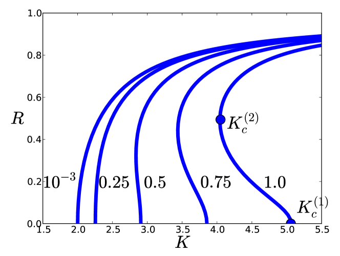
(b)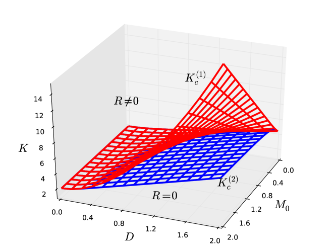
(c)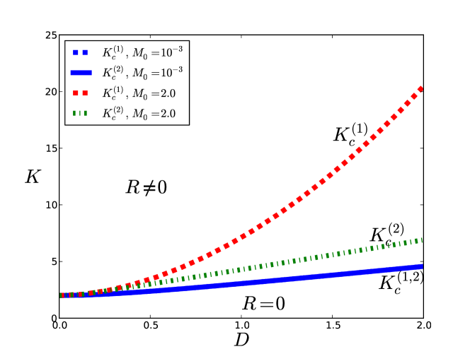
Here, we consider symmetric, Hamiltonian coupling, i.e., with the phase shift . As one can see from (6), the function , given by Eqs. (5) and (8), should be real. Let us choose for each moment the distribution to be symmetric about its mean : . Then, using Eq. (8) and the fact that is real, one arrives at the consistent conclusions that and . (For a general asymmetric distribution, like Eq. (14) below, to be consistent with , one has to vary to find the value at which ). As the simplest example of such a situation, we consider the case of equal moments, and a Gaussian distribution with mean zero and width for the frequencies: , with . In Fig. 1, we report the phase diagram in the three-dimensional space of parameters , stressing on the synchronized and unsynchronized states. The previously known limits are (1) for , when one has the line for continuous transition given by [15], (2) for , when one has the continuous transition point of the BMF model given by , independent of [12, 13]. For , one expects a first-order phase synchronization transition characterized by two thresholds and , where the former is the stability threshold of the unsynchronized phase, while is the point at which two branches of synchronized solutions arise [14]. These observations are borne out by our numerical results depicted in Fig. 1. Panel (a) shows as a function of at a fixed and for different values of : one may observe that at large , the synchronized phase arises as a first-order transition from the unsynchronized phase.
5 Non-universal phase transitions in the case of phase shift in coupling
In this section, we illustrate several examples of non-trivial and non-universal phase transitions to synchrony in the case of nonzero , by choosing , where we choose a nontrivial symmetric that is known to yield a non-universal transition in the Sakaguchi-Kuramoto model [25]:
| (11) |
The results are shown in Fig. 2. Panel (a) shows two examples of a reentrant synchronization transition: with increase of the coupling constant, synchrony first appears but disappears at larger coupling, beyond which there is a second threshold. Fig. 2(b) shows that this behavior depends on the value of in a nontrivial way: while the re-entrance is observed for small and large , it is absent for intermediate values. Finally, in Fig. 2(c) we illustrate how the reentrant behavior depends on noise. As the noise intensity is set to one in our scheme of normalization, we simultaneously varied parameters and according to , , with , . The resulting path in the plane corresponds effectively to variation of the noise intensity, with . One can see that with increase of the noise, the area of nontrivial transitions marked in grey shrinks and disappears. The inset illustrates how the region of the re-entrance is determined from the solution. It shows the values of for vanishing mean field , i.e. at the transition points. At (dashed curve in (c)(inset)), there is a non-monotonic dependence of on . Thus, in the region between the local extrema, there are three values of that give the same value of . These three values correspond to the different branches in each of the plots in Fig. 2(a) at which the value of the order parameter vanishes (i.e. the values of at which synchrony appears, disappears, and appears again). At relatively strong noise (, solid curve in (c)(inset)), there is a monotonic dependence of on , with only one transition to synchrony.
(a)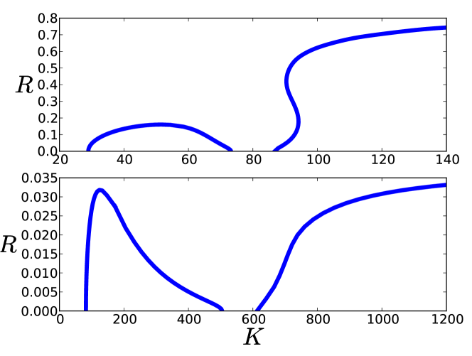
(b)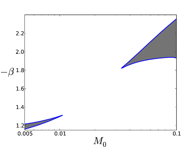
(c)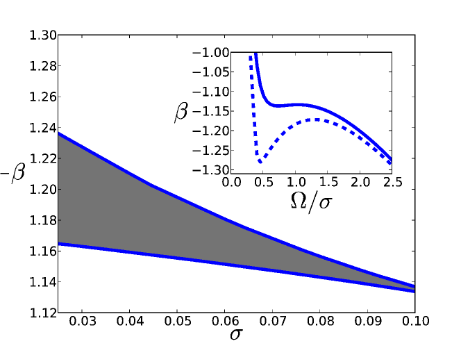
6 Phase transitions in populations with distribution of moments of inertia
(a)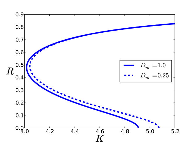
(b)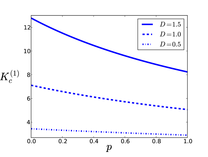
In this section, we present several examples of phase transitions by choosing nontrivial distributions for both moments and frequencies. In the first example, we used independent distributions of moments and frequencies: , with
| (12) |
Thus, the moments are distributed according to a simple parabolic shape with characteristic width ( is the normalization constant), while for frequencies, we use a Gaussian distribution with mean zero and width . In Fig. 3(a), dependencies of the order parameter on the coupling are presented for two distributions for different ’s, but with the same mean moment . One can see that the more diverse is the population, the easier it is to synchronize. To reveal the underlying mechanism, we calculated the synchronization threshold in a more simple setup of rotors having just two different moments, i.e., the distribution is a sum of two delta functions:
| (13) |
where we assume that . By increasing the parameter from 0 to 1, we increase the fraction of light particles in the population. Fig. 3(b) shows that the critical coupling decreases with : One can see that addition of light particles always leads to decreasing of , implying ease of the population to synchronize with more lighter particles; this is consistent with the result in Fig. 3(a).
In the second example we illustrate a situation, where the symmetry of the frequency distribution is broken in a nontrivial way, through a correlation with the moments. We take a distribution
| (14) |
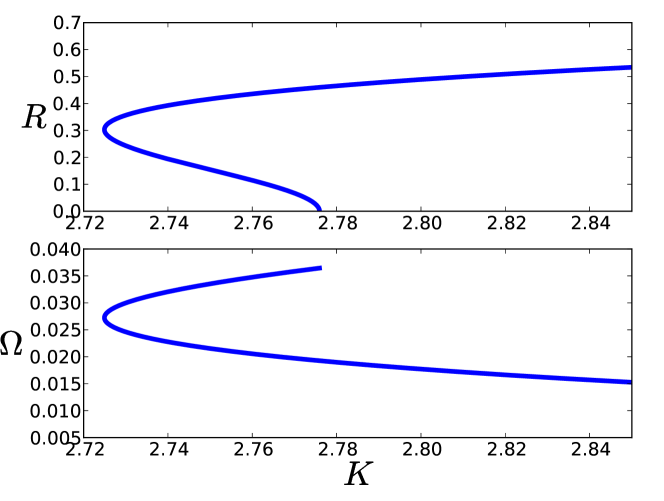
where although the partial distribution of frequencies is symmetric, the overall symmetry of is broken. In this case the frequency of the order parameter will be non-zero even for purely symmetric coupling ; we illustrate this in Fig. 4.
7 Conclusion
In conclusion, we have suggested a unified analytic approach that allows to analyze dynamics of noise-driven populations of globally coupled rotors with a phase shift in the coupling, for arbitrary distribution of their natural frequencies and moments. In addition to well-studied effects of inertia that lead to a first-order transition to synchrony in the absence of a phase shift in coupling, the method allowed us to study more complex regimes. In the limiting case of vanishing inertia and absence of noise, our model reduces to the Sakaguchi-Kuramoto model of coupled phase oscillators. For the latter, reentrant transition to synchrony [25], in which two ranges of coupling exists for observing synchrony, was observed; we demonstrated a similar phenomenon in our model. Furthermore, the general formulation of our model also includes populations with distributions of moments of rotors. A nontrivial effect here is the shift of the frequency of the mean field due to correlations between natural frequencies and the moments.
Acknowledgements.
M. K. thanks the Alexander von Humboldt Foundation for support. S. G. acknowledges the support of the Indo-French Centre for the Promotion of Advanced Research under Project 4604-3, the warm hospitality of the University of Potsdam, and fruitful discussions with A. Campa and S. Ruffo.References
- [1] \NameKuramoto Y. \BookInternational symposium on mathematical problems in theoretical physics (Springer Lecture Notes Phys., New York) 1975.
- [2] \NameWinfree A. T. \REVIEWJ. Theor. Biol.16196715.
- [3] \NameKuramoto Y. \BookChemical Oscillations, Waves and Turbulence (Springer, Berlin) 1984.
- [4] \NameAcebrón J. A., Bonilla L. L., Vicente C. J. P., Ritort F. Spigler R. \REVIEWRev. Mod. Phys.772005137.
- [5] \NameWiesenfeld K., Colet P. Strogatz S. H. \REVIEWPhys. Rev. Lett.761996404.
- [6] \NameAldridge J. Pye E. K. \REVIEWNature2591976670.
- [7] \NameMichaels D. C., Matyas E. P. Jalife J. \REVIEWCirc Res.611987704.
- [8] \NameDörfler F., Chertkov M. Bullo F. \REVIEWPNAS11020132005.
- [9] \NameNéda Z., Nikitin A. Vicsek T. \REVIEWPhysica A3212003238 .
- [10] \NameInagaki S. \REVIEWProg. Theor. Phys.901993577.
- [11] \NameAntoni M. Ruffo S. \REVIEWPhys. Rev. E5219952361.
- [12] \NameChavanis P.-H. \REVIEWPhysica A39020111546 .
- [13] \NameChavanis P. H. \BookThe Brownian mean field model arXiv:1306.1203 (2013).
- [14] \NameGupta S., Campa A. Ruffo S. \REVIEWPhys. Rev. E892014022123.
- [15] \NameSakaguchi H. \REVIEWProg. Theor. Phys.79198839.
- [16] \NameRestrepo J. G. Meiss J. D. \BookOnset of synchronization in the disordered hamiltonian mean field model arXiv:1401.3040 (2014).
- [17] \NameSakaguchi H. Kuramoto Y. \REVIEWProg. Theor. Phys.761986576.
- [18] \NameTanaka H., Lichtenberg A. Oishi S. \REVIEWPhys. Rev. Lett.7819972104.
- [19] \NameAcebrón J. A. Spigler R. \REVIEWPhys. Rev. Lett.8119982229.
- [20] \NameAcebrón J. A., Bonilla L. L. Spigler R. \REVIEWPhys. Rev. E6220003437.
- [21] \NameDerrida B., Evans M. R., Hakim V. Pasquier V. \REVIEWJ. Phys. A: Math. Gen.2619931493.
- [22] \NamePrivman V. \BookNonequilibrium Statistical Mechanics in One Dimension (Cambridge University Press, Cambridge) 2005.
- [23] \NameRisken H. R. \BookThe Fokker–Planck Equation (Springer, Berlin) 1989.
- [24] \NameKomarov M. Pikovsky A. \REVIEWPhys. Rev. Lett.1112013204101.
- [25] \NameOmel’chenko O. E. Wolfrum M. \REVIEWPhys. Rev. Lett.1092012164101.