Coherent excitation of two-state system by a Lorentzian filed

Abstract

This work presents an analytic description of the coherent excitation of a two-state quantum system by an external field with a Lorentzian temporal shape and a constant frequency. An exact analytical solution for the differential equation of the model is derived in terms of Confluent Heun functions. Also a very accurate analytic approximation to the transition probability is derived by using the Dykhne-Davis-Pechukas approach. This approximation provides analytic expressions for the frequency and amplitude of the probability oscillations.

I Introduction

Models involving two-state quantum system has been extensively studied since the early days of quantum mechanics. Nowadays, such models can be found in a variety of problems across quantum physics, ranging from nuclear magnetic resonance, coherent atomic excitation and quantum information to chemical physics, solid-state physics and neutrino oscillations. Moreover, many problems involving multiple states and complicated linkage patterns can very often be understood only by reduction to one or more two-state problems Shore90 . It is known, that the two-state problem with arbitrary time-dependent fields is related to the Riccati equation and hence a general solution cannot be derived.

There are several exactly soluble two-state models, including the Rabi Rabi , Landau-Zener LZ , Rosen-Zener RZ , Allen-Eberly-Hioe AEH , Bambini-Berman BB , Demkov-Kunike DK , Demkov Demkov and Nikitin Nikitin models. Because of the importance of the two-state models, the search for analytical solutions continues Rostovtsev . Due to its complexity most of these models use various special functions to solve the particular two-state problem. If this is not possible, there exist also methods for approximate solutions, such as adiabatic approximations, Magnus approximation, Dykhne-Davis-Pechukas approximation.

In the present work, we derive analytically the transition probability for a two-state system driven by a pulsed external field with Lorentzian temporal envelope and constant carrier frequency. The solution is expressed in terms of confluent Heun functions. This field, for which no exact analytic solution was known yet, is among the most important pulsed fields. Using Delos-Thorson approach presented solution can be extended to solution of class of models Delos-Thorson . Despite the active research the Heun equations and Heun function have not been well studied. Because of this the Lorentzian model will also be investigated with the Dykhne-Davis-Pechukas (DDP) method Dykhne ; Davis76 , which involves integration in the complex time plane, to derive a very accurate approximation to the transition probability and the width of the excitation line profile.

This paper is organized as follows. In Sec. II we provide the basic equations and definitions and define the problem. In Sec. we derive a solution for the differential equation of the model in terms of Confluent Heun functions. In Sec. wederive the transition probability by using the DDP method. We summarize the conclusions in Sec. V.

II Basic equations and definitions

II.1 Definition of the problem

The probability amplitudes in a two-state system $\mathbf{c}(t)=\left[c_{1}(t),c_{2}(t)\right]^{T}$ satisfy the Schrödinger equation,

$$\text{i}\hbar\frac{\text{d}}{\text{d}t}\mathbf{c}(t)=\mathbf{H}(t)\mathbf{c}(t),$$ (1)

where the Hamiltonian in the rotating-wave approximation (RWA) reads B.Shore

$$\mathbf{H}(t)=\tfrac{1}{2}\hbar\left[\begin{array}[]{cc}-\Delta(t)&\Omega(t)\\ \Omega(t)&\Delta(t)\end{array}\right].$$ (2)

The detuning $\Delta$ measures the frequency offset of the field carrier frequency $\omega$ from the Bohr transition frequency $\omega_{0}$, $\Delta=\omega_{0}-\omega$. The Rabi frequency $\Omega(t)$ quantifies the field-induced coupling between the two states. For example, for laser-atom excitation, $\Omega(t)=-\mathbf{d}.\mathbf{E}(t)/\hbar$, where $\mathbf{d}$ is the atomic transition dipole moment and $\mathbf{E}(t)$ is the laser electric field amplitude.

We are interested in the case when the coupling has Lorentzian shape and the detuning is constant,

$$\Omega(t) = \frac{\Omega_{0}}{1+t^{2}/T^{2}},$$ (3a)

$$\Delta(t) = \mathrm{const}.$$ (3b)

Because the transition probability is an even function of $$\Omega_{0} \Delta T$$, and , for simplicity and without loss of generality all these constants will be assumed positive.

If the system is initially in state $|\psi_{1}\rangle$ [$c_{1}(-\infty)=1$, $c_{2}(-\infty)=0$], the transition probability after the interaction is given by $\mathcal{P}=\left|c_{2}(+\infty)\right|^{2}$; its determination is our main concern.

We shall derive below analytic solution for this model al well as several approximations to $\mathcal{P}$ and calculate from them the period and the amplitude of the probability oscillations, the line shape $\mathcal{P}(\Delta)$ and the linewidth $\Delta_{1/2}$.

III Reduction to Heun equation

Heun’s differential equations, which is a second order ODE of Fuchsian type with four regular singular points has received renewed attention, together with its various confluent forms. It turns out the solution of the Lorentzian model is closely related to the confluent Heun equation (CHE). Generally speaking CHE can be obtained from the general Heun equation by coalescing of two of the singular points by redefining certain parameters and taking the appropriate limits. In this way two regular singular points coalesce into one irregular point. For the Lorentzian model this irregular singular point is located at infinity, where the initial conditions are imposed [$c_{1}(-\infty)=1$, $c_{2}(-\infty)=0]$. Although the CHE is relatively well studied [23]-[29], there are essential gaps in the theory and this results to some difficulties when the initial conditions for the Lorentzian model are imposed. In general there are several canonical forms of the CHE. The second order differential equation for the Lorentzian model we intend to solve can be cast to one of the equivalent forms of the CHE-so called generalized spheroidal wave equation (GSWE). Hereafter, we will use the standart form of the GSWE

$$z(z-z_{0})\frac{d^{2}u}{dz^{2}}+\left(B_{1}+B_{2}z\right)\frac{du}{dz}+$$ (4)

$$\left[B_{3}-2\eta\omega(z-z_{0})+\omega^{2}z(z-z_{0})\right]u = 0,$$

where $B_{i\text{ }},\eta$ and $\omega$ are constants with the condition $\omega\neq 0.$ In the GSWE $z=0$ and $z=$ $z_{0}$ are regular singular points with indicial exponents respectively $(0,1+B_{1}/z_{0})$ and $(0,1-B_{2}-B_{1}/z_{0})$. At infinity i.e. $z=\infty$, GSWE has irregular singular point. At this point the behavior of the two independent solutions can be derived from the Thome normal solutions Olver ,Leaver and read

$$\underset{z\rightarrow\infty}{\lim}u(z)\sim e^{\pm i\omega z}z^{\mp i\eta-B_{2}/2}\left(1+O\left(1/z\right)\right)$$ (5)

III.1 Solution in term fo Heun functions

The exact analytical solution for the Lorentzina model can be derived in terms of confluent Heun functions. The differential equation corresponding to Lorentzian model is given by

$$\frac{d^{2}c(t)}{dt^{2}}+\left(\frac{2t}{1+t^{2}}+i\Delta\right)\frac{dc}{dt}+\frac{\Omega_{0}^{2}}{4(1+t^{2})^{2}}c(t)=0.$$ (6)

Using the substitution

$$c(t)=e^{it\Delta}\left(\frac{t+i}{t-i}\right)^{\Omega_{0}/4}u(t)$$

the solution to the Loretnzian differential equation Eq.(6) can be expressed in terms of local confluent Heun functions

$$c(t)=e^{-it\Delta}\left(\frac{t-i}{t+i}\right)^{\Omega_{0}/4}\left[\left(t+i\right)^{\Omega_{0}/2}C_{1}CHl_{1}+C_{2}CHl_{2}\right],$$

where $CHl_{1}$ and $CHl_{2}$ are the local confluent Heun functions as follows

$$CHl_{1} = CHl\left(2\Delta,\frac{\Omega_{0}}{2},\frac{\Omega_{0}}{2},2\Delta,\frac{\Omega_{0}-\Delta}{8};\frac{1-it}{2}\right)$$

$$CHl_{2} = CHl\left(2\Delta,-\frac{\Omega_{0}}{2},\frac{\Omega_{0}}{2},2\Delta,\frac{\Omega_{0}-\Delta}{8};\frac{1-it}{2}\right)$$

IV DDP approach

IV.1 Adiabatic basis

For the derivation of the transition probability we shall need the adiabatic basis, i.e. the basis of the eigenstates of the Hamiltonian (LABEL:Hc). We summarize below the basic definitions and properties of this basis.

In terms of the mixing angle $\vartheta(t)$, defined as

$$\tan 2\vartheta(t)=\frac{\Omega(t)}{\Delta},\qquad(0\leqq\vartheta(t)\leqq\frac{\pi}{4}),$$ (7)

the eigenstates of $\mathsf{H}(t)$ read

$$|\varphi_{-}(t)\rangle = \cos\vartheta(t)|\psi_{1}\rangle-\sin\vartheta(t)|\psi_{2}\rangle,$$ (8a)

$$|\varphi_{+}(t)\rangle = \sin\vartheta(t)|\psi_{1}\rangle+\cos\vartheta(t)|\psi_{2}\rangle.$$ (8b)

The time dependences of the adiabatic states $$|\varphi_{-}(t)\rangle |\varphi_{+}(t)\rangle \vartheta(t) |\psi_{1}\rangle |\psi_{2}\rangle$$ and derive from the mixing angle , whereas the bare (diabatic) states and are stationary.

Because the Rabi frequency $\Omega(t)$ vanishes at large times, and because $\Delta>0$, we have $\vartheta(\pm\infty)=0$; hence

$$|\varphi_{-}(\pm\infty)\rangle = |\psi_{1}\rangle,$$ (9a)

$$|\varphi_{+}(\pm\infty)\rangle = |\psi_{2}\rangle.$$ (9b)

It follows from these relations that a transition between the diabatic states implies a transition between the adiabatic states and vice versa. Hence the transition probability in the adiabatic basis is equal to the transition probability in the diabatic basis.

The energies of the adiabatic states are the eigenvalues of $\mathsf{H}(t)$,

$$\hbar\mathcal{E}_{\pm}(t)=\frac{\hbar}{2}\left[\Delta\pm\sqrt{\Omega^{2}(t)+\Delta^{2}}\right].$$ (10)

The splitting between them is given by

$$\hbar\mathcal{E}(t)=\hbar\mathcal{E}_{+}(t)-\hbar\mathcal{E}_{-}(t)=\hbar\sqrt{\Omega^{2}(t)+\Delta^{2}}.$$ (11)

It tends $\hbar\Delta$ as $t\rightarrow\pm\infty$ and its maximum value $\hbar\sqrt{\Omega_{0}^{2}+\Delta^{2}}$ is reached when $\Omega(t)$ is maximal, at $t=0$.

The probability amplitudes in the diabatic and adiabatic bases are connected via the rotation matrix

$$\mathsf{R}(\vartheta)=\left[\begin{array}[]{cc}\cos\vartheta&\sin\vartheta\\ -\sin\vartheta&\cos\vartheta\end{array}\right],$$ (12)

as

$$\mathbf{c}(t)=\mathsf{R}(\vartheta(t))\mathbf{a}(t),$$ (13)

where the column-vector $\mathbf{a}(t)=[a_{-}(t),a_{+}(t)]^{T}$ comprises the probability amplitudes of the adiabatic states $|\varphi_{-}(t)\rangle$ and $|\varphi_{+}(t)\rangle$. These amplitudes satisfy the transformed Schrödinger equation,

$$i\hbar\frac{d}{dt}\mathbf{a}(t)=\mathsf{H}_{a}(t)\mathbf{a}(t),$$ (14)

where the transformed Hamiltonian is given by

$$\mathsf{H}_{a}(t) = \mathsf{R}^{-1}(\vartheta(t))\mathsf{H}(t)\mathsf{R}(\vartheta(t))-i\hbar\mathsf{R}^{-1}(\vartheta(t))\mathsf{\dot{R}}(\vartheta(t))$$ (17)

$$= \hbar\left[\begin{array}[]{cc}\mathcal{E}_{-}(t)&-i\dot{\vartheta}(t)\\ i\dot{\vartheta}(t)&\mathcal{E}_{+}(t)\end{array}\right],$$

where the overdots denote time derivatives.

IV.2 The Dykhne-Davis-Pechukas approximation

IV.2.1 Single transition point

We shall estimate the transition probability $\mathcal{P}$ for the Gaussian model (3) by using the Dykhne-Davis-Pechukas (DDP) approximation. The DDP formula Dykhne ; Davis76 provides the asymptotically exact transition probability between the adiabatic states in the adiabatic limit. We shall use this formula to calculate the transition probability $\mathcal{P}$ in the original, diabatic basis because, as we discussed above, the transition probabilities in the adiabatic and diabatic bases are equal. The DDP formula reads

$$\mathcal{P}\sim e^{-2\mathrm{Im}\mathcal{D}(t_{0})},$$ (18)

where

$$\mathcal{D}(t_{0})=\int_{0}^{t_{0}}\mathcal{E}(t)dt.$$ (19)

The point $t_{0}$ is called the transition point and it is defined as the (complex) zero of the quasienergy splitting,

$$\mathcal{E}(t_{0})=0,$$ (20)

which lies in the upper half of the complex $t$-plane (i.e., with $\mathrm{Im\,}t_{0}>0$). Equation (18) gives the correct asymptotic probability for nonadiabatic transitions provided: (i) the quasienergy splitting $\mathcal{E}(t)$ does not vanish for real $t$, including at $\pm\infty$; (ii) $\mathcal{E}(t)$ is analytic and single-valued at least throughout a region of the complex $t$-plane that includes the region from the real axis to the transition point $t_{0}$; (iii) the transition point $t_{0}$ is well separated from the other quasienergy zero points (if any) and from possible singularities; (iv) there exists a level (or Stokes) line defined by

$${\text{Im}}\mathcal{D}(t)={\text{Im}}\mathcal{D}(t_{0}),$$ (21)

which goes from $-\infty$ to $+\infty$ and passes through $t_{0}$.

As has been pointed out already by Davis and Pechukas Davis76 , for the Landau-Zener model LZ , which possesses a single transition point, the DDP formula (18) gives the exact transition probability, not only in the adiabatic limit but also in the general case. This amazing feature indicates not only the relevance of the DDP approximation, but raises an intriguing, yet unanswered question: how can a (first-order) approximate method provide the exact solution?

IV.2.2 Multiple transition points

In the case of more than one zero points in the upper $t$-plane, Davis and Pechukas Davis76 have suggested, following George and Lin George74 , that Eq. (18) can be generalized to include the contributions from all these $N$ zero points $t_{k}$ in a coherent sum. This suggestion has been later verified by Joye et al. Joye91 and Suominen et al. Suominen91 ; Suominen92pra ; Suominen92oc ; SuominenThesis . The generalized DDP formula has the form

$$\mathcal{P}\sim\left|\sum_{k=1}^{N}\Gamma(t_{k})e^{i\mathcal{D}(t_{k})}\right|^{2},$$ (22)

where $\Gamma(t_{k})$ are phase factors defined by

$$\Gamma(t_{k})=4i\lim\limits_{t\rightarrow t_{k}}(t-t_{k})\dot{\vartheta}(t).$$ (23)

In principle, Eq. (22) should be used when there are more than one transition points lying on the lowest Stokes line (the closest one to the real axis) and should include in principle only the contributions from these points; moreover, Eq. (22) has been rigorously proved only for these transition points Joye91 .

Another open question for the DDP method is the parameter range where it applies. Strictly, the DDP approximation, being a perturbative result in the adiabatic basis, should be valid only near the adiabatic limit. For a Gaussian field this implies the range defined by the adiabatic condition (LABEL:adiabatic_condition_Gaussian). However, we shall see that the DDP approximation describes very accurately the transition probability well outside this range, virtually for any parameter values, which follows similar earlier successes of this approximation for other models (for some of which, as we discussed, it provides even the exact result). This accuracy of the DDP approximation well beyond the adiabatic regime, essentially in the entire parameter plane, is another open question.

IV.3 Transition points

For the Lorentzian model (3), the transition points in the upper half-plane in terms of the dimensionless time $\tau=t/T$ are given by

$$\tau^{\pm}=\pm\sqrt{\frac{-1+\sqrt{1+\alpha^{2}}}{2}}+i\sqrt{\frac{1+\sqrt{1+\alpha^{2}}}{2}},$$ (24)

where

$$\alpha=\frac{\Omega_{0}}{\Delta}.$$ (25)

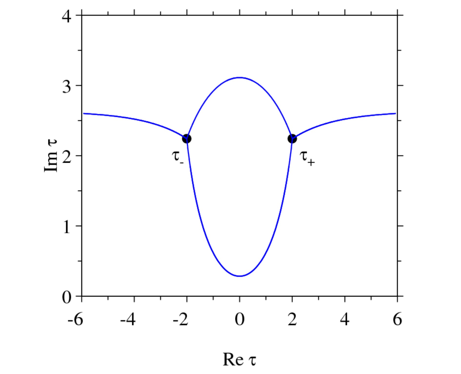
Figure 1: Stokes lines for the Lorentzian model

Figure 1 displays the Stokes lines, defined by Eq. (21). For the Lorentzian model the zeroes of the eigenenergy splitting $\mathcal{E}(t)$ are simple, and because of the presence of the square root in $\mathcal{E}(t)$, there are three Stokes lines emerging from each transition point Davis76 . The lowest Stokes line, which connects $\tau^{-}$ and $\tau^{+}$ and extends from $-\infty$ to $+\infty$, is the most significant one because it is used in the derivation of the DDP approximation Davis76 and its existence validates the approximation Joye91 .

IV.4 DDP integrals

For the Lorentzian model we have $\left(\tau^{-}\right)^{\ast}=-\tau^{+}$ and because $\mathcal{E}(\tau)$ is an even function of time, it is easy to show that

$$\mathcal{D}(\tau^{-})=-\mathcal{D}^{\ast}(\tau^{+}),$$ (26)

that is ${\text{Re}}\mathcal{D}(\tau^{-})=-{\text{Re}}\mathcal{D}(\tau^{+})$ and ${\text{Im}}\mathcal{D}(\tau^{-})={\text{Im}}\mathcal{D}(\tau^{+})$. Hence it is sufficient to calculate only one of these integrals and we choose $\mathcal{D}(\tau^{+})$ for this purpose.

Because the imaginary part of the DDP integral $\mathcal{D}(\tau)$ is the same for the two transition points $\tau^{+}$ and $\tau^{-}$ [cf. Eq. (26)], these points lie on the same Stokes line, defined by Eq. (21). This Stokes line extends from $-\infty$ to $+\infty$, which is a necessary condition for the validity of the DDP approximation Davis76 ; Joye91 .

With the arguments presented above, the problem is reduced to the calculation of the DDP integral

$$\mathcal{D}(\tau^{+})=\Delta T\int_{0}^{\tau^{+}}\frac{\sqrt{\alpha^{2}+\left(1+\tau^{2}\right)^{2}}}{1+\tau^{2}}\,d\tau.$$ (27)

It is well known that integrals of the form $\int R[t,\sqrt{P(t)}]dt,$ where $P(t)$ is a polynomial of third or fourth degree and $\ R$ is a rational function can be solved in terms of three Legendre’s canonical elliptic integrals. These fundamental integrals are denoted as $E(\varphi,k),$ $F(\varphi,k)$ and $\Pi(n;\varphi,k)$

$$E(\varphi,k) = \int_{0}^{\varphi}\sqrt{1-k\sin^{2}t}dt$$ (28a)

$$F(\varphi,k) = \int_{0}^{\varphi}1/\sqrt{1-k\sin^{2}t}dt$$ (28b)

$$\Pi(n;\varphi,k) = \int_{0}^{\varphi}1/\sqrt{(1-n\sin^{2}t)(1-k\sin^{2}t)}dt$$ (28c)

Elliptic integrals . It is straightforward calculation to obtain the following expression for the integral given by (27)

$$\mathcal{D}(\tau^{+})=\frac{\Delta T}{\sqrt{1-i\alpha}}\left[\left(-i-\alpha\right)E(\varphi,k)+\alpha F(\varphi,k)-i\alpha^{2}\Pi(n;\varphi,k)\right],$$ (29)

where $n,\varphi$ and $k$ are given by

$$\varphi=i\arcsin\text{h}\left(\frac{\tau^{+}}{\sqrt{2+2i\alpha}}\right);\ k=\frac{1+i\alpha}{1-i\alpha};\;n=1+i\alpha.$$ (30)

IV.5 Transition probability

In order to sum the contributions from the two DDP integrals we need the factors $\Gamma_{k}$, Eq. (23). One finds after simple algebra that

$$\Gamma(\tau^{\pm})=\pm 1.$$ (31)

Now we have all the ingredients to calculate the transition probability $\mathcal{P}$. Collecting the results from Eqs. (29) and (31) we find

$$\mathcal{P}\sim 4\exp\left[-2{\text{Im}}\mathcal{D}(\tau^{+})\right]\sin^{2}\left[{\text{Re}}\mathcal{D}(\tau^{+})\right].$$ (32)

We replace this expression by

$$\mathcal{P}\sim\frac{\sin^{2}\left[{\text{Re}}\mathcal{D}(\tau^{+})\right]}{\cosh^{2}\left[{\text{Im}}\mathcal{D}(\tau^{+})\right]}.$$ (33)

There are several arguments in favour of this replacement. First of all, the error we make when replacing Eq. (32) with (33) is comparable or smaller, and therefore negligible within the adiabatic limit, where the DDP approximation itself is rigorously proved. Second, Eq. (33) is superior to Eq. (32) because it does not violate unitarity ($\mathcal{P}\leqq 1$), whereas Eq. (32) does (albeit only outside its range of validity). Lastly, such a replacement has already been used Crothers and shown to improve the accuracy.

V Conclusions

We have examined the coherent excitation of two-state quantum system by external pulsed field with Lorentzian temporal shape. The solution of the problem can be expressed in terms of confluent Heun functions (CHF), but due to some limitation of the analytical results for the CHF, analytical approximation for the model is derived using DDP method.

- (1) B. W. Shore, The Theory of Coherent Atomic Excitation (Wiley, New York, 1990).
- (2) I. I. Rabi, Phys. Rev. 51, 652 (1937).
- (3) L. D. Landau, Physik Z. Sowjetunion 2, 46 (1932); C. Zener, Proc. R. Soc. Lond. Ser. A 137, 696 (1932).
- (4) N. Rosen and C. Zener, Phys. Rev. 40, 502 (1932).
- (5) L. Allen and J. H. Eberly, Optical Resonance and Two-Level Atoms (Dover, New York, 1987); F. T. Hioe, Phys. Rev. A 30, 2100 (1984).
- (6) A. Bambini and P. R. Berman, Phys. Rev. A 23, 2496 (1981).
- (7) Yu. N. Demkov and M. Kunike, Vestn. Leningr. Univ. Fiz. Khim. 16, 39 (1969); see also F. T. Hioe and C. E. Carroll, Phys. Rev. A 32, 1541 (1985); J. Zakrzewski, Phys. Rev. A 32, 3748 (1985); K.-A. Suominen and B. M. Garraway, Phys. Rev. A 45, 374 (1992).
- (8) Yu. N. Demkov, Sov. Phys.-JETP 18, 138 (1964).
- (9) E. E. Nikitin, Opt. Spectrosc. 13, 431 (1962); E. E. Nikitin, Discuss. Faraday Soc. 33, 14 (1962); E. E. Nikitin, Adv. Quantum Chem. 5, 135 (1970).
- (10) P. K. Jha1 and Y. V. Rostovtsev, Phys. Rev. A 82, 015801 (2010).
- (11) J. B. Delos and W. R. Thorson, Phys. Rev. A 6, 728 (1972).
- (12) A. M. Dykhne, Sov. Phys. JETP 11, 411 (1960); Sov. Phys. JETP 14, 941 (1962).
- (13) J. P. Davis and P. Pechukas, J. Chem. Phys. 64, 3129 (1976).
- (14) F. M. J. Olver, Asymptotics and Special Functions (Academic Press, New York, 1974).
- (15) E. W. Leaver, J. Math. Phys. 27 (1986) 1238-1265.
- (16) J. V. Armitage, W. F. Eberlein, Elliptic functions (CUP, 2006); M. Abramowitz , I. A. Stegun (eds.), Handbook of mathematical functions (10ed., NBS, 1972).
- (17) G. F. Thomas, Phys. Rev. A 27, 2744 (1983).
- (18) E. Bava, A. Godone, C. Novero, H. O. Di Rocco, Phys. Rev. A 45, 1967 (1992).
- (19) P. R. Berman, L. Yan, K.-H. Chiam, R. Sung, Phys. Rev. A 57, 79 (1998).
- (20) T. F. George and Y.-W. Lin, J. Chem. Phys. 60, 2340 (1974).
- (21) A. Joye, G. Mileti, C.-E. Pfister, Phys. Rev. A 44, 4280 (1991).
- (22) K.-A. Suominen, B. M. Garraway, and S. Stenholm, Opt. Commun. 82, 260 (1991).
- (23) K.-A. Suominen and B. M. Garraway, Phys. Rev. A 45, 374 (1992).
- (24) K.-A. Suominen, Opt. Commun. 93, 126 (1992).
- (25) K.-A. Suominen, Ph.D. thesis (University of Helsinki, Finland, 1992).
- (26) N. V. Vitanov and K.-A. Suominen, Phys. Rev. A 59, 4580 (1999).
- (27) M. Abramowitz and I. A. Stegun, Handbook of Mathematical Functions (Dover, New York, 1964).
- (28) R. B. Dingle, Asymptotic Expansions: Their Derivation and Interpretation (Academic, London, 1973).
- (29) D. S. F. Crothers, J. Phys. A 5, 1680 (1972); J. Phys. B 6, 1418 (1973).
- (30) U. Gaubatz, P. Rudecki, S. Schiemann, K. Bergmann, J. Chem. Phys. 92, 5363 (1990); S. Schiemann, A. Kuhn, S. Steuerwald, K. Bergmann, Phys. Rev. Lett. 71, 3637 (1993).
- (31) N. V. Vitanov, M. Fleischhauer, B. W. Shore and K. Bergmann, Adv. At. Mol. Opt. Phys. 46, 55 (2001); N. V. Vitanov, T. Halfmann, B. W. Shore and K. Bergmann, Ann. Rev. Phys. Chem. 52, 763 (2001).
- (32) M. Hennrich, T. Legero, A. Kuhn and G. Rempe, Phys. Rev. Lett. 85, 4872 (2000); A. Kuhn, M. Hennrich, and G. Rempe, Phys. Rev. Lett. 89, 067901 (2002).
- (33) Z. Kis and F. Renzoni, Phys. Rev. A 65, 032318 (2002); X. Lacour, S. Guérin, N. V. Vitanov, L. P. Yatsenko and H. R. Jauslin, Opt. Commun. 264, 362 (2006); C. Wunderlich, T. Hannemann, T. Körber, H. Häffner, C. Roos, W. Hänsel, R. Blatt and F. Schmidt- Kaler, J. Mod. Opt. 54, 1541 (2007).
- (34) M. A. Nielsen and I. L. Chuang, Quantum Computation and Quantum Information (Cambridge University Press, 1990).
- (35) P. W. Shor, 37th Symposium on Foundations of Computing 56–65 (IEEE Computer Society Press, Washington DC, 1996); A. Steane, Rep. Prog. Phys. 61, 117 (1998); E. Knill, Nature 434, 39 (2005); J. Benhelm, G. Kirchmair, C. F. Roos and R. Blatt, Nature Phys. 4, 463 (2008).
- (36) S. Guérin, S. Thomas, and H. R. Jauslin, Phys. Rev. A 65, 023409 (2002); X. Lacour, S. Guérin and H. R. Jauslin, Phys. Rev. A 78, 033417 (2008).
- (37) J. P. Davis and P. Pechukas, J. Chem. Phys. 64, 3129 (1976); A. M. Dykhne, Sov. Phys. JETP 11, 411 (1960).
- (38) B. W. Shore, The Theory of Coherent Atomic Excitation (Wiley, New York, 1990).
- (39) T. A. Laine and S. Stenholm, Phys. Rev. A 53, 2501 (1996).
- (40) N. V. Vitanov and S. Stenholm, Opt. Commun. 127, 215 (1996).
- (41) K. Drese and M. Holthaus, Eur. Phys. J. D , 73 (1998).
- (42) P. Marte, P. Zoller and J. L. Hall, Phys. Rev. A 44, R4118 (1991).
- (43) N. V. Vitanov, K.-A. Suominen and B. W. Shore, J. Phys. B: At. Mol. Opt. Phys. 32, 4535 (1999).
- (44) T. Wilk, S. C. Webster, H. P. Specht, G. Rempe, and A. Kuhn, Phys. Rev. Lett. 98, 063601 (2007); A. Kuhn, M. Hennrich, and G. Rempe, Phys. Rev. Lett. 89, 067901, (2002).