Non-Local Priors for High-Dimensional Estimation
Abstract
Simultaneously achieving parsimony and good predictive power in high dimensions is a main challenge in statistics. Non-local priors (NLPs) possess appealing properties for high-dimensional model choice, but their use for estimation has not been studied in detail. We show that, for regular models, Bayesian model averaging (BMA) estimates based on NLPs shrink spurious parameters either at fast polynomial or quasi-exponential rates as the sample size increases (depending on the chosen prior density). Non-spurious parameter estimates only differ from the oracle MLE by a factor of . We extend some results to linear models with dimension growing with . Coupled with our theoretical investigations, we outline the constructive representation of NLPs as mixtures of truncated distributions. From a practitioners’ perspective, our work enables simple posterior sampling and extending NLPs beyond previous proposals. Our results show notable high-dimensional estimation for linear models with at reduced computational cost. NLPs provided lower estimation error than benchmark and hyper-g priors, SCAD and LASSO in simulations, and in gene expression data achieved higher cross-validated with an order of magnitude less predictors. Remarkably, these results were obtained without the need to pre-screen predictors. Our findings contribute to the debate of whether different priors should be used for estimation and model selection, showing that selection priors may actually be desirable for high-dimensional estimation.
Keywords: Model Selection, MCMC, Non Local Priors, Bayesian Model Averaging, Shrinkage
1 Introduction
Developing high-dimensional methods that balance parsimony and good predictive power is a main challenge in statistics. Non-local prior (NLP) distributions have appealing properties for Bayesian model selection. Relative to local priors (LPs), NLPs discard spurious covariates faster as the sample size grows, while preserving exponential learning rates to detect non-zero coefficients (?). As shown below, when combined with Bayesian model averaging (BMA), this extra shrinkage has important consequences for parameter estimation. Denote the observations by , where is the sample space. We entertain a collection of models for with Radon-Nikodym densities , where are parameters of interest and is a fixed-dimension nuisance parameter. We assume that models are nested in (), has 0 Lebesgue measure for , denote and . A prior density for under is a NLP if it converges to 0 as approaches any value consistent with a sub-model .
Definition 1.
Let , an absolutely continuous is a non-local prior if for any , .
For preciseness, we assume that any for some . To fix ideas, we consider variable selection where for a given function and predictors and by setting elements in to 0. We entertain the following NLP densities
| (1) | |||
| (2) | |||
| (3) |
where are the non-zero coefficients, is the univariate Normal density with mean and variance and , and are called the product MOM, iMOM and eMOM priors (pMOM, piMOM and peMOM, respectively). Consider the usual BMA estimate
| (4) |
where and is the integrated likelihood under . BMA shrinks estimates by assigning small to unnecessarily complex models. Let be the smallest model such that minimizes Kullback-Leibler (KL) divergence to the data-generating density for some . Under regular models with fixed and , if is a LP and then and if then (?). Models containing spurious parameters are hence regularized at a slow polynomial rate, which implies that if truly then (Section 2), where depends on ratios of model prior probabilities. We shall show that any LP can be transformed into a NLP to achieve either (pMOM) or (peMOM, piMOM). A complementary strategy is to penalize complex models via . For instance, ? and ? consider multiple Normal means and linear regression in a fully Bayesian framework where variable inclusion probabilities decrease with , and show that certain induce shrinkage at optimal asymptotic minimax rates, in particular finding that light-tailed priors (e.g. Normal) are sub-optimal. ? propose a related empirical Bayes strategy. Yet another option is to consider the single model and specify absolutely continuous shrinkage priors, which can also achieve good posterior concentration (?). For a related review on penalized-likelihood strategies see ?.
In contrast, our strategy is based upon faster rates and (optionally) sparsity-inducing . To illustrate the key role of NLPs, in Normal regression models with , and bounded then when using NLPs and to 0 when using LPs (?). We note that when sparse are used consistency may still be achieved with LPs, e.g. ? or ? prove consistency in linear regression with prior inclusion probabilities for . While both and induce sparsity, we note that the latter is guided by strong a priori assumptions.
The main contribution of this manuscript is two-fold. First, we characterize complexity penalties and implied asymptotic rates for BMA estimates induced by NLPs (Section 2). Second, we provide a one-to-one representation of NLPs as mixtures of truncated distributions (Section 3) that addresses important practical issues. It provides an intuitive justification for NLPs, adds flexibility in prior choice and facilitates posterior sampling under strong multi-modalities (Section 4). Finally, we study finite-sample performance in simulations and gene expression data (Section 5).
2 Non local priors for estimation
 |
 |
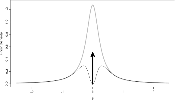 |
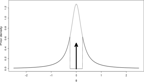
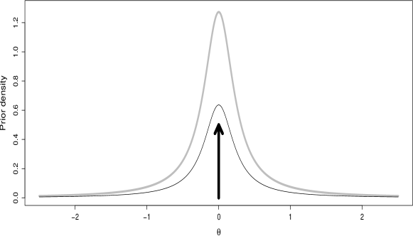
We provide intuition with a simple example. Suppose we wish to both estimate and test vs. , and that we are comfortable with a (possibly vague) prior for the estimation problem. Figure 1 (grey line) shows a prior expressing confidence that is close to 0, e.g. . A testing prior assigns positive , but to be consistent we aim to preserve the estimation prior as much as possible. We set a practical significance threshold and combine a point mass at 0 with a truncated to exclude , with (Figure 1(top), black line). This assigns the same as before for and concentrates all probability in at . Truncated priors have been discussed before (?; ?; ?). They encourage coherence between estimation and testing, but they cannot detect small but non-zero coefficients. Instead, most Bayesian tests use non-truncated priors (?; ?; ?; ?; ?; ?; ?; ?). Figure 1 (middle) combines a with a point mass at 0. It is much more concentrated around 0, e.g. decreased from 0.5 to 0.25. We view this discrepancy between estimation and testing priors as troublesome, as their underlying beliefs cannot be easily reconciled. Suppose that we go back to the truncated Cauchy and set () to express our uncertainty about . Figure 1 (bottom) shows the marginal prior on after integrating out . It is a smooth version of the truncated Cauchy that goes to 0 as , showing an example where a NLP arises as a mixture of truncated distributions (see Section 3). Relative to the estimation prior, most of the probability assigned to is absorbed by the point mass, and is roughly preserved for . An advantage is that testing and estimation are conducted under the same framework. Also, as we now show induces strong shrinkage.
We note that any NLP can be written as , where as for any and is a LP. To ensure that is proper we assume . NLPs are often expressed in this form ((1) or (3)), but the representation is always possible since . Throughout we assume that is bounded for all . The following result guarantees that under NLPs induce an additional penalization for overly complex models. All proofs are provided in the Appendix.
Proposition 1.
Let be the integrated likelihoods for a NLP and the corresponding LP under model for , as above. For ,
-
(i)
Let be the mean of under the LP posterior. Then .
-
(ii)
Consider the peMOM or piMOM priors under with fixed . Let be such that for any minimizes KL divergence to the data-generating density , and assume that for any as
If is a singleton (identifiable models) then . For any , if for some then when , and when either or . The results also hold if is the pMOM prior and as , where is the integrated likelihood under a Normal prior with dispersion and .
That is, NLPs add a term that converges to 0 for unnecessarily complex models and to a finite constant otherwise. The conditions in (ii) essentially require MLE consistency (see ? for general conditions that include non-identifiable models). The pMOM condition on is equivalent to the ratio of posterior densities under and at an arbitrary converging to a constant (see proof). This typically holds, e.g. under the conditions in ? for asymptotic posterior normality or the linear models in Proposition 2, where we allow the number of variables to grow arbitrarily fast with , but only models with variables are considered, (). Specifically, let with under and . Let , and be the least squares estimate.
Proposition 2.
Let be a NLP where either or with for all and some constant . Assume that there exist fixed such that for all , where denote the smallest and largest eigenvalues of . Let minimize KL divergence to the data-generating density with . Further, assume that is continuous, bounded and . Then
Further, if the true density for some then with when and when .
We note that the eigenvalue conditions are strongly related to MLE consistency (?). So far we saw that NLPs improve model selection via an extra complexity penalty. We now turn attention to parameter estimates conditional on a given .
Proposition 3.
Let with fixed satisfy the conditions in ?. Let be an MLE and minimize KL divergence to data-generating density .
-
(i)
Let be the posterior mode such that for all under either a pMOM, peMOM or piMOM prior. If , then for some for the pMOM, peMOM and piMOM priors. If then for pMOM and for peMOM and piMOM and (distinct) . Further, if the MLE is unique then any other posterior mode is (pMOM) or (peMOM, piMOM).
-
(ii)
The posterior mean under a pMOM and under a peMOM or piMOM prior.
-
(iii)
Let satisfy the conditions in Proposition 2 with , and diagonal . Then the rates in (i)-(ii) remain valid.
Conditional on spurious parameter estimates under NLPs converge to 0 at either the same (pMOM) or slightly slower rate (peMOM,piMOM) than the MLE. As shown in the next proposition, BMA combines these estimates with weights to achieve fast polynomial (pMOM) or quasi-exponential shrinkage rates (peMOM,piMOM).
Proposition 4.
Let be the BMA posterior mean in (4), the Bayes factor between and and the MLE of under .
-
(i)
Assume that all satisfy Walker’s conditions and is fixed. Denote by the data-generating model and assume that for any such that . If then under a pMOM, peMOM or piMOM prior. If then under a pMOM prior and under either a peMOM or piMOM prior.
-
(ii)
Assume the conditions in (i) and that . Let where , . If then under pMOM, peMOM or piMOM priors. If then under pMOM priors
and under peMOM or piMOM priors
-
(iii)
Consider linear models as in Proposition 3(iii) and known residual variance . Let for and assume that the prior is exchangeable. If then for pMOM, peMOM and piMOM. If then for pMOM and for peMOM and piMOM.
When setting in the pMOM prior the for spurious coefficients becomes , and should be compared to an shrinkage obtained with LPs. Interestingly, this term only affects spurious coefficients (asymptotically). The result also clarifies the role of sparse in inducing even stronger shrinkage.
3 Non-local priors as truncation mixtures
We establish a correspondence between NLPs and truncation mixtures. Our discussion is conditional on , hence for simplicity we omit and denote , . All proofs are in the Appendix.
3.1 Equivalence between NLPs and truncation mixtures
We show that truncation mixtures define valid NLPs, and subsequently that any NLP may be represented in this manner. Given that the representation is not unique, we give two constructions and discuss their merits. Let be a LP on and a latent truncation point.
Proposition 5.
Define , where for any , and is bounded in a neighborhood of . Let be a marginal prior for placing no probability mass at . Then defines a NLP.
Corollary 1.
Assume that . Let where have an absolutely continuous prior . Then is a NLP.
This alternative representation can be convenient for sampling (as illustrated later on) or to avoid the marginal dependency between elements in induced by a common truncation.
Example 1.
Consider , where , is known and is the identity matrix. We define a NLP for with a single truncation point with and some , e.g. Gamma or Inverse Gamma. Obviously, the choice of affects (Section 3.2). An alternative prior is , giving marginal independence when has independent components.
We address the reverse question: given any NLP, a truncation representation is always possible.
Proposition 6.
Let be an arbitrary NLP and denote , where is the probability under . Then is the marginal prior associated to and where is the expectation with respect to .
Corollary 2.
Let be a NLP, and assume that . Then is the marginal prior associated to and .
The advantage of Corollary 2 is that, in spite of introducing additional latent variables, it greatly facilitates sampling. The condition that is guaranteed when has independent components (apply Proposition 6 to each univariate marginal).
Example 2.
The pMOM prior with , can be represented as and
where is the survival function for a product of independent chi-square random variables with 1 degree of freedom (?). Prior draws are obtained by
-
1.
Draw . Set , where is the cdf associated to .
-
2.
Draw .
As drawbacks, requires Meijer G-functions and is cumbersome to evaluate for large and sampling from a multivariate Normal with truncation region is non-trivial.
 |
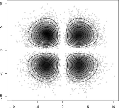 |
Corollary 2 gives an alternative. Let be the cdf associated to where is the survival of a distribution. For , draw , set and draw . The function can be tabulated and quickly evaluated, rendering efficient computations. Figure 2 shows 100,000 draws from univariate (left) and bivariate (right) pMOM priors with .
3.2 Deriving NLP properties for a given mixture
We establish how two important characteristics of a NLP functional form, the penalty and its tail behavior, depend on a given truncation scheme. It is necessary to distinguish whether a single or multiple truncation variables are used.
Proposition 7.
Let be the marginal NLP for , where , is absolutely continuous and . Denote .
-
(i)
Consider any sequence such that . Then
for some . If then .
-
(ii)
Let be any sequence such that . Then where is either a positive constant or . In particular, if then .
Property (i) is important as asymptotic Bayes factor rates depend on the form of the penalty, given by and hence only depending on the smallest . Property (ii) shows that inherits its tail behavior from . Corollary 3 is an extension to multiple truncations.
Corollary 3.
Let be the marginal NLP for , where under and is absolutely continuous.
-
(i)
Let such that for . Then for some , .
-
(ii)
Let such that for . Then where is either a positive constant or . In particular, if under the prior on , then .
That is, multiple independent truncation variables give a multiplicative penalty and tails are at least as thick as those of . Once a functional form for is chosen, we need to set its parameters. Although the asymptotic rates (Section 2) hold for any fixed parameters, their value can be relevant in finite samples. Given that posterior inference depends solely on the marginal prior , whenever possible we recommend eliciting directly. For instance, ? defined practical significance in linear regression as signal-to-noise ratios , and gave default assigning . ? found analogous for probit regression, and also considered learning either via a hyper-prior or minimizing posterior predictive loss (?). ? devised objective Bayes strategies. Yet another possibility is to match the unit information prior e.g. setting , which can be regarded as minimally informative (in fact for the MOM default ). When is not in closed-form prior elicitation depends both on and , but prior draws can be used to estimate for some or . An analytical alternative is to set so that when , i.e. matches a practical relevance threshold. For instance, for and under the MOM prior we would set , and under the eMOM prior . Both expressions illustrate the dependence between and . Here we use default (Section 5), but as discussed other strategies are possible.
4 Posterior sampling
We use the latent truncation characterization to derive posterior sampling algorithms, and show how the truncation mixture in Proposition 6 and Corollary 2 leads to simplifications. Section 4.1 provides two Gibbs algorithms to sample from arbitrary posteriors, and Section 4.2 adapts them to linear models. Sampling is conditional on a given , hence we drop to keep notation simple.
4.1 General algorithm
First consider a NLP defined by a single latent truncation, i.e. , where and is a prior on . The joint posterior is
| (5) |
Sampling from directly is challenging as it is highly multi-modal, but straightforward algebra gives the following Gibbs iteration to sample from .
Algorithm 1. Gibbs sampling with a single truncation
-
1.
Draw . When as in Proposition 6, .
-
2.
Draw .
That is, is sampled from a univariate distribution that reduces to a uniform when setting , and from a truncated version of . For instance, may be a LP that allows easy posterior sampling. As a difficulty, the truncation region is non-linear and non-convex so that jointly sampling may be challenging. One may apply a Gibbs step to each element in sequentially, which only requires univariate truncated draws from , but the mixing of the chain may suffer.
The multiple truncation representation in Corollary 2 provides a convenient alternative. Consider , where . The following steps define the Gibbs iteration:
Algorithm 2. Gibbs sampling with multiple truncations
-
1.
Draw . If as in Corollary 2, .
-
2.
Draw
Now the truncation region in Step 2 is defined by hyper-rectangles, which facilitates sampling. As in Algorithm 1, by setting the prior conveniently Step 1 avoids evaluating and .
4.2 Linear models
We adapt Algorithm 2 to a linear regression with unknown variance and the three priors in (1)-(3). We set the prior and let be a user-specified prior dispersion. To set a hyper-prior on see ?.
For all three priors, Step 2 in Algorithm 2 samples from a multivariate Normal with rectangular truncation around , for which we developed an efficient algorithm. ? and ? proposed Gibbs after orthogonalization strategies that result in low serial correlation, which ? implemented in the R package tmvtnorm for restrictions . Here we require sampling under , a non-convex region. Our adapted algorithm is in Appendix A.16 and implemented in R package mombf. An important property is that the algorithm produces independent samples when the posterior probability of the truncation region becomes negligible. Since NLPs only assign high posterior probability to a model when the posterior for non-zero coefficients is well shifted from the origin, the truncation region is indeed often negligible. We outline the algorithm separately for each prior.
4.2.1 pMOM prior.
Straightforward algebra gives the full conditional posteriors
| (6) |
where , and is the sum of squared residuals. Corollary 2 represents the pMOM prior in (1) as
| (7) |
marginalized with respect to , where is the survival of a chi-square with 1 degree of freedom. Algorithm 2 and simple algebra give the Gibbs iteration
-
1.
-
2.
-
3.
.
Step 1 samples unconditionally on , so that no efficiency is lost for introducing these latent variables. Step 3 requires truncated multivariate Normal draws.
4.2.2 piMOM prior.
We assume . The full conditional posteriors are
| (8) |
where , and . Now, the piMOM prior is
| (9) |
In principle any may be used, but guarantees to be monotone increasing in , so that its inverse exists (Appendix A.17). By default we set . Corollary 2 gives
| (10) |
and , where which we need not evaluate. Algorithm 2 gives the following MH within Gibbs procedure.
-
1.
MH step
-
(a)
Propose
-
(b)
Set with probability , else .
-
(a)
-
2.
-
3.
.
Step 3 requires the inverse , which can be evaluated efficiently combining an asymptotic approximation with a linear interpolation search (Appendix A.17). As a token, 10,000 draws for variables required 0.58 seconds on a 2.8 GHz processor running OS X 10.6.8.
4.2.3 peMOM prior.
The full conditional posteriors are
| (11) |
where , , , . Corollary 2 gives
| (12) |
and . Again has no simple form but is not required by Algorithm 2, which gives the Gibbs iteration
-
1.
-
(a)
Propose
-
(b)
Set with probability , else .
-
(a)
-
2.
-
3.
.
5 Examples
We assess our posterior sampling algorithms (Section 4) and the use of NLPs for high-dimensional estimation. Section 5.1 shows a simple yet illustrative multi-modal example. Section 5.2 studies cases and compares the BMA estimators induced by NLPs with benchmark priors (BP, ?), hyper-g priors (HG, ?), SCAD (?) and LASSO (?). For NLPs we used functions modelSelection and rnlp in R package mombf 1.5.9, using the default prior dispersions for pMOM, piMOM and peMOM priors (respectively), which assign 0.01 prior probability to (?), and . We set a Beta-Binomial(1,1) prior on the model space truncated so that whenever , and adapted the Gibbs model space search in ? to never visit those models. For benchmark and hyper-g priors we used function bms in R package BMS 0.3.3 with default parameters, again with the Beta-Binomial(1,1) prior. For LASSO and SCAD we set the penalization parameter with 10-fold cross-validation using functions mylars and ncvreg in R packages parcor 0.2.6 and ncvreg 3.2.0 (respectively) with default parameters. All the R code is provided as supplementary material. We assess the relative merits attained by each method without the help of any procedures to pre-screen covariates.
5.1 Posterior samples for a given model
 |
 |
 |
 |
 |
 |
| , | |||
|---|---|---|---|
| MOM | iMOM | eMOM | |
| , | 0 | 0 | 0 |
| , | 2.8e-78 | 2.72e-78 | 6.86e-79 |
| , | 1.95e-191 | 3.82-e191 | 5.90e-191 |
| , | 1 | 1 | 1 |
| , | |||
| , | 1.69e-225 | 4.39e-225 | 1.08e-224 |
| , | 0.999 | 1 | 1 |
| , | 1.82e-193 | 1.64e-192 | 6.80e-192 |
| , | 8.83e-05 | 3.30e-09 | 3.17e-09 |
| , | |||
|---|---|---|---|
| MOM | iMOM | eMOM | |
| 0.096 | 0.110 | 0.018 | |
| 0.034 | 0.134 | 0.019 | |
| -0.016 | 0.069 | 0.027 | |
| , | |||
| 0.115 | 0.032 | 0.049 | |
| 0.134 | 0.122 | 0.042 | |
| -0.040 | 0.327 | 0.353 | |
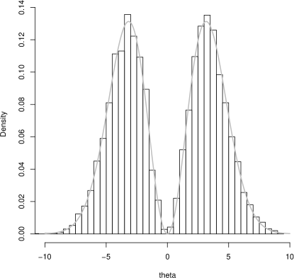
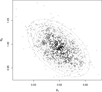
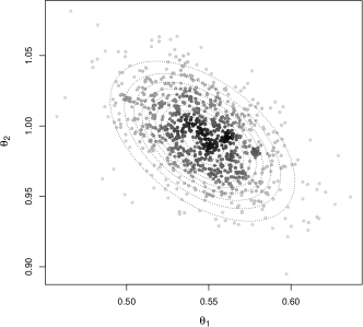
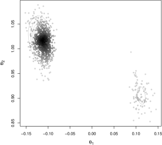
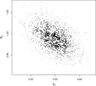
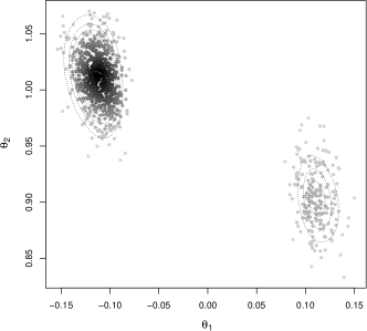
We simulate 1,000 realizations from , where are drawn from a bivariate Normal with , , . We first consider , , and compute posterior probabilities for the four possible models. We assign equal a priori probabilities and obtain exact integrated likelihoods using functions pmomMarginalU, pimomMarginalU and pemomMarginalU in the mombf package (the former is available in closed-form, for the latter two we used importance samples). The posterior probability assigned to the full model under all three priors is 1 (up to rounding) (Table 1). Figure 3 (left) shows 900 Gibbs draws (100 burn-in) obtained under the full model. The posterior mass is well-shifted away from 0 and resembles an elliptical shape for the three priors. Table 2 gives the first-order auto-correlations, which are very small. This example reflects the advantages of the orthogonalization strategy, which is particularly efficient as the latent truncation becomes negligible.
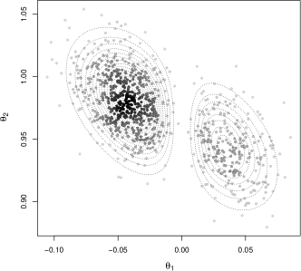
We now set , and keep and as before. We simulated several data sets and in most cases did not observe a noticeable posterior multi-modality. We portray a specific simulation that did exhibit multi-modality, as this poses a greater challenge from a sampling perspective. Table 1 shows that the data-generating model adequately concentrated the posterior mass. Although the full model was clearly dismissed in light of the data, as an exercise we drew from its posterior. Figure 3 (right) shows 900 Gibbs draws after a 100 burn-in, and Table 2 indicates the auto-correlation. The sampled values adequately captured the multiple modes.
5.2 High-dimensional estimation
 |
 |
 |
 |
 |
 |
| , | |
 |
 |
| , | |
 |
 |
| , | |
 |
 |
| , | |
 |
 |
| , | |
 |
 |
| , | |
 |
 |
We perform a simulation study with and growing dimensionality . We set for , the remaining 5 coefficients to and consider residual variances . Covariates were sampled from , where has unit variances and all pairwise correlations set to or . We remark that are population correlations, the maximum absolute sample correlations when being for (respectively), and , , when . We simulated 1,000 data sets under each setup.
Parameter estimates were obtained via BMA. Let be the model indicator. For each simulated data set, we performed 1,000 full Gibbs iterations (100 burn-in) which are equivalent to 1,000 birth-death moves. These provided posterior samples from . We estimated model probabilities from the proportion of MCMC visits and obtained posterior draws for using the algorithms in Section 4.2. For benchmark (BP) and hyper-g (HG) priors we used the same strategy for and drew from their corresponding posteriors.
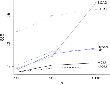
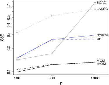
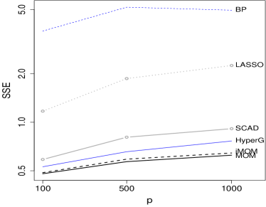
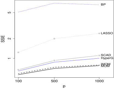
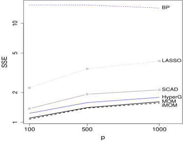
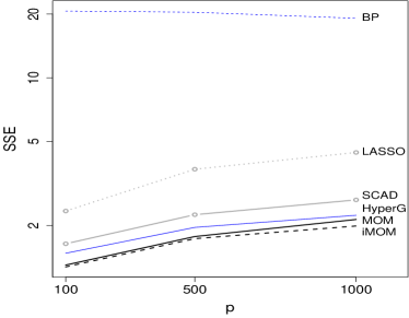
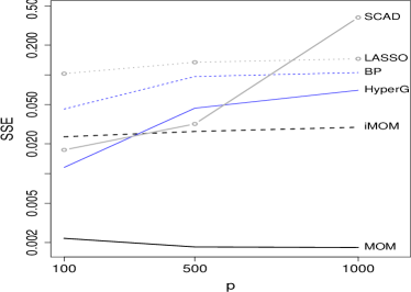
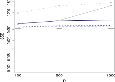
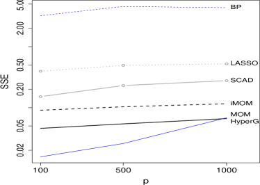
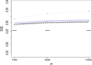
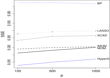
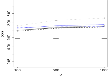
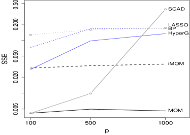
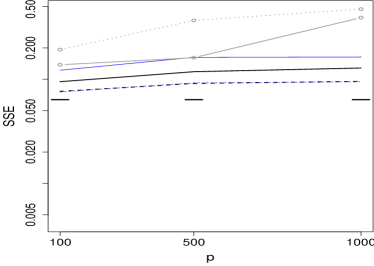
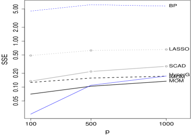
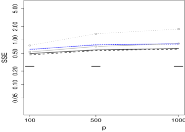
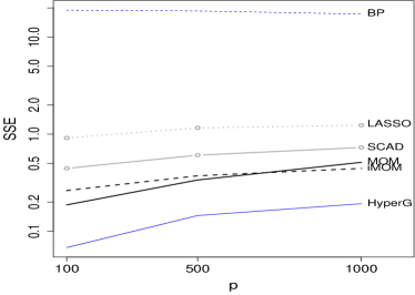
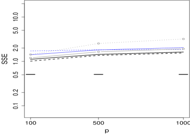
Figure 4 shows sum of squared errors (SSE) averaged across simulations for , . pMOM and piMOM perform similarly and present an SSE between 1.15 and 10 times lower than other methods in all scenarios. As grows, differences between methods tend to be larger. To obtain more insight on how the lower SSE is achieved, Figures 5-6 show SSE separately for (left) and (right). The largest differences between methods were observed for , where SSE remains very stable as grows for pMOM and piMOM. For differences in SSE are smaller, iMOM slightly outperforming MOM. Here SSE tends to be largest for LASSO. For all methods as signal-to-noise ratios decrease the SSE worsens relative to the least squares oracle estimator (Figures 5-6, right panels, black horizontal segments).
5.3 Gene expression data
| CPU time | |||||
|---|---|---|---|---|---|
| MOM | 4.3 | 0.566 | 6.5 | 0.617 | 1m 52s |
| iMOM | 5.3 | 0.560 | 10.3 | 0.620 | 59m |
| BP | 4.2 | 0.562 | 259.0 | 0.014 | 21h 27m |
| HG | 10.5 | 0.559 | 116.6 | 0.419 | 74 days |
| SCAD | 29 | 0.565 | 81 | 0.535 | 16.7s |
| LASSO | 42 | 0.586 | 159 | 0.570 | 23.7s |
We assess predictive performance in high-dimensional gene expression data. ? used mice experiments to identify 172 genes potentially related to the gene TGFB, and showed that these were related to colon cancer progression in an independent data set with human patients. TGFB plays a crucial role in colon cancer, hence it is important to understand its relation to other genes. Our goal is to predict TGFB in the human data, first using only the genes and then adding 10,000 extra genes. Both response and predictors were standardized to zero mean and unit variance (data in Supplementary Material). We assessed predictive performance via the leave-one-out cross-validated coefficient between predictions and observations. For Bayesian methods we report the posterior expected number of variables in the model (i.e. the mean number of predictors used by BMA), and for SCAD and LASSO the number of selected variables.
Table 3 shows the results. For all methods achieve similar , that for LASSO being slightly higher, although pMOM, piMOM and BP used substantially less predictors. These results appear reasonable in a moderately dimensional setting where genes are expected to be related to TGFB. However, when using predictors important differences between methods are observed. The BMA estimates based on MOM and iMOM priors remain parsimonious (6.5 and 10.3 predictors, respectively) and the cross-validated increases roughly by 0.05. In contrast, for the remaining methods the number of predictors increased sharply (the smallest being 81 predictors for SCAD) and a drop in was observed. Predictors with large marginal inclusion probabilities in MOM/iMOM included genes related to various cancer types (ESM1, GAS1, HIC1, CILP, ARL4C, PCGF2), TGFB regulators (FAM89B) or AOC3 which is used to alleviate certain cancer symptoms. These findings suggest that NLPs were extremely effective in detecting a parsimonious subset of predictors in this high-dimensional example. We also note that computation times were orders of magnitude lower than for LPs, pMOM being competitive with the penalized likelihood methods. Although run times depend on implementation issues, both BMS and mombf are coded in C and follow similar algorithms (e.g. storing marginal likelihoods in memory, updating one variable at a time). NLPs focus posterior mass on smaller models, which greatly alleviates the burden required for matrix inversions (non-linear cost in the model size). Further, NLPs tend to concentrate posterior probability on a smaller subset of models, which tend to be revisited and hence the marginal likelihood need not be recomputed. Regarding the efficiency of our proposed posterior sampler for , we ran 10 independent chains with 1,000 iterations each and obtained mean serial correlations of (pMOM) and (piMOM) across all non-zero coefficients. The mean correlation between across all chain pairs was (pMOM and piMOM).
6 Discussion
We showed how combining BMA with NLPs gives a coherent joint framework, encouraging parsimony in model selection and, for parameter estimation, selective shrinkage focused on spurious coefficients. Coupled with a theoretical investigation of NLP properties, we provide constructions based on truncation mixtures: to motivate NLPs from first principles, add flexibility in prior choice and facilitate posterior sampling, which we fully developed for linear regression. We obtained remarkable results when in simulations and gene expression data, with parsimonious models achieving accurate cross-validated predictions and good computation times. We did not require procedures to pre-screen covariates. Posterior samples a reasonable serial correlations, captured multi-modalities and independent runs delivered virtually identical estimates.
Our results show that it is not only possible to use the same prior for estimation and selection, but it may indeed be desirable. We remark that we used default informative priors, which are relatively popular for testing, but perhaps less readily adopted for estimation. Developing objective Bayes strategies to set the prior parameters is an interesting venue for future research, as well as determining shrinkage rates in more general cases, and adapting the latent truncation construction beyond linear regression, e.g. generalized linear, graphical or mixture models.
Appendix A Proofs and Miscellanea
A.1 Proof of Proposition 1
We start by stating two useful lemmas.
Lemma 1.
Let be either the pMOM, peMOM or piMOM prior, where as for any and is a local prior. Then , where for some constant and is a local prior.
Proof.
The result for the peMOM is direct with and . For the piMOM prior we multiply and divide the density by a Cauchy kernel, obtaining
| (13) |
where . By performing a change of variables we obtain the implied prior . Now, is continuous, has positive derivative for all and negative for , and , and hence . In summary, for the product eMOM and for the product iMOM, where .
The pMOM prior density has an unbounded term , but it can be rewritten as
| (14) |
for some , where it is straightforward to see that is now bounded. ∎
Lemma 2.
Let be a continuous and differentiable function satisfying for all . Define
where almost surely for any fixed , some set and a corresponding suitably defined -neighborhood . If for all then . Likewise, if for all and some then almost surely as . In particular, if is a singleton, then .
Proof.
Consider
| (15) | |||
where and the second term can be made arbitrarily small. Because is continuous, if for all then can also be made arbitrarily small a.s. as , and hence . Suppose now that for all , then from (15)
| (16) |
where due to continuity can be made arbitrarily close to for small enough and the integral on the right hand side of (16) can be made arbitrarily close to 1 as . The proof for when follows as an immediate implication. ∎
Proof of Proposition 1. Part (i) follows from direct algebraic manipulation
as desired. In a slight abuse of notation, in the derivation above and indicate integration with respect to the corresponding -finite dominating measures.
For Part (ii) we use Lemma 1, which states that the piMOM and peMOM priors can be written as with bounded , so that
| (17) |
where by assumption almost surely as for any and . See e.g. ? for such MLE consistency under general settings.We note that associated to either pMOM, piMOM or peMOM priors are products of independent Normal or Cauchy kernels assigning strictly positive density to any , which combined with MLE consistency guarantee that the limiting posterior concentrates arbitrarily large probability on any neighborhood of as (?). Part (ii) follows from Lemma 2. For the pMOM prior, from Lemma 1
| (18) |
where , is bounded and is the integrated likelihood under a prior. Part (ii) follows from Lemma 2, which guarantees convergence for the integral in (18), and that by assumption almost surely as . We note that from Bayes theorem
| (19) |
for any , where the second term in the right hand side is bounded (e.g. for ). The first term is the ratio of posterior densities under and , which for limiting normal posterior distributions with bounded covariance eigenvalues converges in probability to a bounded constant.
In the particular case where the data-generating density belongs to the set of considered models, i.e. for some . By definition of NLP we obtain that if and only if . Therefore, implies that and implies for some constant . We note that for non-identifiable models the set is no longer a singleton, but when by definition for all , hence we still obtain . Also by NLP definition, when then for all , which implies .
A.2 Proof of Proposition 2
We start by stating two lemmas.
Lemma 3.
Let be a linear model as in Proposition 2, and consider a NLP . Assume that the NLP penalty takes the product form , where is either the MOM penalty or for all and some constant , as in the eMOM or iMOM penalties. Then is a continuous function of .
Proof.
To prove the result for bounded penalties recall that is sufficient under and hence we may write
| (20) |
Now, letting and using the Dominated Convergence Theorem we obtain
| (21) |
and hence
| (22) |
showing that is continuous.
Consider now the MOM prior case. For the particular prior choice , ? showed that where , with and . ? gave explicit expressions for such products as a sum of continuous functions, and hence is continuous. Lemma 1 ensures that the pMOM penalty is also bounded for more general priors . Therefore,
| (23) |
where is the integrated likelihood with respect to and is the Normal posterior implied by the prior. Because for some constant , the Dominated Convergence Theorem gives that
| (24) |
so that direct algebraic manipulation after adding the integrated likelihood terms delivers
| (25) |
which proves that is continuous. ∎
Proof.
The proof runs analogous to that in Lemma 3, except that now the limit is taken with respect to and the term may grow as . That is, for bounded the argument proceeds by using the Dominated Convergence Theorem to obtain
| (28) |
so that
| (29) |
For the MOM prior we adjust the argument slightly. From (38) we obtain
| (30) |
where in (35) plugging in , . Following the same argument as in the proof of Lemma 3, we divide and multiply by a kernel to obtain
| (31) |
where for some constant , , , and . Now, because is bounded and the remaining expression in (31) is a probability density function on , the Dominated Convergence Theorem gives
| (32) |
which after rearranging terms gives
| (33) |
concluding the proof.
∎
We now proceed to prove Proposition 2.
For Part (1) we note that gives for fixed , which in turn guarantees (?). This implies , given that by assumption. Hence, . Since as and is assumed continuous, the Continuous Mapping Principle gives .
To show that , we note that is a one-to-one function with the sufficient statistic under . Hence is also sufficient and depends only on , so that we may write
| (34) |
where straightforward algebra shows that
| (35) |
where is the normalization constant for (which may depend on ) and that for the marginal posterior of .
Lemma 3 gives that is continuous in , hence by the Continuous Mapping Principle
| (36) |
where . For a fixed sequence of (36) is just a sequence in . To complete the proof we just need to show that for any sequence satisfying the theorem assumptions, which combined with would give that . By Lemma 4,
| (37) |
| (38) |
where IG denotes the inverse gamma density function.
Informally, given the assumptions on , for (38) to converge to a point mass at we need the trace of to converge to 0. Note that , which is satisfied as long as grows faster with than does, and that under our assumptions . Formally, the conditions on the eigenvalues of imply that for ,
| (39) |
We first study the second line in (39). Given that , for bounded we have for all the second line in (39) converges to 0 as for any given and all , i.e. converges to a point mass at .
Now suppose that is unbounded in a 0 Lebesgue measure set . In this case it also holds that
| (40) |
for any . This can be seen by contradiction, i.e. assume that for and an arbitrary small there exists some such that for some arbitrarily large values of . Then the prior probability of
| (41) |
but the integrand is positive and increasing with and hence by the Monotone Convergence Theorem (41) converges to as , which would imply that is improper.
A.3 Proof of Proposition 3, Part (i)
For ease of notation we drop the subindex indicating the model and we denote . Consider first the pMOM prior and take without loss of generality. The log-posterior density is
| (42) |
where is the log-likelihood and is the prior density on . Suppose that the sampling model satisfies the conditions in ?, then can be approximated by a second order Taylor expansion around an MLE of . Performing this expansion and setting the partial derivative with respect to to 0 delivers
| (43) |
where is the element of the Hessian of evaluated at . Rearranging terms we obtain
| (44) |
We note that the Taylor approximation to (42) is a quadratic form in , which is convex in , plus which is convex in each quadrant of (i.e. for fixed sign of ) and converges to as any . Therefore the function to maximize has a global maxima at the quadrant where occurs and a local maxima in each other quadrant. Consider first the two modes for occurring when for . Under Walker’s conditions , with finite (condition B4), and , where minimizes KL divergence to the data-generating model and we assume that . Incorporating these facts into (44) gives that any posterior mode must satisfy
| (45) |
with . We note that (45) remains valid for linear models with bounded eigenvalues as stated in the proposition assumptions, given that then is exactly quadratic and the condition ensures almost sure convergence of the MLE, which implies and . Now suppose that , then for one mode and thus , whereas solving (45 gives that the other mode . Next assume that , then and hence . This implies that , which from (45) implies that with . To summarize, the modes when for are either from the MLE or from 0. All other modes are given by the intersection of the contours of an ellipse centered at and all axis lengths shrinking at rate (from boundedness of eigenvalues) with the isocontours for some (which do not depend on ). Hence all modes occurring at quadrants other than that of shrink towards 0 at the same rate, i.e. .
The proof for the piMOM and peMOM priors follows in an analogous fashion. Performing a second order Taylor approximation to the piMOM posterior around an MLE and setting the partial derivative with respect to to 0 delivers that and must satisfy
| (46) |
where as before indicates the Hessian of evaluated at . Rearranging terms delivers
| (47) |
We again consider the modes for when for . Either Walker’s conditions for general models or the eigenvalue conditions in the linear model case guarantee that for all , whereas MLE consistency gives that , and . Therefore, must satisfy
| (48) |
where . Consider the case where the true parameter value , then for one mode and hence with , whereas from 48 the other mode . Now consider the case when , then and hence with . Similarly to the pMOM proof, all axes corresponding to the quadratic expansion contract exactly at rate , hence all other modes . The proof for the peMOM case proceeds identically, with the only difference that term in (47) changes for , hence one obtains the same convergence in probability for .
A.4 Proof of Proposition 3, Part (ii)
We first state a lemma regarding the derivatives of the univariate log-MOM, eMOM and iMOM prior densities with prior dispersion . The do not prove the lemma, as it follows from straightforward algebra.
Lemma 5.
Let .
-
(i)
Let be the MOM density, then
-
(ii)
Let be the eMOM density, then
-
(iii)
Let be the eMOM density, then
A.5 Proof of Proposition 3, Part (ii)
Consider Proposition 3(ii) for general models that satisfy the conditions in ?. For ease of notation we drop the subindex and conditioning on model . The posterior expectation of interest is
| (49) |
where is the log-likelihood function. We shall use Theorem 4 in ? to obtain a Laplace approximation to (49) by expanding around its main posterior mode . We note that when the true parameter value the posterior multi-modality does not vanish even as , but defer discussion of this point to later in the proof. We note that Walker’s conditions ensure that the model is Laplace regular and hence Theorem 4 in ? can be used. To use the theorem we set , and and note that are four times and six times differentiable. We also note that when is either the eMOM or iMOM prior density, it is infinitely differentiable but not analytical at , but cannot occur at 0 (the prior density is 0) and hence we may ignore this set with 0 Lebesgue measure. Direct application of Theorem 4 in ? gives
| (50) |
where , denotes the element of the Hessian of evaluated at , that of the inverse Hessian and are third derivatives. That is,
| (51) |
From the Normal approximation to the likelihood we obtain that unless , in which case . Hence,
| (52) |
Walker’s conditions ensure that for converge in probability to a finite . Regarding , the first term converges to whereas the second term is when and when for either the MOM, eMOM or iMOM prior (Proposition 3(i) and Lemma 5), hence . This in turn implies that the Hessian converges in probability to plus diagonal terms that either converge to 0 or are , and hence the elements in its inverse . Finally consider . From Lemma 5 when we obtain for either the MOM, eMOM or iMOM priors. When for the MOM prior for and for . For the eMOM and iMOM priors for and again for . Therefore, from (50) we obtain that if for and if for any . In particular, in cases of parameter orthogonality where for all then the difference between the posterior mean and posterior mode of is whenever . To conclude the proof, we recall that the posterior is multi-modal and hence approximate by adding (50) across the modes. Proposition 3 that for such modes for pMOM and for peMOM and piMOM, hence for MOM and for eMOM or iMOM.
A.6 Proof of Proposition 3, Part (iii)
We consider linear models of growing dimensionality, again dropping the model subindex for ease of notation. Although we assume that is a diagonal matrix, we state part of the argument for general (subject to the eigenvalue conditions in Proposition 2) and make explicit where the orthogonality assumption is needed. As argued during the proof of Proposition 3(i), the rates for posterior modes remain valid for linear models with such bounded eigenvalues. Regarding the posterior mean, the assumed conditions on the eigenvalues of guarantee Laplace regularity (?) and hence the expansion (50) remains valid, where now
| (53) |
Therefore is given by the element in for , , which is . For we add , which from Lemma 5 and Proposition 3 is for and for (for pMOM, peMOM and piMOM), hence . The elements are given by the vector
| (54) |
where contains for . Given that the eigenvalues of are bounded the first term in (54) converges in probability to 0 for the main mode and is for all other modes. From Lemma 5 and Proposition 3(i) it is straightforward to see that , hence for . Similarly,
| (55) |
Regarding the elements in the inverse Hessian , the Hessian is positive definite with and hence for .
Finally we obtain third derivatives . Because is given by the corresponding element , for . For , for the main mode under either a pMOM, peMOM or piMOM prior (Lemma 5), whereas for other modes under a pMOM or under a peMOM or piMOM priors (Proposition 3(i)). From (50), the contribution to from each mode is
| (56) |
plus a lower order term.
Consider now that is orthogonal. In that case for and the two values maximizing the posterior are independent of for . Therefore under a pMOM prior
| (57) |
whereas
| (58) |
under either a peMOM or piMOM prior, which concludes the proof.
A.7 Proof of Proposition 4, Part (i)
Consider models for , all satisfying the conditions in ?. Let be the true model and let be such that . Consider first the pMOM prior. The marginal likelihood under can be approximated by a Laplace expansion around each posterior mode for , so that
| (59) |
where is the log-likelihood and the Hessian of the log-likelihood plus the log-prior density evaluated at . Expressions for the elements in are given in the proof of Proposition 3 for pMOM, peMOM and piMOM priors.
Without loss of generality denote by the mode located in the same quadrant as the MLE . As seen in Proposition 3, under Walker’s conditions and for a positive-definite , hence (59) converges in probability to
| (60) |
where . For modes in any other quadrant , where is the Kullback-Leibler divergence between the data-generating model and that where some elements in are set to 0 (which is positive by assumption). Further, in such quadrants so that the sum of (59) across all modes gives that the marginal likelihood
| (61) |
where for .
Now consider such that . Denote by the subset of such that and that for , where minimizes Kullback-Leibler divergence to the data-generating model, which under our assumptions is and hence . Following the same argument as for , it suffices to focus on modes for which lies in the same quadrant as . Adding up the Laplace approximations across all such modes delivers the Bayes factor
| (62) |
where the first term is , the second term converges in probability to for some random variable , the third and fourth terms converge in probability to a positive constant ( is bounded by assumption). Therefore each summand in (62) is , and given that we are adding up a finite number of terms . Next consider such that . By assumption, the minimum Kullback-Leibler divergence between and any with is strictly positive. Hence by the law of large numbers and .
The proof for the peMOM and piMOM are largely analogous. The marginal likelihood for is
| (63) |
where for the peMOM under any model, whereas for the piMOM under and under any other , and consequently . Consider such that , then from Proposition 3(i) for all modes with in the same quadrant as we have , where . Thus the Bayes factor
| (64) |
The proof for the case proceeds in the same manner as for the pMOM.
A.8 Proof of Proposition 4, Part (ii)
We start by using the Bayes factor rates proven in Part (i) to derive rates for posterior model probabilities. Consider a model such that and note that . Under a pMOM prior
| (65) |
where the last equality follow from the assumption that and hence the denominator is . The same argument applies under a peMOM or piMOM prior, where now and hence . Finally, for models such that , from Proposition 4(i) .
The BMA posterior mean is
| (66) |
Suppose first that . From Proposition 3(ii), for pMOM, peMOM and piMOM, where is the MLE. Also, in the second term of (66) is and is either (pMOM) or (peMOM, piMOM). Further, by assumption and hence the whole second term in (66) is . Regarding the third term in (66), and . Summarizing, when for the pMOM we have that
| (67) |
and for the peMOM or piMOM
| (68) |
Now consider the case . Obviously, only includes non-zero coefficients and hence . In the second term of (66), from Proposition 3(ii) we have that is for pMOM and for peMOM and piMOM. Thus the whole second term is for pMOM and for peMOM and piMOM, where for . As in the case, the third term is . Summarizing, when we obtain
| (69) |
and for the peMOM or piMOM
| (70) |
as desired.
A.9 Proof of Proposition 4, Part (iii)
We adjust the notation of the previous sections slightly to ease the upcoming exposition. Let for (where ) be the coefficient corresponding to variable , and let be variable inclusion indicators. We aim to characterize . We first derive . Let and be the result from removing from , and note that . Denote by , because is orthogonal the likelihood factors across , and given that the pMOM, peMOM and piMOM priors also factors straightforward algebra shows that
| (71) |
where
| (72) |
For the pMOM prior , and , for the peMOM prior and again , , and for the piMOM prior , , . The assumption that are exchangeable a priori is equivalent to stating that for a certain hyper-parameter , and hence
| (73) |
Denoting by the prior density of ,
| (74) |
and hence
| (75) |
Following the same argument as in Proposition 4(ii), if then under either a pMOM, peMOM or piMOM prior. If then for pMOM and for peMOM and piMOM.
We now characterize . Again, because of orthogonality this posterior mean is the same under any model with , giving
| (76) |
As before for the pMOM prior and hence by using Normal moments of up to order 3 (76) becomes , where and . For the peMOM and piMOM, using a Laplace approximation (?) around the two modes as in Proposition 3 gives that if then (where is the MLE) and if then .
Combining the rates derived above for and , if then for pMOM, peMOM and piMOM, whereas if then for pMOM and for peMOM and piMOM.
A.10 Proof of Proposition 5
The goal is to show that for all there exists such that implies . By construction, the conditional prior density is , where . Let be a value such that , and express the prior density as
| (77) |
The second term in (77) is 0, as by assumption . Now, consider that for , is minimized at , and therefore (77) can be bounded by
| (78) |
Notice that the numerator can be made arbitrarily small by decreasing , since is bounded around , by assumption there is no prior mass at so that the cdf in the numerator converges to 0 as , and that denominator converges to 1 as . That is, it is possible to choose such that , which gives the result. ∎
A.11 Proof of Corollary 1
Replace by in the proof of Proposition 5. Letting any go to 0 and applying the same argument delivers the result.
A.12 Proof of Proposition 6
We first note that in order for to be proper the random variable must have finite expectation with respect to . Now, the marginal prior for is
| (79) |
Suppose we set , which we can do as long as . Then , which proves the result. The only step left is to show that indeed . In general
| (80) |
where is the survival function of the positive random variable and therefore (80) is equal to its expectation with respect to , which is finite as discussed at the beginning of the proof. ∎
A.13 Proof of Corollary 2
A.14 Proof of Proposition 7
By definition, the marginal density
| (82) |
where is the cdf of evaluated at . As we have that converges to a point mass at zero and hence the integral in the right hand side of (82) converges to . To finish the proof of (i) notice that for some by the Mean Value Theorem, as long as is differentiable and continuous at , i.e. is a continuous random variable. In the particular case , note that is continuous and .
To prove (ii) notice that as and that the integral in the right hand side of (82) is , which is increasing with as is monotone decreasing in . Hence, where increases as . Furthermore, if the Monotone Converge Theorem applies and converges to a finite constant. ∎
A.15 Proof of Corollary 3
Because have independent marginals,
| (83) |
where is a multivariate survival function and decreases as . Hence as decreases. To find the limit as we note that the integral is bounded by the finite integral obtained plugging into the integrand. Hence, the Dominated Convergence Theorem applies and and from (83) . Since are continuous the Mean Value Theorem applies, so that for some . To prove (ii), notice that as and that increases as . Hence, where increases with , which proves (ii). Further, if the Monotone Convergence Theorem applies and for finite . ∎
A.16 Multivariate Normal sampling under outer rectangular truncation
The goal is to sample with truncation region . We generalize the Gibbs sampling of ? and importance sampling of ? and ? to the non-convex region .
Let be the Cholesky decomposition of and its inverse, so that is the identity matrix, and define . The random variable follows a distribution with truncation region . Since , denoting as the row in we obtain the truncation region .
The full conditionals for given needed for Gibbs sampling follow from straightforward algebra. Denote by the element in , then truncated so that either or hold simultaneously for . We now adapt the algorithm to address the fact that this truncation region is non-convex.
The region excluded from sampling can be written as , when and when (analogously for ). as given is the union of possibly non-disjoint intervals, which complicates sampling. Fortunately, it can be expressed as a union of disjoint intervals with the following algorithm. Suppose that are sorted increasingly, set , and . For repeat the following two steps.
-
1.
If set , and , else if and set .
-
2.
Set .
Finally, because are disjoint and increasing, we may draw a uniform number in excluding intervals and set , where is the inverse Normal cdf.
A.17 Monotonicity and inverse of iMOM prior penalty
Consider the product iMOM prior as given in (9). We first study the monotonicity of the penalty , which for simplicity here we denote as , and then provide an algorithm to evaluate its inverse function. Equivalently, it is convenient to consider the log-penalty
| (84) |
as its inverse uniquely determines the inverse of . Denoting , (84) can be written as
| (85) |
To show the monotonicity of (85) we compute its derivative and show that it is positive for all . Clearly, both when and we have positive . Hence we just need to see that there is some for which all roots of are imaginary, so that for all . Simple algebra shows that the roots of are , so that for there are no real roots. Hence, for is monotone increasing.
We now provide an algorithm to evaluate the inverse. That is, given a threshold we seek such that . Our strategy is to obtain an initial guess from an approximation to and then use continuity and monotonicity to bound the desired and conduct a linear interpolation based search. Inspecting the expression for in (85) we see that the term is dominated by when approaches 0 and by when is large. Hence, we approximate by dropping the term, obtaining
| (86) |
Setting (86) equal to and solving for gives as an initial guess, where .
If we set a lower bound and an upper bound obtained by increasing by a factor of 2 until . Similarly, if we set the upper bound and find a lower bound by successively dividing by a factor of 0.5. Once are determined, we use a linear interpolation to update , evaluate and update either or . The process continues until is below some tolerance (we used ). In our experience the initial guess is often quite good and the algorithm converges in very few iterations.
Acknowledgments
This research was partially funded by the NIH grant R01 CA158113-01.
References
- [1]
- [2] [] Bayarri, M., & Garcia-Donato, G. (2007), “Extending conventional priors for testing general hypotheses in linear models,” Biometrika, 94, 135–152.
- [3]
- [4] [] Bhattacharya, A., Pati, D., Pillai, N., & Dunson, D. (2012), Bayesian shrinkage,, Technical report, arXiv preprint arXiv:1212.6088.
- [5]
- [6] [] Calon, A., Espinet, E., Palomo-Ponce, S., Tauriello, D., Iglesias, M., Céspedes, M., Sevillano, M., Nadal, C., Jung, P., Zhang, X.-F., Byrom, D., Riera, A., Rossell, D., Mangues, R., Massague, J., Sancho, E., & Batlle, E. (2012), “Dependency of colorectal cancer on a TGF-beta-driven programme in stromal cells for metastasis initiation,” Cancer Cell, 22(5), 571–584.
- [7]
- [8] [] Castillo, I., Schmidt-Hieber, J., & van der Vaart, A. (2014), Bayesian linear regression with sparse priors,, Technical report, arXiv preprint arXiv:1403.0735.
- [9]
- [10] [] Castillo, I., & Van der Vaart, A. W. (2012), “Needles and Straw in a Haystack: Posterior Concentration for Possibly Sparse Sequences,” The Annals of Statistics, 40(4), 2069–2101.
- [11]
- [12] [] Consonni, G., & La Rocca, L. (2010), On Moment Priors for Bayesian Model Choice with Applications to Directed Acyclic Graphs,, in Bayesian Statistics 9 - Proceedings of the ninth Valencia international meeting, eds. J. Bernardo, M. Bayarri, J. Berger, A. Dawid, D. Heckerman, A. Smith, & M. West, Oxford University Press, pp. 119–144.
- [13]
- [14] [] Dawid, A. (1999), The trouble with Bayes factors,, Technical report, University College London.
- [15]
- [16] [] Fan, J., & Li, R. (2001), “Variable selection via nonconcave penalized likelihood and its oracle properties,” Journal of the American Statistical Association, 96, 1348–1360.
- [17]
- [18] [] Fan, J., & Lv, J. (2010), “A selective overview of variable selection in high dimensional feature space,” Statistica Sinica, 20, 101–140.
- [19]
- [20] [] Fernández, C., Ley, E., & Steel, M. (2001), “Benchmark priors for Bayesian model averaging,” Journal of Econometrics, 100, 381–427.
- [21]
- [22] [] Gelfand, A., & Ghosh, S. (1998), “Model choice: A minimum posterior predictive loss approach,” Biometrika, 85, 1–11.
- [23]
- [24] [] Ghosal, S. (2002), A review of consistency and convergence of posterior distribution,, Technical report, Indian Statistical Institute.
- [25]
- [26] [] Hajivassiliou, V. (1993), “Simulating normal rectangle probabilities and their derivatives: the effects of vectorization,” Econometrics, 11, 519–543.
- [27]
- [28] [] Jeffreys, H. (1961), Theory of Probability, third edn, Oxford, England: Oxford University Press.
- [29]
- [30] [] Johnson, V., & Rossell, D. (2010), “Prior Densities for Default Bayesian Hypothesis Tests,” Journal of the Royal Statistical Society B, 72, 143–170.
- [31]
- [32] [] Johnson, V., & Rossell, D. (2012), “Bayesian model selection in high-dimensional settings,” Journal of the American Statistical Association, 24(498), 649–660.
- [33]
- [34] [] Kan, R. (2008), “From moments of sum to moments of product,” Journal of Multivariate Analalysis, 99, 542–554.
- [35]
- [36] [] Kass, R., Tierney, L., & Kadane, J. (1990), “The validity of posterior expansions based on Laplace’s method,”.
- [37]
- [38] [] Kass, R., & Wasserman, L. (1995), “A reference Bayesian test for nested hypotheses and its relationship to the Schwarz criterion,” Journal of the American Statistical Association, 90, 928–934.
- [39]
- [40] [] Keane, M. (1993), “Simulation estimation for panel data models with limited dependent variables,” Econometrics, 11, 545–571.
- [41]
- [42] [] Klugkist, I., & Hoijtink, H. (2007), “The Bayes factor for inequality and about equality constrained models,” Computational Statistics & Data Analysis, 51(12), 6367 – 6379.
- [43]
- [44] [] Kotecha, J., & Djuric, P. (1999), Gibbs sampling approach for generation of truncated multivariate Gaussian random variables,, in Proceedings, 1999 IEEE International Conference on Acoustics, Speech and Signal Processing, IEEE Computer Society, pp. 1757–1760.
- [45]
- [46] [] Lai, T., Robbins, H., & Wei, C. (1979), “Strong consistency of least squares in multiple regression,” Journal of multivariate analysis, 9, 343–361.
- [47]
- [48] [] Liang, F., Paulo, R., Molina, G., Clyde, M., & Berger, J. (2008), “Mixtures of g-priors for Bayesian Variable Selection,” Journal of the American Statistical Association, 103, 410–423.
- [49]
- [50] [] Liang, F., Song, Q., & Yu, K. (2013), “Bayesian modeling for high-dimensional generalized linear models,” Journal of the American Statistical Association, 108(502), 589–606.
- [51]
- [52] [] Martin, R., & Walker, S. (2013), Asymptotically minimax empirical Bayes estimation of a sparse normal mean vector,, Technical report, arXiv preprint arXiv:1304.7366.
- [53]
- [54] [] Moreno, E., Bertolino, F., & Racugno, W. (1998), “An intrinsic limiting procedure for model selection and hypotheses testing,” Journal of the American Statistical Association, 93, 1451–1460.
- [55]
- [56] [] Narisetty, N., & He, X. (2014), “Bayesian variable selection with shrinking and diffusing priors,” The Annals of Statistics, 42(2), 789–817.
- [57]
- [58] [] O’Hagan, A. (1995), “Fractional Bayes factors for model comparison,” Journal of the Royal Statistical Society, Series B, 57, 99–118.
- [59]
- [60] [] Pérez, J., & Berger, J. (2002), “Expected posterior prior distributions for model selection,” Biometrika, 89, 491–512.
- [61]
- [62] [] Redner, R. (1981), “Note on the consistency of the maximum likelihood estimator for nonidentifiable distributions,” Annals of Statistics, 9(1), 225–228.
- [63]
- [64] [] Rodriguez-Yam, G., Davis, R., & Scharf, L. (2004), Efficient Gibbs sampling of truncated multivariate normal with application to constrained linear regression, PhD thesis, Department of Statistics, Colorado State University.
- [65]
- [66] [] Rossell, D., Telesca, D., & Johnson, V. (2013), High-dimensional Bayesian classifiers using non-local priors,, in Statistical Models for Data Analysis XV, Springer, pp. 305–314.
- [67]
- [68] [] Rousseau, J. (2007), Approximating interval hypothesis: p-values and Bayes factors,, in Bayesian Statistics 8, eds. J. Bernardo, M. Bayarri, J. Berger, & A. Dawid, Oxford University Press, pp. 417–452.
- [69]
- [70] [] Springer, M., & Thompson, W. (1970), “The distribution of products of Beta, Gamma and Gaussian random variables,” SIAM Journal of Applied Mathematics, 18(4), 721–737.
- [71]
- [72] [] Tibshirani, R. (1996), “Regression shrinkage and selection via the Lasso,” Journal of the Royal Statistical Society, B, 58, 267–288.
- [73]
- [74] [] Verdinelli, I., & Wasserman, L. (1996), Bayes factors, nuisance parameters and imprecise tests,, in Bayesian Statistics 5, eds. J. Bernardo, J. Berger, A. Dawid, & A. Smith, Oxford University Press, pp. 765–771.
- [75]
- [76] [] Walker, A. (1969), “On the asymptotic behaviour of posterior distributions,” Jornal of the Royal Statistical Society B, 31(1), 80–88.
- [77]
- [78] [] Wilhelm, S., & Manjunath, B. (2010), “tmvtnorm: a package for the truncated multivariate normal distribution,” The R Journal, 2, 25–29.
- [79]
- [80] [] Zellner, A., & Siow, A. (1984), Basic issues in econometrics, Chicago: University of Chicago Press.
- [81]