Bilateral symmetry and modified Pascal triangles
in Parsimonious games

Abstract

We discuss the prominent role played by bilateral symmetry and modified Pascal triangles in self twin games, a subset of constant sum homogeneous weighted majority games. We show that bilateral symmetry of the free representations unequivocally identifies and characterizes this class of games and that modified Pascal triangles describe their cardinality for combinations of $m$ and $k$, respectively linked through linear transforms to the key parameters $n$, number of players and $h$, number of types in the game.

Besides, we derive the whole set of self twin games in the form of a genealogical tree obtained through a simple constructive procedure in which each game of a generation, corresponding to a given value of $m$, is able to give birth to one child or two children (depending on the parity of $m$), self twin games of the next generation. The breeding rules are, given the parity of $m$, invariant through generations and quite simple.

Keywords

Homogeneous weighted majority games; bilateral symmetry; modified Pascal triangles; games representations.

^a Dept. of Economics and Statistics D.I.E.S., Udine University, Italy
^b Imperial College London, UK
^c Dept. of Economics and Statistics D.I.E.S., Udine University, Italy

1 Introduction

Bilateral Symmetry ($BS$) and Modified Pascal Triangles ($MPT$) are issues that play a significant role in various fields of sciences. Just to recall some of the most important papers on these subjects let us quote, for $BS$, the milestone book of Weyl ([19], 1952) and the papers by Gardner ([6], 1971), Møller and Thornill ([10], 1998), Finnerty ([5], 2003), Song et al ([16], 2010), Palmer ([12], 2004), and for $MPT$, Ando ([1], 1988), Granville ([7], 1992), Barry ([2], 2006), Trzaska ([17], 1991) and Bollinger ([3], 1993).

In this paper we will see that both issues jointly emerge in a game theory framework: precisely, as a key to self twin “parsimonious” games, a class of games introduced by Isbell ([9], 1956) in the early stage of game theory, which at the best of our knowledge did not receive then any attention.

Parsimonious games (hereafter $P$ games) are the subset of constant sum homogeneous weighted majority games characterized by the “parsimony property” to have, for any number $n$ of non dummy players in the game, the smallest number (i.e. exactly $n$) of minimal winning coalitions.

For such games the incidence matrix $M$ is the binary square $n\times n$ matrix whose entries are 1 (or 0) if column player $i$ belongs (does not belong) to the row minimal winning coalition $j$. A twin (dual) relationship on $P$ games has been introduced by Isbell ([9], p. 185) through the following property of their incidence matrices: the transposed ${M}^{T}$ of the incidence matrix ${M}$ of any $P$ game ${G}$ is the incidence matrix ${\overline{M}}$ of a $P$ game ${\overline{G}}$ called the twin of ${G}$.

${G}$ is self twin (self dual) if ${\overline{G}}$ is identical to ${G}$. We denote by $STP$ the set of self twin $P$ games.

Our starting point is that an alternative and more friendly description of the twin relationship may be obtained making recourse to a specific property of the vectorial representations of $P$ games.

Usually constant sum homogeneous weighted majority games, including $P$ games, are described by their classical minimal homogeneous representation $(q;{\bf w})$ where ${\bf w}=\{w_{1},w_{2},\ldots,w_{n}\}$ is the ordered $(w_{1}=1,w_{i}\leq w_{i+1}$ for any $i$) vector of individual minimal homogeneous integer weights and $q$ the minimal winning quota given by $q={1+\sum_{i\in N}w_{i}\over 2}$ and satisfying $q=\sum_{i\in S}w_{i}$, for any coalition $S$ of the so called minimal winning set.

As shown in sect. 2.2, alternative unequivocal representations of a $P$ game may be given either through its binary representation or through its type representation. In particular, the binary representation is the ordered $n$ dimensional vector ${\bf b}$ with components $b_{i}=1$ if $w_{i}>w_{i-1}$, $b_{i}=0$ otherwise $(w_{i}=w_{i-1})$. Note that the condition $w_{0}=0$, which gives zero weight to the fictitious player ($i=0$) representing the set of dummies, implies $b_{1}=1$. The type representation is the ordered $h$ $(2\leq h\leq n-2)$ dimensional vector ${\bf x}=(x_{1},x_{2},\ldots,x_{h})$ whose component $x_{t}$ is the number of players of type $t$ (sharing the same common type weight $w_{t}>w_{t-1}$) in the game.

Yet, some of the information embedded in such representations is redundant; indeed, the first two and the last two components of ${\bf b}$, like the last component of ${\bf x}$, are the same in any $P$ game. Then, what really matters in a $P$ game is the, $n-4$ dimensional, free binary representation ${}_{f}{\bf b}=(b_{3},\ldots,b_{n-3})$, or respectively the, $h-1$ dimensional, free type representation ${}_{f}{\bf x}=(x_{1},x_{2},\ldots,x_{h-1})$.

In terms of these free representations, $STP$ games are (as shown in Pressacco-Plazzotta, 2013, [13], sect. 4.2, p. 9) the subset of $P$ games characterized by bilateral symmetry. Exploiting bilateral symmetry it is straightforward to obtain closed form formulae for the cardinality of $STP$ games for feasible combinations of $(n,h)$ and to show that a properly $MPT$, $\Gamma$, with entries $\Gamma(m,k)$, describes the cardinality of $STP$ games with $n=m+4$ players and $h=k+2$ types.

Indeed we will show that the rule which governs the evolution with $m$ of the $MPT$ mimics the one holding in the classical Pascal triangle (i.e. the “Pascal equation”), except for internal entries corresponding to combinations of even $m$ and odd $k$. In detail, for such combinations is it $\Gamma(m,k)=\Gamma(m-1,k)-\Gamma(m-1,k-1)$, so as the difference rather than the sum of the adjacent entries of the previous row is to be computed (obviously this modification has a feedback on the whole triangle).

On the way we describe also the regularities of other related $MPT$: $\Delta$, which describes the cardinality (still as a function of the couple $m,k$) of the $P$ non self twin games, and $\Theta=\Delta/2$ the cardinality of couples of (non identical) twins.

Besides these counting results, we found also that the whole set of $STP$ may be described in the form of a genealogical tree, derived through a constructive procedure. In this approach successive generations of $STP$ are associated to the sequence of $m$ values, and each game may be seen as a parent which gives birth to one child or two children (depending on the even or odd character of the parent generation), $STP$ games of the next generation. The breeding rules, defined in terms of the free type representation, are simple and generations invariant, albeit parity specific.

A key role in the evolution of the genealogical tree is played by the pivot components of the subset of $STP$ games, whose ${}_{f}{\bf x}$ representation has an odd number of components (shortly OSTP games). We show that the structure of the pivot’s set is described by other “regular” triangles.

The plan of the paper is as follows. Section 2 recalls basic concepts of majority games, resumes relevant results on $P$ games and introduces the alternative binary and type representations, which play a key role in the subsequent sections. Section 3 is devoted to define bilateral symmetry seen as a particular aspect of the symmetry (or twin) relationship on $P$ games. In Section 4 closed form expressions of the number of $STP$ games for different feasible combinations of the parameters $n,h$ or $m,k$ are obtained. Section 5, the core of the paper, suggests and discusses an interpretation in terms of $MPT$ of such formulas. In Section 6 we build a genealogical tree of $STP$ games, through the application of simple evolutionary rules that may be translated in high speed algorithms. Section 7 introduces the pivot triangles and give results on their main evolutionary properties. Section 8 gives some examples and conclusions follow in Section 9.

2 Definitions and main results on $P$ games

2.1 Basics of weighted majority games

As usual $N=(1,\ldots,n)$ denotes the set of all (non dummy) players.

Definition 2.1.

A coalition $S$ is a subset of the set $N$. A game $G$ in coalitional function form is defined by the coalitional function of the game, that is the real function $v:\mathcal{P}(N)\rightarrow\mathbb{R}$.

Definition 2.2.

A game in coalitional function form is simple if its $v$ function has values in $\{0,1\}$. A coalition $S$ is winning if $v(S)=1$, losing if $v(S)=0$.

Definition 2.3.

A simple game is constant sum if, for any $S\in\mathcal{P}(N)$, $v(S)+v(\mathaccent 869{S})=1$.

Definition 2.4.

A coalition $S$ is said to be minimal winning if $v(S)=1$ and, for any $T\mathchar 13600\relax S$, $v(T)=0$. The set of minimal winning coalitions is denoted by $WM$. A player $i$ who does not belong to any minimal winning coalition is said dummy; at the other extreme, it is a dictator if it is $v(i)=1$. We will consider games free of dictator and dummies.

Definition 2.5.

A simple, weighted majority game is described by a representation $(q;{\bf w})$ where ${\bf w}$ is a vector $(w_{1},w_{2},\ldots,w_{n})$ of positive weights, $q>{1\over 2}\cdot w(N)={1\over 2}\cdot\sum_{i\in N}w_{i}$ is the winning quota and $v(S)=1\Leftrightarrow w(S)=\sum_{i\in S}w_{i}\geq q$.

Definition 2.6.

A representation $(q;{\bf w})$ of a weighted majority game is homogeneous if $w(S)=q$ for any $S$ of $WM$.

Definition 2.7.

Homogeneous weighted majority games are games for which (at least) a homogeneous representation exists.

Consider now the class of all simple, constant sum $n$ person homogeneous weighted majority games.

Result 2.1.

All games of such a class admit a minimal homogeneous representation, that is a (homogeneous) representation $(q;{\bf w})$ such that all weights are integers, there are players with (minimum) weight 1 and $q={w(N)+1\over 2}$, which implies for any $S\in WM$, $w(S)-w(\mathaccent 869{S})=1$.

Remark 2.1.

Hereafter we will suppose that in such a representation the vector ${\bf w}$ is ordered according to the convention $w_{1}=1,w_{i}\leq w_{i+1}$ for any $i$.

Result 2.2.

The cardinality of the $WM$ set of our class may be either greater or equal (but not lower) than $n$. See [9], p. 185.

2.2 Parsimoniuos games and their alternative representations

Definition 2.8.

We call Parsimoniuos games (hereafter $P$ games) the subset of constant sum homogeneous weighted majority games characterized by the parsimony property to have for any given number $n$ of non dummy players in the game the smallest number, i.e. exactly $n$, of minimal winning coalitions.

The nice properties of this class of games have been studied in a ground breaking paper (Isbell, 1956, [9]) going back to the early stage of game theory development. In particular, there it has been found that a $P$ game is univocally described also by an alternative binary representation.

Definition 2.9.

Given a $P$ game $G$ with minimal homogeneous representation $(q;{\bf w})$, its binary representation is the ordered (according to the non decreasing weight labelling) $n$ dimensional vector ${\bf b}$ with components: $b_{1}=1$ and for $i=2,\ldots,n$, $b_{i}=1$ if $w_{i}>w_{i-1}$, $b_{i}=0$ otherwise, i.e if $w_{i}=w_{i-1}$.

Result 2.3.

The following constraints ([9], p. 185) hold, in any $P$ game, on the first two and on the last two components of ${\bf b}$: $b_{1}=1$, $b_{2}=0$, $b_{n-1}=0$, $b_{n}=1$. Apart from these constraints, the choice of the other components of the binary representation is fully free.

Definition 2.10.

The free binary representation of a $P$ game with binary representation ${\bf b}$ is the ordered $n-4$ dimensional vector of the internal components of ${\bf b}$. We denote such a vector by ${}_{f}{\bf b}=(b_{3},\ldots,b_{n-2})$.

Result 2.4.

There is a one-to-one correspondence between the set of all feasible choices of ${}_{f}{\bf b}$ and the set of $P$ games; hence, putting (for any $n>3$) $m=n-4$, there are exactly $2^{m}$ $P$ games with $n=m+4$ (non dummy) players.

Another alternative representation of a $P$ game may be obtained from the following considerations. Given the minimal homogeneous representation of the game, let us divide the players in $h$ non overlapping subsets, according to their weight. For any $t=1,\ldots,h$ let $w_{t}$ denote the type weight (i.e. the common individual weight of all players of the group labelled $t$). Types too are labelled according to the (now) strictly increasing weight convention, i.e. $w_{1}=1$, $w_{t-1}<w_{t}$ for any $t$.

Definition 2.11.

The (complete) type representation of a $P$ game is the ordered h dimensional vector ${\bf x}=(x_{1},x_{2},\ldots,x_{h})$ whose component $x_{t}$ is the number of players of group $t$ in the game.

Note that

Result 2.5.

$(n-2)\geq h\geq 2$

Indeed there are as many types in a game as the number of 1’s components in its binary representation and we know that there are at least two zeros as well as at least two 1’s. Moreover it turns out that in any $P$ game the following constraints hold on ${\bf x}$ :

Result 2.6.

$$x_{h}=1$$

$$x_{1}\geq 2$$

$$x_{h-1}\geq 2$$

Proof.

Immediate consequence of the constraints given by Result 2.3. ∎

Remark 2.2.

For $h=2$, $h-1=1$ and $x_{1}=n-1$.

Keeping account of the surely binding constraint $(x_{h}=1)$, the really relevant (indeed full) information on a $P$ game is embedded in the first $(h-1)$ components of ${\bf x}$.

Definition 2.12.

The truncated or free type vector ${}_{f}{\bf x}=(x_{1},x_{2},\ldots,x_{h-1})$ is the $h-1$ dimensional vector obtained by deletion of the last (obliged) component of ${\bf x}$.

To summarize: besides by their minimal homogeneous representation $(q;{\bf w})$ $P$ games are unequivocally described either by ${}_{f}{\bf b}$ or by ${}_{f}{\bf x}$.

Indeed the connection between ${}_{f}{\bf x}$ and $(q;{\bf w})$ is given by the following recursive relation on type weights:

$$\begin{split}w_{0}&=0\\ w_{1}&=1\\ w_{t}&=x_{t-1}\cdot w_{t-1}+w_{t-2},\quad t=2,\ldots,h-1\\ w_{h}&=(x_{h-1}-1)\cdot w_{h-1}+w_{h-2}\\ \end{split}$$ (2.1)

Example.

Just to give an example consider the nine person $P$ game with five types and free type structure ${}_{f}{\bf x}=(2,2,1,3)$. There are two players of the first type with individual (and type) weight $w_{1}=w_{2}=1$; the next two players (labelled 3 and 4) of type 2 with type weight $w_{2}=x_{1}\cdot w_{1}+w_{0}=2$, so that $w_{3}=w_{4}=2$; one player of type 3 with type weight $w_{3}=x_{2}\cdot w_{2}+w_{1}=5$ hence individual weight $w_{5}=5$; three players of type 4 and type weight $w_{4}=x_{3}\cdot w_{3}+w_{2}=7$ and hence individual weights $w_{6}=w_{7}=w_{8}=7$ and finally one top player (type 5) whose type weight is given by $w_{5}=(x_{4}-1)\cdot w_{4}+w_{3}=19$. The sequence ${\bf w}$ of individual weights in the minimal homogeneous representation is then $(1,1,2,2,5,7,7,7,19)$ and the corresponding minimal winning quota is $q=26$.

After that, even if it has not been explicitly stated in the Isbell paper, the same argument used there to derive the number of $n$ person $P$ games may be applied to obtain immediately that:

Result 2.7.

The number of $P$ games with $n=m+4$ players and $h=k+2$ types is given, for any $k=0,\ldots,m,$ by:

$$C_{m,k}={m!\over k!(m-k)!}$$ (2.2)

Hence putting $m=0,1,\ldots,n-4$ on rows and $k=0,\ldots,m$ on columns, the classic Pascal triangle gives the number of different $P$ games with $n=m+4$ players and $h=k+2$ types. Keeping account of this coincidence, we will denote by $C$ (with components $C(m,k)=C_{m,k}={m!\over k!(m-k)!})$ this triangle. In the next sections we wish to extend these old results to obtain a $MPT$, $\Gamma$, which gives for any combination of $(m,k)$, the number $\Gamma(m,k)$ of $STP$ games with $n=m+4$ players and $h=k+2$ types.

3 Bilateral symmetry in $P$ games

In this section we introduce bilateral symmetry in $P$ games.

Definition 3.1.

The free binary representation ${}_{f}{\bf b}$ of a $P$ game $G$ is bilaterally symmetric or self symmetric if, for any $i=3,\ldots,n-2$:

$$b_{i}=b_{n+1-i}$$

Proposition 3.1.

Bilateral symmetry of ${}_{f}{\bf b}$ is equivalent to bilateral symmetry of ${\bf b}$.

Proof.

Immediate keeping account that, in any $P$ game, $b_{1}=b_{n}=1$ and $b_{2}=b_{n-1}=0$. ∎

Definition 3.2.

The free type representation ${}_{f}{\bf x}$ of a $P$ game $G$ is bilaterally symmetric or self symmetric if, for any $t=1,\ldots,h-1$:

$$x_{t}=x_{h-t}$$

The following result links bilateral symmetry of the ${}_{f}{\bf b}$ and ${}_{f}{\bf x}$ representations of a game:

Result 3.1.

Let ${}_{f}{\bf b}$ and ${}_{f}{\bf x}$ free binary and free type representations of a game $G$; ${}_{f}{\bf b}$ is bilaterally symmetric if and only if ${}_{f}{\bf x}$ is bilaterally symmetric.

Proof is given in Appendix A.

Definition 3.3.

A $P$ game is bilaterally symmetric (shortly is $BSP$) if its free representations (binary or type) are bilaterally symmetric.

In the next sections we will often use the terminology “self twin” games in place of “bilaterally symmetric” games. More general symmetry relationships in $P$ games come along the following lines.

Definition 3.4.

A couple ${G}$, ${\overline{G}}$ of $P$ games are each other symmetric if their free binary representations ${}_{f}{{\bf b}}$ and ${}_{f}{\overline{{\bf b}}}$ are each other symmetric, i.e if, for any $i=3,\ldots,n-2$:

$${\overline{b_{i}}}={b_{n+1-i}}$$

Remark 3.1.

This property too may be given equivalently in terms of symmetry of the free type representations.

Definition 3.5.

A couple ${G}$, ${\overline{G}}$ of $P$ games are each other symmetric if their free type representations ${}_{f}{{\bf x}}$ and ${}_{f}{\overline{{\bf x}}}$ are each other symmetric, i.e if for any $t=1,\ldots,h-1$:

$${\overline{x_{t}}}={x_{h-t}}$$

Definition 3.6.

A couple ${G}$, ${\overline{G}}$ of each other symmetric $P$ games are also called twins.

Definition 3.7.

A game ${G}$, whose symmetric is just itself, is said self symmetric or self twin.

Remark 3.2.

Obviously $G$ is self symmetric if and only if $G$ is bilaterally symmetric. Each $P$ game ${G}$ has just one symmetric ${\overline{G}}$; a given couple of symmetric games surely have free type representations with the same number $(h-1)$ of components.

In conclusion self twin games are a particular subset of $P$ games characterized by bilateral symmetry of their free representations; in the next section we will derive the cardinality of such subsets as a function of $n$ or respectively of the couple $(n,h)$.

4 The cardinality of self twin $P$ games

In this section we resume the results on the cardinality of self twin or bilaterally symmetric games. First of all, using the notation $\Gamma(m)=\Gamma(n-4)$ with $m=0,1,\ldots,n-4$ for the number of $STP$ games with $n=m+4$ players, it is:

Result 4.1.

$$\Gamma(m) =2^{m/2}=2^{(n-4)/2},\quad\text{m (or n) even}$$ (4.1a)

$$\Gamma(m) =2^{(m+1)/2}=2^{(n-3)/2},\quad\text{m (or n) odd}$$ (4.1b)

Remark 4.1.

For $n$ even, this is just the squared root of the overall number of $n$ person $P$ games. Then for $n=4$ ($m=0$), the only $P$ game is self twin; for $n=6$ ($m=2$) there are four $P$ games, two of which self twin; for $n=8$ ($m=4$), four self twin out of sixteen $P$ games and so on; the number of self twin games multiplies by two as we pass from an even $n$ to the next odd $n+1$.

Proof.

For $n$ even, we have a free binary choice for each component of the first half of the free binary representation vector, that is $m/2=(n-4)/2$ components (while of course the second half is fully constrained by symmetry); for $n$ odd, we can freely choose the first $(m-1)/2$ components and the pivot, that is $(m+1)/2=(n-3)/2$. ∎

As for the number $\Gamma(m,k)=\Gamma(n-4,h-2)$ of $STP$ games with $n$ players and $h$ types, it is:

Result 4.2.

$$\Gamma(m,k) =C_{m/2,k/2}\quad\text{m even, k even}$$ (4.2a)

$$\Gamma(m,k) =0\quad\text{m even, k odd}$$ (4.2b)

$$\Gamma(m,k) =C_{(m-1)/2,k/2}\quad\text{m odd, k even}$$ (4.2c)

$$\Gamma(m,k) =C_{(m-1)/2,(k-1)/2}\quad\text{m odd, k odd}$$ (4.2d)

Proof.

a) Both $m$ and $k$ even. There is a free choice of the $k/2=(h-2)/2$ components equal to 1 among the $m/2=(n-4)/2$ places in the first half of the free binary representation; by bilateral symmetry there is no free choice in the second half.

b) If $m$ even and $k$ odd. No bilateral symmetry at all may be obtained.

c) If $m$ (and then $n-4$) is odd and $k$ even, bilateral symmetry may be obtained only if the pivot (median) component of the free binary representation is 0. Then, we are left with $m-1=n-5$ (free components) and $k=h-2$ (free elements equal to 1) both even, and we are brought back, keeping account of the symmetry constraint, to the result sub a).

d) If both $m$ and $k$ are odd, bilateral symmetry may be obtained only if the pivot component of the free binary vector is 1. Then both $m-1=n-5$ (free components) and $k-1=h-3$ (free elements equal to 1) are even and we are brought back again to the result sub a). ∎

5 $MPT$ in self twin games

The results of the previous section give rise to a modified version $\Gamma$ of the classic Pascal triangle, as may be perceived by Table 1 (on rows $m=n-4$, starting from $m=0$ or $n=4$; on columns $k=h-2$, going from $k=0$ or $h=2$ to $k=m$ or $h=n-2$), where you find the number of $STP$ games for combinations of $m$ and $k$.

$k$
		0	1	2	3	4	5	6	7	8	…
$m$	0	1
	1	1	1
	2	1	0	1
	3	1	1	1	1
	4	1	0	2	0	1
	5	1	1	2	2	1	1
	6	1	0	3	0	3	0	1
	7	1	1	3	3	3	3	1	1
	8	1	0	4	0	6	0	4	0	1
	…	…	…	…	…	…	…	…	…	…	…

Table 1: Triangle $\Gamma$ with entries $\Gamma(m,k)$, the cardinality of $STP$ games with $n=m+4$ players and $h=k+2$ types.

We wish to underline that the definition of (modified) Pascal triangle for $\Gamma$ is not unfounded. Indeed the entries of $\Gamma$ are far from being merely a collection of non negative integers summing up for any row to a power of 2; on the contrary, they are all binomial coefficients (or zero) whose evolution obeys almost wholly (with only a slight modification) the basic recurrent combinatorial rule (Pascal equation) of the classic Pascal triangle $C(m,k)=C(m-1,k)+C(m-1,k-1)$.

Hereafter the evolutionary rules of the $\Gamma$ triangle.

Result 5.1.

For any $m$ and for $k=0$ or $k=m$:

$$\Gamma(m,0)=\Gamma(m,m)=1$$ (5.1)

For $k=1,\ldots,m-1$ and $(m+k)$ even:

$$\Gamma(m,k)=\Gamma(m-1,k)+\Gamma(m-1,k-1)$$ (5.2)

For $k=1,\ldots,m-1$ and $(m+k)$ odd:

$$\Gamma(m,k)=\Gamma(m-1,k)-\Gamma(m-1,k-1)$$ (5.3)

Remark 5.1.

In the case $m$ odd, $k$ even, it is $(m-1)$ even and $(k-1)$ odd, and by Formula (4.2b) $\Gamma(m-1,k-1)=0$. Hence, in this case, the Pascal equation would not be really challenged. Then the rows with odd $m$ go on following the classic Pascal recurrence equation, which needs to be adapted only for the case $m$ even, $k$ odd.

The straightforward but tedious proof of Formulas (5.2) and (5.3) is given in Appendix B. Let us shortly comment here the result (5.1).

For any given $n$ (or equivalently $m=n-4$), there is just one $P$ game with only two types ($h=k+2=2)$. Obviously it corresponds to the case in which the free binary representation of the game is the null vector. This implies that the free type representation has only one element $x_{1}=n-1$. Hence, this $P$ game is surely characterized by bilateral symmetry (i.e. it is self twin). Then $\Gamma(m,0)=1$. We recall that these games, well known in literature, are called Apex games (see [8], 1973).

Symmetrically, for any given $n$, there is just one $P$ game with $h=n-2$ types. It corresponds to the case in which the free binary representation of the game is the unit vector. This implies that the free type representation has $n-3$ elements (the largest possible, given $n$), with $x_{1}=x_{n-3}=2$ and all the other elements $x_{t}=1$. Hence, also this $P$ game is characterized by bilateral symmetry (i.e. it is self twin). Then $\Gamma(m,m)=1$. These games have been introduced by Isbell in ([9], p. 185) who underlined that the sequence of the individual weights is the Fibonacci one, with the only slight modification that the weight of the vicetop player is repeated twice or, more formally, denoting by $f_{i}$ the sequence of Fibonacci numbers: $w_{i}=f_{i}$ for $i=1,\ldots,n-2$, $w_{n-1}=f_{n-2}$, $w_{n}=f_{n-1}$. Hence such games may be called Fibonacci games. For example, the sequence of individual weights of the Fibonacci game with $n=10$ players is $\{1,1,2,3,5,8,13,21,21,34\}$.

If we are interested in counting the number of non self twin, we find another $MPT$, $\Delta$, whose entries (see Table 2) are obviously defined for any $m,k$ combination by:

$$\Delta(m,k)=C(m,k)-\Gamma(m,k)$$ (5.4)

$k$
		0	1	2	3	4	5	6	7	8	…
$m$	0	0
	1	0	0
	2	0	2	0
	3	0	2	2	0
	4	0	4	4	4	0
	5	0	4	8	8	4	0
	6	0	6	12	20	12	6	0
	7	0	6	18	32	32	18	6	0
	8	0	8	24	56	64	56	24	8	0
	…	…	…	…	…	…	…	…	…	…	…

Table 2: Cardinality $\Delta(m,k)=C(m,k)-\Gamma(m,k)$ of non $STP$ games for any combination of $m,k$.

It turns out that also $\Delta$ is a $MPT$, whose evolutionary rules are as follows:

Result 5.2.

For any $m$ and for $k=0$ or $k=m$:

$$\Delta(m,0)=\Delta(m,m)=0$$ (5.5)

Proof obvious.

For $k=1,\ldots,m-1$ and $(m+k)$ even:

$$\Delta(m,k)=\Delta(m-1,k)+\Delta(m-1,k-1)$$ (5.6)

Proof.

$$\begin{split}\Delta(m,k)&=C(m,k)-\Gamma(m,k)=\\ &=C(m-1,k)+C(m-1,k-1)-(\Gamma(m-1,k)+\Gamma(m-1,k-1))\\ &=C(m-1,k)-\Gamma(m-1,k)+C(m-1,k-1)-\Gamma(m-1,k-1)\\ &=\Delta(m-1,k)+\Delta(m-1,k-1)\end{split}$$ (5.7)

For $k=1,\ldots,m-1$ and $(m+k)$ odd:

$$\Delta(m,k)=\Delta(m-1,k-1)+\Delta(m-1,k)+2\Gamma(m-1,k-1)$$ (5.8)

Proof.

$$\begin{split}\Delta(m,k)&=C(m,k)-\Gamma(m,k)=\\ &=C(m-1,k)+C(m-1,k-1)-(\Gamma(m-1,k)-\Gamma(m-1,k-1))\\ &=C(m-1,k)+C(m-1,k-1)-(\Gamma(m-1,k)+\Gamma(m-1,k-1)-2\Gamma(m-1,k-1))\\ &=C(m-1,k)-\Gamma(m-1,k)+C(m-1,k-1)-\Gamma(m-1,k-1)+2\Gamma(m-1,k-1)\\ &=\Delta(m-1,k)+\Delta(m-1,k-1)+2\Gamma(m-1,k-1)\end{split}$$ (5.9)

Remark 5.2.

Recall that for odd $m$, even $k$ it is $\Gamma(m-1,k-1)=0$. Once more this implies that in this case the classic Pascal equation is not challenged, so that it needs to be really updated only for the combinations even $m$, odd $k$.

Among other things it turns out that all non zero components of $\Delta$ are even; this allows to introduce another, associated to $\Delta$, modified Pascal triangle $\Theta$, whose entries are defined for any $m,k$ by:

$$\Theta(m,k)=\Delta(m,k)/2$$ (5.10)

which gives the number of pairs of non identical twins to be added to the identical twins to obtain the overall number of P games for any combination of $m,k$. See Table 3.

$k$
		0	1	2	3	4	5	6	7	8	…
$m$	0	0
	1	0	0
	2	0	1	0
	3	0	1	1	0
	4	0	2	2	2	0
	5	0	2	4	4	2	0
	6	0	3	6	10	6	3	0
	7	0	3	9	16	16	9	3	0
	8	0	4	12	28	32	28	12	4	0
	…	…	…	…	…	…	…	…	…	…	…

Table 3: Cardinality $\Theta(m,k)=\Delta(m,k)/2$ of pairs of non identical twins for any combination of $m,k$.

See section 8 for a presentation of some examples.

6 A constructive approach to self twin games

In this section we propound a constructive evolutionary approach to $STP$ games in which successive generations of such games (each generation being associated to a value of $m$) are generated by $STP$ games of the previous generation through the application of simple rules. The base of this approach is the free type representation of a $P$ game ${}_{f}{\bf x}=(x_{1},x_{2},\ldots,x_{h-1}$) introduced in the final part of section 2.2, with $STP$ games characterized by bilateral symmetry of their free type representation. We discuss this approach starting from the following picture 1, which gives the initial evolution of $STP$ games (described by the above representation), starting from the seed, the “Adamo” game with representation (3), that is the only $P$ game with 4 players (which is $STP$).

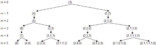
Figure 1: Genealogical tree of self twin games (rows $m$ from 0 to 5 or $n$ from 4 to 9) expressed by their free type representation.

Let us give here rather informally the evolutionary rules that characterize the tree.

Proposition 6.1.

The seed of the genealogical tree (the generation zero game) is the $STP$ “Adamo” four person game, whose free type representation is 3.

Definition 6.1.

A $STP$ game with an odd (respectively an even) number of components in its free type representation ${}_{f}{\bf x}$ is called odd (even) self twin parsimonious, or shortly $OSTP$ ($ESTP$) game.

Proposition 6.2.

All STP games of zero or even generation (m zero or even), are OSTP i.e. they have $h-1$ odd.

Proposition 6.3.

Half of the STP games of any odd generation (m odd) are OSTP (and obviously the other half ESTP).

Definition 6.2.

The central component ${\bf x}_{h/2}$ of the free type representation of an OSTP is called pivot of the representation (or shortly of the game).

Proposition 6.4.

The pivot of an OSTP of any (zero or) even generation is an odd number.

Proposition 6.5.

The pivot of an OSTP of any odd generation is an even number.

Proposition 6.6.

An OSTP $G$ of any even generation, with pivot ${\bf x}_{h/2}$ gives birth to a couple of children STP games of the next (odd) generation, let us denote them by $G^{1}$ and $G^{2}$. $G^{1}$ is OSTP and $G^{2}$ is ESTP.

Proposition 6.7.

The child $G^{1}$ replicates the representation of the parent $G$ except for the pivot which is now (coherently with prop. 6.5) surely an even number ${\bf x}^{1}_{h/2}={\bf x}_{h/2}+1$.

Proposition 6.8.

The child $G^{2}$ is obtained by an almost full replication of the brother $G^{1}$ but (coherently with prop. 6.3) splitting the pivot ${\bf x}_{h/2}+1$ into a couple of equal central components $({\bf x}_{h/2}+1)/2$.

Proposition 6.9.

An OSTP $G^{1}$ of any odd generation, with even pivot ${\bf x}^{1}_{h/2}={\bf x}_{h/2}+1$ gives birth to a unique child OSTP game $G^{11}$ of the next (even) generation. The child replicates the structure of the father (and of the grandfather also) except for the pivot which is now (coherently with prop. 6.5) surely an odd number ${\bf x}^{11}_{h/2}={\bf x}^{1}_{h/2}+1={\bf x}_{h/2}+2$.

Proposition 6.10.

An ESTP $G^{2}$ of any odd generation gives birth to a unique child OSTP game $G^{21}$ of the next (even) generation. The child replicates the structure of the father but with the insertion of the pivot 1 in the previous even representation of $G^{2}$.

Proposition 6.11.

All the games built according to these rules are by construction bilaterally symmetric (hence STP).

Proposition 6.12.

The number of STP (half OSTP, half ESTP) of any odd generation is twice the number of the STP (all OSTP) of the previous generation.

Proposition 6.13.

The number of STP (all OSTP) of any even generation $m$ is the same of the STP of the previous odd generation $m-1$ and twice the number of STP of the previous even $m-2$ generation.

Proposition 6.14.

Prop. 6.1, 6.12 and 6.13 jointly grant that the STP of our genealogical tree exhaust the cardinality of STP games for any value of $n$ (or $m$). Check it through a simple comparison with the values of $\Gamma(m)$ given by Result 4.1.

We may conclude that:

Proposition 6.15.

The genealogical tree introduced in this section fully and unequivocally describes all ST (bilaterally symmetric) Parsimonious games.

In this section we found that the pivot components of $OSTP$ played a key role in the evolutionary rules of the genealogical tree. In the next section we will see that other triangles, no more of the $MPT$ type but nevertheless characterized by significant regularities, are able to describe the evolutionary rule behind the pivot behaviour.

7 The pivot triangles

A pivot triangle is a triangle of numbers whose rows correspond to generations according to their $m$ value; in each row we find the sequences, in increasing order, of all feasible values of the pivots of the $OSTP$ games for the related generation. Columns are labelled by natural numbers $c=1,2,\ldots$. The value of the pivot in row $m$ and column $c$ is $x_{m,c}$, while $r_{m,c}$ is the number of $OSTP$ games of $m$ generation whose pivot is $x_{m,c}$ (shortly repetitions of $x_{m,c}$).

We will distinguish hereafter even triangles, associated to even generations ($m$ zero or even), and odd triangles associated to odd values of $m$.

7.1 The pivot triangles of even generations

Let us consider in this section only the even generations of the tree. For any of the initial even generations, we list here (Table 4) the values $x_{m,c}$ of the pivots involved, as well as (in brackets) the number $r_{m,c}$ of repetitions of each pivot’s value.

$c$
		1	2	3	4	5	6	7
	0	3(1)
	2	1(1)	5(1)
	4	1(2)	3(1)	7(1)
$m$	6	1(4)	3(2)	5(1)	9(1)
	8	1(8)	3(4)	5(2)	7(1)	11(1)
	10	1(16)	3(8)	5(4)	7(2)	9(1)	13(1)
	12	1(32)	3(16)	5(8)	7(4)	9(2)	11(1)	15(1)

Table 4: Even generation pivots triangle

To understand the table note that the evolutionary rules of the genealogical tree imply that going from one even generation, $m$, to the next even, $m+2$, each pivot $x_{m,c}$ gives rise to a couple of grandchildren pivots, whose values are, respectively, $x_{m+2,c+1}=x_{m,c}+2$ and $x_{m+2,1}=1$. Hence, if in the $m$ generation the odd pivot $x_{m,c}$ is repeated $r_{m,c}$ times, the odd pivot $x_{m,c}+2$ is repeated $r_{m,c}=r_{m+2,c+1}$ times in the following $m+2$ generation.

On the other side, Formula (4.1a) implies that the odd pivot $x_{m,1}=1$ is repeated $r_{m+2,1}=2^{m/2}$ times in the $m+2$ generation.

These rules, jointly with the initial condition that in generation 0 there is the unique pivot $x_{0,1}=3$, give a straightforward explanation of the whole table. Let us enter now in some detail.

Proposition 7.1.

For any row $m$ the number of columns, that is of different pivots of $m$ generation, is ${m\over 2}+1$.

Indeed, it is the cardinality of the set of all positive odd integers not greater than $m+3$, except for $m+1$.

The pivots’ values are as follows:

Result 7.1.

$$x_{0,1}=x_{0,(m/2)+1}=3\quad\text{there is just one pivot}$$ (7.1a)

$$x_{m,c}=2c-1\quad\text{for $m$ even and $c=1,\ldots,(m/2)$}$$ (7.1b)

$$x_{m,c}=2c+1\quad\text{for $m$ even and $c=(m/2)+1$}$$ (7.1c)

Put $Z(m)=\sum_{c}x_{m,c}$, the sum of all pivots’ values (without repetitions) of the $m$ generation. Then, it is:

Result 7.2.

$$Z(m)=2+\Big{(}{m\over 2}+1\Big{)}^{2}\text{or}$$ (7.2a)

$$Y(m)=Z(m)-2=\Big{(}{m\over 2}+1\Big{)}^{2}$$ (7.2b)

Proof.

Subtracting 2 to the last entry of each row (the other entries unchanged), we find exactly the well known triangle of squared numbers, i.e. the triangle having on the rows the sequences of all odd integers up to $m+1$, whose sum of entries (on each row) is $\Big{(}{m\over 2}+1\Big{)}^{2}$, that is the sequence of squared natural numbers $(1,4,9,16,\ldots)$. See Table 5. ∎

					$c$
		1	2	3	4	5	6	7	$Y(m)$
	0	1							$1$
	2	1	3						$4$
	4	1	3	5					$9$
$m$	6	1	3	5	7				$16$
	8	1	3	5	7	9			$25$
	10	1	3	5	7	9	11		$36$
	12	1	3	5	7	9	11	13	$49$

Table 5: Squared numbers triangle.

The sum of the row $m+2$ is obtained adding $m+3$ to the sum of the (non bracketed) entries of the previous row $m$ (see Table 4):

Result 7.3.

$$Z(m+2)=Z(m)+(m+3)$$ (7.3)

Proof.

Immediate by Formula (7.2a). An enlightening pivotal explanation is the following: we know that each row (label $m$) has exactly $1+(m/2)$ columns. Going from the $m$ generation to the following, each of the $(m+2)/2$ pivot with value $x$ generates a pivot of value $x+2$; moreover, the pivot 1 is to be added (here we do not care the repetitions). The global increment is then $1+(2\cdot(m+2)/2)=1+(m+2)=m+3$. ∎

As for the repetitions, we have:

Result 7.4.

$$r_{m,c} =2^{(m/2)-c}\quad\text{for $m$ even and $c=1,\ldots,(m/2)$}$$ (7.4a)

$$r_{m,(m/2)+1} =1\quad\text{for $m$ (zero or even) and $c=(m/2)+1$}$$ (7.4b)

This implies:

Result 7.5.

$$r_{m,1} =\sum_{c}r_{m-2,c}$$ (7.5a)

$$r_{m,c} =2\cdot r_{m-1,c}\quad\text{for $m$ even and $c=1,\ldots,(m/2)-1$}$$ (7.5b)

$$r_{m,c} =1\quad\text{for $m$ even and $c=(m/2),(m/2)+1$}$$ (7.5c)

It turns out that the highest rightward diagonal (corresponding to the first row $m=0$) has constant entries equal to 1, while those starting from the other rows ($m$ even), have constant entries $2^{(m/2)-1}$. See Table 6.

$c$
		1	2	3	4	5	6	7
	0	(1)
	2	(1)	(1)
	4	(2)	(1)	(1)
$m$	6	(4)	(2)	(1)	(1)
	8	(8)	(4)	(2)	(1)	(1)
	10	(16)	(8)	(4)	(2)	(1)	(1)
	12	(32)	(16)	(8)	(4)	(2)	(1)	(1)

Table 6: Pivot repetitions triangle

Finally, as for the sum $\Phi(m)$ of all pivots value on each row (keeping account of the repetitions), it is for any $m$ (zero or even):

Result 7.6.

$$\Phi(m)=\sum_{c}x_{m,c}\cdot r_{m,c}=2^{m/2}\cdot 3$$ (7.6)

Proof.

Immediate by induction. It is true for $m=0$; let us check that if it is true for any even $m$, it is true for the next even $(m+2)$. It is:

$$\begin{split}\Phi(m+2)&=\sum_{c}x_{m+2,c}\cdot r_{m+2,c}=\sum_{c}(x_{m,c}+3)\cdot r_{m,c}=\\ &=\sum_{c}x_{m,c}\cdot r_{m,c}+3\cdot\sum_{c}r_{m,c}=\Phi(m)+3\cdot 2^{m/2}=\\ &=2^{m/2}\cdot 3+3\cdot 2^{m/2}=2\cdot 2^{m/2}\cdot 3=2^{(m+2)/2}\cdot 3\\ \end{split}$$ (7.7)

∎

7.2 The pivot triangles of odd generations

Let us consider now the behaviour of the odd generations ($m=1,3,\ldots$) and in particular the pivot elements of the subset with odd representation. It turns out that it mimics (mutatis mutandis) the rule driving the even generation one; this fact may be perceived by the following table:

$c$
		1	2	3	4	5
	1	4(1)
	3	2(1)	6(1)
$m$	5	2(2)	4(1)	8(1)
	7	2(4)	4(2)	6(1)	10(1)
	9	2(8)	4(4)	6(2)	8(1)	12(1)

Table 7: Odd generation pivot triangle

To understand the behaviour of the new triangle requires nothing but to adapt all properties.

Let $x^{{}^{\prime}}_{m^{{}^{\prime}},c}$ and $r^{{}^{\prime}}_{m^{{}^{\prime}},c}$ be the entries of the odd triangle, with $m^{{}^{\prime}}=m+1$ ($m$ even). It is immediate to check that, for any $m^{{}^{\prime}},c$, we have:

Proposition 7.2.

$$x^{{}^{\prime}}_{m^{{}^{\prime}},c}=x_{m,c}+1$$ (7.8)

$$r^{{}^{\prime}}_{m^{{}^{\prime}},c}=r_{m,c}$$ (7.9)

Exploiting Formulas (7.8) and (7.9) it is easy to obtain the counterpart of all results given in the previous subsection. Here, we provide only the analogous of Formula (7.6). Putting

$$\Psi(m^{{}^{\prime}})=\sum_{c}x^{{}^{\prime}}_{m^{{}^{\prime}},c}\cdot r_{m^{{}^{\prime}},c}$$

it is:

Result 7.7.

$$\Psi(m^{{}^{\prime}})=2^{(m^{{}^{\prime}}-1)/2}\cdot 4$$ (7.10)

Proof.

It is:

$$\begin{split}\Psi(m^{{}^{\prime}})&=\sum_{c}x^{{}^{\prime}}_{m^{{}^{\prime}},c}\cdot r_{m^{{}^{\prime}},c}=\sum_{c}(x_{m,c}+1)\cdot r_{m,c}=\\ &=\sum_{c}x_{m,c}\cdot r_{m,c}+\sum_{c}r_{m,c}=\Phi(m)+2^{m/2}=\\ &=2^{m/2}\cdot 3+2^{m/2}=4\cdot 2^{m/2}=4\cdot 2^{(m^{{}^{\prime}}-1)/2}\\ \end{split}$$ (7.11)

∎

8 Examples

Example 8.1.

The first example keeps $m=4$, that is $n=8$. There are $2^{4}=16$ $P$ games, 4 of which are self twin, while the other 12 may be seen as 6 pairs of non identical twins. Table 3 reveals that those pairs may be divided in 3 groups with respectively three, four or five types. Each group contains 2 pairs of non identical twins. Here the complete list of the 16 $P$ games, grouped by their $h$ value and expressed through their free type representation (in parenthesis) with $h-1$ components.

$h=2$:	(7)	self twin
$h=3$:	(3,4) and (4,3)	first pair of twins
	(2,5) and (5,2)	second pair of twins
$h=4$:	(2,3,2)	first self twin
	(3,1,3)	second self twin
	(2,1,4) and (4,1,2)	first pair of twins
	(2,2,3) and (3,2,2)	second pair of twins
$h=5$:	(2,1,2,2) and (2,2,1,2)	first pair of twins
	(2,1,1,3) and (3,1,1,2)	second pair of twins
$h=6$:	(2,1,1,1,2)	self twin

The corresponding rows of our $MPT$ are ($m=4$, $k$ from 0 to 4):

$$C:1,4,6,4,1$$

$$\Gamma:1,0,2,0,1$$

$$\Delta:0,4,4,4,0$$

$$\Theta:0,2,2,2,0$$

The minimal homogeneous representations are:

$h=2$:	(7;1,1,1,1,1,1,1,6)
$h=3$:	(13;1,1,1,3,3,3,3,10)	(13;1,1,1,1,4,4,4,9)
	(11;1,1,2,2,2,2,2,9)	(11;1,1,1,1,1,5,5,6)
$h=4$:	(16;1,1,2,2,2,7,7,9)
	(15;1,1,1,3,4,4,4,11)
	(14;1,1,2,3,3,3,3,11)	(14;1,1,1,1,4,5,5,9)
	(17;1,1,2,2,5,5,5,12)	(17;1,1,1,3,3,7,7,10)
$h=5$:	(19;1,1,2,3,3,8,8,11)	(19;1,1,2,2,5,7,7,12)
	(18;1,1,2,3,5,5,5,13)	(18;1,1,1,3,4,7,7,11)
$h=6$:	(21;1,1,2,3,5,8,8,13)

It is interesting to observe that (as proved in [13],Theorem T5.1, sect. 5.1), all pairs of twins have the same minimal winning quota $q$ (of course pair dependent).

Example 8.2

The second example keeps $n=9$ ($m=5$). There are 32 $P$ games, 8 of which self twin, while the other 24 may be divided in 12 pairs of twins.

Here the complete list of the 32 $P$ games, grouped by their $h$ value:

$h=2$:	(8)	self twin
$h=3$:	(4,4)	self twin
	(3,5) and (5,3)	first pair of twins
	(2,6) and (6,2)	second pair of twins
$h=4$:	(2,4,2)	first self twin
	(3,2,3)	second self twin
	(2,1,5) and (5,1,2)	first pair of twins
	(2,2,4) and (4,2,2)	second pair of twins
	(2,3,3) and (3,3,2)	third pair of twins
	(3,1,4) and (4,1,3)	forth pair of twins
$h=5$:	(2,2,2,2)	first self twin
	(3,1,1,3)	second self twin
	(2,1,1,4) and (4,1,1,2)	first pair of twins
	(2,1,2,3) and (3,2,1,2)	second pair of twins
	(2,1,3,2) and (2,3,1,2)	third pair of twins
	(3,1,2,2) and (2,2,1,3)	forth pair of twins
$h=6$:	(2,1,2,1,2)	self twin
	(2,1,1,2,2) and (2,2,1,1,2)	first pair of twins
	(2,1,1,1,3) and (3,1,1,1,2)	second pair of twins
$h=7$:	(2,1,1,1,1,2)	self twin

The corresponding rows of our $MPT$ are ($m=5$, $k$ from 0 to 5):

$$C:1,5,10,10,5,1$$

$$\Gamma:1,1,2,2,1,1$$

$$\Delta:0,4,8,8,4,0$$

$$\Theta:0,2,4,4,2,0$$

The minimal homogeneous representations are:

$h=2$:	(8;1,1,1,1,1,1,1,1,7)
$h=3$:	(17;1,1,1,1,4,4,4,4,13)
	(16;1,1,1,3,3,3,3,3,13)	(16;1,1,1,1,1,5,5,5,11)
	(13;1,1,2,2,2,2,2,2,11)	(13;1,1,1,1,1,1,6,6,7)
$h=4$:	(20;1,1,2,2,2,2,9,9,11)
	(24;1,1,1,3,3,7,7,7,17)
	(17;1,1,2,3,3,3,3,3,14)	(17;1,1,1,1,1,5,6,6,11)
	(22;1,1,2,2,5,5,5,5,17)	(22;1,1,1,1,4,4,9,9,13)
	(23;1,1,2,2,2,7,7,7,16)	(23;1,1,1,3,3,3,10,10,13)
	(19;1,1,1,3,4,4,4,4,15)	(19;1,1,1,1,4,5,5,5,14)
$h=5$:	(29;1,1,2,2,5,5,12,12,17)
	(25;1,1,1,3,4,7,7,7,18)
	(23;1,1,2,3,5,5,5,5,18)	(23;1,1,1,1,4,5,9,9,14)
	(27,1,1,2,3,3,8,8,8,19)	(27;11,1,1,3,3,7,10,10,17)
	(25;1,1,2,3,3,3,11,11,14)	(25;1,1,2,2,2,7,9,9,16)
	(26;1,1,1,3,4,4,11,11,15)	(26;1,1,2,2,5,7,7,7,19)
$h=6$:	(30;1,1,2,3,3,8,11,11,19)
	(31;1,1,2,3,5,5,13,13,18)	(31;1,1,2,2,5,7,12,12,19)
	(29;1,1,2,3,5,8,8,8,21)	(29;1,1,1,3,4,7,11,11,18)
$h=7$:	(34;1,1,2,3,5,8,13,13,21)

9 Conclusions

In this paper we discuss the role of modified Pascal triangles in describing the cardinality of self twin (bilaterally symmetric) Parsimonious games for any combination of the relevant parameters $m,k$ associated respectively to the number $n=m+4$ of players and $h=k+2$ of types in the game. In detail, we show that the entries of the modified triangles follow almost wholly (with a slight modification) the evolutionary rule embedded in the basic combinatorial relation (Pascal equation) which gives any binomial coefficient as the sum of two adjacent coefficient of the previous row of the classic Pascal triangle. In addition we also provide a genealogical tree of self twin games, in which each game of a given generation (corresponding to a value of $m$) is able to give birth to one or two (depending on the parity of $m$) children self twin games of the next generation. The breeding rules, defined in terms of the free type representation, are, given the parity, invariant across generations. They are quite simple and may be translated in an high speed pen and pencil constructive procedure to obtain all self twin games for small enough values of $n$; obviously a simple computational routine produces the set of all self twin games also for large values of $n$ with the only constraint of the computational power (recall that the number of self twin games explodes at the rhythm of the square root of $2^{n-4}$).

The analysis of the genealogical tree revealed that a key role in its evolution is played by the pivot components of the subset of self twin Parsimonious games whose free type representation has an odd number of components. We found that other triangles (pivot triangles) describe the structure of the pivot’s set and give a synthesis of their evolutionary pattern.

We are aware that our paper is wholly theoretical so we leave to subsequent research to look for practical applications to hard or social sciences. Indeed, we hope that such results could follow given the prominent role played by bilateral symmetry in many fields of the life of the universe.

Appendix A Appendix: proof of the proposition 3.1

Define ${\bf I}({\bf b})=(I_{1},I_{2},\ldots,I_{h})$ as the vector of ordinal labellings of 1’s of ${\bf b}$.

For example, if ${\bf b}=(1,0,1,0,1,1,0,1,0,1)$, ${\bf I}({\bf b})=(1,3,5,6,8,10)$.

It follows that, for $t=1,\ldots,h-1$, it is:

$$x_{t}=I_{t+1}-I_{t}\quad\text{and }\quad x_{h}=1$$

Conversely, for any $t>2$, it is:

$$I_{t}=1+\sum_{j=1}^{t-1}x_{j}\quad\text{and }\quad I_{1}=1$$

In the example: $x_{1}=3-1=2$, $x_{2}=5-3=2$, $x_{3}=6-5=1$, $x_{4}=8-6=2$, $x_{5}=10-8=2$ and $x_{6}=1$, or ${}_{f}{\bf x}=(2,2,1,2,2)$.

Hypothesis: ${}_{f}{\bf b}$ bilaterally symmetric, hence ${\bf b}$ bilaterally symmetric. See Proposition 3.1.

We show that this implies that also ${}_{f}{\bf x}$ is bilaterally symmetric.

Proposition A.1.

Bilateral symmetry of ${\bf b}$ is equivalent to the following property of ${\bf I}({\bf b})$:

Property A.1.

For any couple of symmetric subscripts $t$ and $h+1-t$ (sum of subscripts $h+1$) it is:

$$I_{t}+I_{h+1-t}=n+1$$

In the example, it is:

$$I_{1}+I_{6}=1+10=I_{2}+I_{5}=3+8=I_{3}+I_{4}=5+6=10+1$$

Considering now the difference $(x_{t}-x_{h-t})$, it is for any $t=1,\ldots,h-1$:

$$x_{t}-x_{h-t}=(I_{t+1}-I_{t})-(I_{h+1-t}-I_{h-t})=(I_{t+1}+I_{h-t})-(I_{t}+I_{h+1-t})=(n+1)-(n+1)=0$$

The last but one equality is a consequence of Property A.1, keeping account that the sum of indices of the terms in both brackets is $h+1$. Hence $x_{t}-x_{h-t}=0$, which means that ${}_{f}{\bf x}$ is bilaterally symmetric.

Conversely, hypothesis: ${}_{f}{\bf x}$ bilaterally symmetric. We show that this implies that also ${}_{f}{\bf b}$ is bilaterally symmetric.

By hypothesis, for any $t=1,\ldots,h-1$, it is:

$$x_{t}=x_{h-t}$$

Substitution gives:

$$I_{t+1}-I_{t}=I_{h+1-t}-I_{h-t}$$

equivalent to:

$$I_{t+1}+I_{h-t}=I_{t}+I_{h+1-t}$$

The sum of subscripts in both sides of the equation is $h+1$, thus Property A.1 is satisfied and, by proposition A.1 this implies bilateral symmetry of ${\bf b}$.

Appendix B Appendix: proofs of evolutionary rules of the $MPT$ $\Gamma$

Proof.

Case $m$ even, $k$ even. Recalling Formula (4.2a), it is:

$$\Gamma(m,k)=C(m/2,k/2)$$ (B.1)

Now, denoting by $m^{{}^{\prime}}=m-1$ and $k^{{}^{\prime}}=k-1$ both odd and keeping account of Formula (4.2c):

$$\Gamma(m-1,k)=\Gamma(m^{{}^{\prime}},k)=C\Big{(}(m^{{}^{\prime}}-1)/2,k/2\Big{)}=C\Big{(}(m/2)-1,k/2\Big{)}$$ (B.2)

while, applying Formula (4.2d):

$$\Gamma(m-1,k-1)=\Gamma(m^{{}^{\prime}},k^{{}^{\prime}})=C\Big{(}(m^{{}^{\prime}}-1)/2,(k^{{}^{\prime}}-1)/2\Big{)}=C\Big{(}(m/2)-1,(k/2)-1\Big{)}$$ (B.3)

Being

$$C\Big{(}m/2,k/2\Big{)}=C\Big{(}(m/2)-1,(k/2)\Big{)}+C\Big{(}(m/2)-1,(k/2)-1\Big{)}$$

we found that Formula (5.2) is satisfied. ∎

Proof.

Case $m$ odd, $k$ odd. Recalling Formula (4.2d), it is:

$$\Gamma(m,k)=C\Big{(}(m-1)/2,(k-1)/2\Big{)}$$ (B.4)

In turn, for Formula (4.2b):

$$\Gamma(m-1,k)=0$$ (B.5)

while, applying Formula (4.2a):

$$\Gamma(m-1,k-1)=\Gamma(m^{{}^{\prime}},k^{{}^{\prime}})=C\Big{(}m^{{}^{\prime}}/2,k^{{}^{\prime}}/2\Big{)}=C\Big{(}(m-1)/2,(k-1)/2\Big{)}$$ (B.6)

so that we found again that Formula (5.2) is satisfied. ∎

Proof.

Case $m$ odd, $k$ even. Recalling Formula (4.2c), it is:

$$\Gamma(m,k)=C\Big{(}(m-1)/2,k/2\Big{)}$$ (B.7)

Now, keeping account of Formula (4.2a):

$$\Gamma(m-1,k)=\Gamma(m^{{}^{\prime}},k)=C\Big{(}m^{{}^{\prime}}/2,k/2\Big{)}=C\Big{(}(m-1)/2,k/2\Big{)}$$ (B.8)

on the other side, applying Formula (4.2b) ($m-1$ even, $k-1$ odd):

$$\Gamma(m-1,k-1)=0$$ (B.9)

So that Formula (5.3) is satisfied. ∎

Proof.

Case $m$ even, $k$ odd. Recalling Formula (4.2b), it is:

$$\Gamma(m,k)=0$$ (B.10)

and let us check that:

$$\Gamma(m-1,k)=\Gamma(m-1,k-1)$$ (B.11)

Indeed

$$\Gamma(m-1,k)=\Gamma(m^{{}^{\prime}},k)=C\Big{(}(m^{{}^{\prime}}-1)/2,(k-1)/2\Big{)}$$ (B.12)

while

$$\Gamma(m-1,k-1)=\Gamma(m^{{}^{\prime}},k^{{}^{\prime}})=C\Big{(}(m^{{}^{\prime}}-1)/2,k^{{}^{\prime}}/2\Big{)}=C\Big{(}(m^{{}^{\prime}}-1)/2,(k-1)/2\Big{)}$$ (B.13)

Again Formula (5.3) is satisfied. ∎

References

- [1] Ando S., (1988), A Triangular Array with Hexagon Property, Dual to Pascal’s Triangle, Application of Fibonacci numbers, Springer Netherlands, 61-67
- [2] Barry P., (2006), On integer sequence based constructions of generalized Pascal triangles, Journal of Integer Sequences, 9, 1-34
- [3] Bollinger R. C., (1993), Extended Pascal triangles, Mathematics Magazine, 66, no. 2, 87-94
- [4] Brading K. and E. Castellani, (2003), Symmetries in physics: philosophical reflections, Cambridge University Press
- [5] Finnerty J. R., (2003), The Origins of axial patterning in metazoa: how old is bilateral symmetry, International Journal Development Biology, 47, (7-8), 523-529
- [6] Gardner D., (1971), Bilateral Symmetry and Interneuronal Organization in the Buccal Ganglia of Aplysia, Science, 173, no. 3996 550-553
- [7] Granville A., (1992), Zaphod Beeblebrox’s Brian and the Fifty-ninth Row of Pascal’s Triangle Andrew Granville, The American Mathematical Monthly, 99, no. 4, 318-331
- [8] Horowitz A.D., (1973), The Competitive Bargaining Set for Cooperative n-Person Games, Journal of Mathematical Psychology 10, 265-289
- [9] Isbell R., (1956), A class of majority games, Quarterly Journal of Mathematics, 7, 183-187
- [10] Møller A. P. and R. Thornhill, (1998), Bilateral Symmetry and Sexual Selection: A Meta-Analysis, The American Naturalist, 151, no. 2, 174-192
- [11] Ostmann A., (1987), On the minimal representation of homogeneous games, International Journal of Game Theory, 16, 69-81
- [12] Palmer A. R., (2004), Symmetry Breaking and the Evolution of Development, Science, 306, no. 5697, 828-833
- [13] Pressacco F. and G. Plazzotta, (2013), Symmetry and twin relationships in Parsimoniuos games, CEPET Working paper, 2013-2
- [14] Rosen J., (1996), Symmetry in Science: an introduction to the general theory, Springer
- [15] Rosenmüller J., (1987), Homogeneous games: recursive structure and Mathematics of Operations Research, 12-2, 309-330
- [16] Song H. et al, (2010), Planar cell polarity breaks bilateral symmetry by controlling ciliary positioning, Nature, 466, 368-372
- [17] Trzaska W., (1991), Modified numerical triangle and the Fibonacci sequence, Fibonacci Quarterly
- [18] Von Neumann J. and O. Morgenstern, (1947), Theory of games and economic behaviour, Princeton University Press
- [19] Weyl H., (1952), Symmetry, Princeton University Press
- [20] Wiener E., (2012), The origin evolution and development of bilateral symmetry in multicellular organism, Tissues and Organs, ArXiv:1207.3289 (q.bio.TO)