A Mixed ODE-PDE Model for Vehicular Traffic

Abstract

We present a traffic flow model consisting of a gluing between the Lighthill–Whitham and Richards macroscopic model with a first order microscopic follow the leader model. The basic analytical properties of this model are investigated. Existence and uniqueness are proved, as well as the basic estimates on the dependence of solutions from the initial data. Moreover, numerical integrations show some qualitative features of the model, in particular the transfer of information among regions where the different models are used.

2000 Mathematics Subject Classification: 35L65, 90B20

Key words and phrases: Continuum Traffic Models, Hyperbolic Systems of Conservation Laws, Microscopic Traffic Models

1 Introduction

We consider a traffic flow model consisting of a macroscopic and a microscopic descriptions glued together. The macroscopic part is described through the Lighthill–Whitam [13] and Richards [14] model (LWR)

$$\partial_{t}\rho+\partial_{x}\left(\rho\,v(\rho)\right)=0,$$ (1.1)

which is a scalar conservation law, where the unknown $\rho=\rho(t,x)$ is the (mean) traffic density and $v=v(\rho)$ is the (mean) traffic speed. Microscopic models for vehicular traffic consist of a finite set of ordinary differential equations, describing the motion of each vehicle in the traffic flow. Below, as in [2], we consider a first order Follow–the–Leader (FtL) model, where each driver adjusts his/her velocity to the vehicle in front, that is

$$\dot{p}_{i}=v\left(\frac{\ell}{p_{i+1}-p_{i}}\right).$$ (1.2)

Here, $p_{i}=p_{i}(t)$ is the position of the $i$-th driver, for $i=1,\ldots,n$, and $p_{i+1}-p_{i}\geq\ell$ for all $i=1,\ldots,n-1$, the fixed parameter $\ell$ denoting the (mean) vehicles’ length. Here, $\ell/(p_{i+1}-p_{i})$ is the local traffic density in front of the driver $p_{i}$. Equation (1.2) needs to be closed with the trajectory of the first driver $p_{n}$.

In general, the two descriptions (1.1) and (1.2) can be alternatively used in different segments of the real line. The resulting model, in general, consists of several instances of (1.1) and (1.2) alternated along the real line, separated by free boundaries, whose evolution needs to be determined. This description enjoys the basic properties in [9] that are there considered as necessary for a reliable description of traffic dynamics. Indeed, density and speed are a priori bounded, speed is never negative and vanishes only at the maximal density.

A similar approach to traffic modeling is in [10], where the interface between the micro- and macro description is kept fixed and the model in [3, 15] plays the role here played by the LWR one. See also [7] for the case $n=1$.

From a macroscopic point of view, vehicular traffic can be viewed as a compressible fluid flow, whereas a microscopic approach describes the behavior of each individual vehicle. Macroscopic descriptions allow to simulate traffic on large networks but do not take much account of the details. On the other hand, microscopic descriptions can cover such details, but they are not tractable on a large network. None of the two approaches is separately able to capture the information of traffic dynamics. A natural strategy is therefore to combine macroscopic and microscopic models. The result is the present Micro–Macro Model, consisting in the coupling of the two different descriptions.

Numerical results complete the study of the model and show the reasonableness of it’s solutions: in particular they explain how the two micro- and macroscopic descriptions coexist in a single model, although being separated. Below, we prove a well posedness result separately for the LWR-FtL case, when the LWR model describes the traffic dynamics on the right and the FtL on the left, and for the opposite case, the FtL-LWR one; we also provide precise estimates on how the solution depends from the initial data.

The paper is organized as follows: in the next section we introduce the notations and the general model, when the two descriptions are alternatively used in different segments of the real line. Then, we prove a well posedness result separately for the LWR-FtL case and the FtL-LWR one. In Section 3 we present some numerical results related to the model. All proofs are gathered in the last section.

2 Notation and Main Results

Throughout, we denote ${\mathbb{R}}^{+}=\left[0,+\infty\right[$ and $\mathaccent 23{{\mathbb{R}}}^{+}=\left]0,+\infty\right[$. For any $n\in{\mathbb{N}}$ and $\ell\in\mathaccent 23{{\mathbb{R}}}^{+}$, the set of admissible positions of $n$ vehicles of length $\ell$ is

$$\mathcal{P}_{\ell}^{n}=\left\{p\in{\mathbb{R}}^{n}\colon p_{i+1}-p_{i}\geq\ell\mbox{ for }i=1,\ldots,n-1\right\}\,.$$ (2.1)

Throughout, we assume the following condition on the speed law:

(v)

$v\in\mathbf{C^{2}}([0,1];{\mathbb{R}}^{+})$ is strictly decreasing, with $v(1)=0$ and is such that $\frac{d^{2}~{}}{d\rho^{2}}\left(\rho\,v(\rho)\right)<0$.

Our aim is the well posedness of a system consisting of various instances of the LWR model (1.1) and of the FtL model (1.2), alternated along the real line. To this aim, introduce the number $N\in{\mathbb{N}}$, $N\geq 1$, of the intervals where the FtL model is used. Call $n_{j}$, with $n_{j}\geq 2$ for $j=1,\ldots,N$, the number of individuals in the $j$-th interval and denote $\mathcal{I}_{p}(t)$ the set of those points in ${\mathbb{R}}$ where the macroscopic model is used, i.e.

$$\mathcal{I}_{p(t)}=\left]-\infty,p_{1}^{1}(t)\right[\cup\bigcup_{j=1}^{N-1}\left]p_{n_{j}}^{j}(t),p_{1}^{j+1}(t)\right[\cup\left]p_{n_{N}}^{N}(t),+\infty\right[\,,$$

see Figure 1. Consider the system

$$\!\!\!\left\{\begin{array}[]{@{}l@{\qquad}l@{}}\partial_{t}\rho+\partial_{x}\left(\rho\,v(\rho)\right)=0&\displaystyle x\in\mathcal{I}_{p(t)}\\ \dot{p}_{i}^{j}(t)=v\left(\frac{\ell}{p_{i+1}^{j}(t)-p_{i}^{j}(t)}\right)&i=1,\ldots,n_{j}-1\,,\qquad j=1,\ldots,N\\ \dot{p}_{n_{j}}^{j}=v\left(\rho\left(t,p_{n_{j}}^{j}(t)\right)\right)&j=1,\ldots,N\\ \rho(0,x)=\bar{\rho}(x)&\displaystyle x\in\mathcal{I}_{\bar{p}}\\ p^{j}(0)=\bar{p}^{j}&j=1,\ldots,N\,,\end{array}\right.$$ (2.2)

Throughout, we require that the initial data satisfy the admissibility condition

$$\begin{array}[]{rcll}\bar{\rho}&\in&(\mathbf{L^{1}}\cap\mathbf{BV})({\mathbb{R}};[0,1])&\mbox{ with }\bar{\rho}(x)=x\mbox{ whenever }x\in{\mathbb{R}}\setminus\mathcal{I}_{\bar{p}}\,,\\ \bar{p}^{j}&\in&\mathcal{P}_{\ell}^{n_{j}}&\mbox{ for all }\quad j=1,\ldots,N\,.\end{array}$$ (2.3)

\psfrag{r}{$\rho$}\psfrag{x}{$x$}\psfrag{t}{$t$}\psfrag{p11}{$p_{1}^{1}$}\psfrag{p12}{$p_{n_{1}}^{1}$}\psfrag{p21}{$p_{1}^{2}$}\psfrag{p22}{$p_{n_{2}}^{2}$}\includegraphics[width=303.53267pt]{situation.eps}

Figure 1: Situation described by (2.2) in the case $N=2$, $n_{1}=5$ and $n_{2}=3$.

Note that problems similar to (2.2) can be stated equally with the microscopic model in the rightmost and/or leftmost part of the real line.

The first step in the rigorous treatment of (2.2) is the definition of its solutions. Essentially, we require to solve the ordinary differential equations in (2.2) as usual and to seek a weak entropy (Kružkov) solution to the hyperbolic conservation law (1.1) in $\mathcal{I}_{p}(t)$, for $t\in{\mathbb{R}}^{+}$. To simplify the notation, we require $\rho(t,\cdot)$ to be defined on all the real line and extend it to $0$ on ${\mathbb{R}}\setminus\mathcal{I}_{p}(t)$.

Definition 2.1.

Fix positive $T$ and $\ell$, an initial distribution $\bar{\rho}\in(\mathbf{L^{1}}\cap\mathbf{BV})({\mathbb{R}};[0,1])$ and positions $\bar{p}_{i}^{j}$ for $i=1,\ldots,n_{j}$, $j=1,\ldots,N$ satisfying (2.3). A solution to (2.2) on the time interval $[0,T[$, consists of maps

$$\rho \in \mathbf{C^{0}}\left([0,T];(\mathbf{L^{1}}\cap\mathbf{BV})({\mathbb{R}};[0,1])\right)\quad\mbox{ with }\rho(t,x)=0\mbox{ whenever }x\in{\mathbb{R}}\setminus\mathcal{I}_{p}(t)$$

$$p^{j} \in \mathbf{W^{1,\infty}}([0,T];\mathcal{P}_{\ell}^{n_{j}})\quad\mbox{ for }j=1,\ldots,N$$

(where continuity is understood with respect to the $\mathbf{L^{1}}$ topology) such that

1. for all $\varphi\in\mathbf{C_{c}^{1}}(\left]0,T\right[\times{\mathbb{R}},{\mathbb{R}}^{+})$ with $\mathop{\mathrm{spt}}\varphi\subset\left\{(t,x)\in[0,T]\times{\mathbb{R}}\colon\displaystyle x\in\mathcal{I}_{p}(t)\right\}$ the following inequality holds for all $k\in{\mathbb{R}}$:

   $$\int_{0}^{T}\int_{{\mathbb{R}}}\left({\left|\rho(t,x)-k\right|}\,\partial_{t}\varphi(t,x)+\left(\rho(t,x)\,v\left(\rho(t,x)-k\,v(k)\right)\right)\partial_{x}\varphi(t,x)\right)\mathinner{\mathrm{d}{x}}\,\mathinner{\mathrm{d}{t}}\geq 0\,.$$

2. For $j=1,\ldots,N$ and for a.e. $\tau\in{\mathbb{R}}^{+}$, let $u^{\tau}$ be the solution to the Riemann Problem

   $$\left\{\begin{array}[]{l}\partial_{t}u+\partial_{x}\left(u\,v(u)\right)=0\\ u(t,x)=\left\{\begin{array}[]{l@{\quad\mbox{if }}rcl}\rho(\tau,p_{1}^{j}(\tau)-)&x&<&p_{1}^{j}(\tau)\,,\\ \frac{\ell}{p_{2}^{j}(\tau)-p_{1}^{j}(\tau)}&x&>&p_{1}^{j}(\tau)\,.\end{array}\right.\end{array}\right.$$

   Then, $\rho(t,p_{1}^{j}(t)-)=u^{\tau}(t,x)$, for all $(t,x)$ such that $x<p_{1}^{j}(\tau)+\dot{p}_{1}^{j}(\tau)(t-\tau)$ and $t>\tau$;

3. for a.e. $t\in[0,T]$ and all $j=1,\ldots,N$, $i=1,\ldots,n_{j}-1$, $\dot{p}_{j}^{i}(t)=v\left(l\middle/\left(p_{j}^{i+1}(t)-p_{j}^{i}(t)\right)\right)$;

4. for a.e. $t\in[0,T]$ and all $j=1,\ldots,N$, $\dot{p}_{n_{j}}^{j}(t)=v\left(\rho\left(t,p_{n_{j}}^{j}(t)+\right)\right)$.

Above, the condition at 1. is equivalent to the usual definition of Kružkov solution, see [4, Formula (6.3)]. Thanks to the $\mathbf{L^{1}}$ continuity in times, it also ensures the usual distributional condition: for all $\varphi\in\mathbf{C_{c}^{1}}(\left]-\infty,T\right]\times{\mathbb{R}},{\mathbb{R}})$ with $\mathop{\mathrm{spt}}\varphi\subset\left\{(t,x)\in{\mathbb{R}}^{2}\colon x\in\mathcal{I}_{p}(t)\mbox{ for all }t\in[0,T]\right\}$,

$$\int_{0}^{T}\int_{{\mathbb{R}}}\left(\rho(t,x)\,\partial_{t}\varphi(t,x)+\rho(t,x)\,v\left(\rho(t,x)\right)\,\partial_{x}\varphi(t,x)\right)\mathinner{\mathrm{d}{x}}\mathinner{\mathrm{d}{t}}+\int_{\mathbb{R}}\bar{\rho}(x)\,\varphi(0,x)\mathinner{\mathrm{d}{x}}=0\,.$$

The requirement 2. is the standard definition of solution to a boundary value problem for a conservation law, see [8, Definition 2.1], [1, Definition C.1] and [5, Definition 2.2]. Remark that the trajectories $p_{1}^{j}=p_{1}^{j}(t)$ and $p_{n_{j}}^{j}=p_{n_{j}}^{j}(t)$, for $j=1,\ldots,N$, are free boundaries between micro- and macroscopic descriptions, to be found while solving (2.2). However, only the $p_{1}^{i}$, for $i=1,\ldots,N$, have a role in 2.

We remark that any solution to (2.2) in the sense of Definition 2.1 enjoys the basic properties underlined in [9], namely:

P1

Cars may have only positive speed.

P2

Vehicles stop only at maximum density, i.e., the velocity $v$ is $0$ if and only if the density $\rho$ is equal to the maximum density possible.

The next two sections deal with the two possible gluing of the a single instance of the LWR model and a single instance of the FtL one.

2.1 The Case LWR–FtL

Let $n$ vehicles start at time $t=0$ from positions $\bar{p}\in\mathcal{P}_{\ell}^{n}$ and use the LWR model to describe the traffic dynamics for $x<\bar{p}_{1}$. We are thus lead to consider the problem

$$\left\{\begin{array}[]{@{}l@{\quad}rcll@{}}\partial_{t}\rho+\partial_{x}\left(\rho\,v(\rho)\right)=0&t&\in&{\mathbb{R}}^{+}&\mbox{ and }x\,<\,p_{1}(t)\\ \dot{p}_{i}=v\left(\frac{\ell}{p_{i+1}-p_{i}}\right)&t&\in&{\mathbb{R}}^{+}&\mbox{ and }i=1,\ldots,n-1\\ \dot{p}_{n}=w(t)&t&\in&{\mathbb{R}}^{+}\\ \rho(0,x)=\bar{\rho}(x)&x&\leq&\bar{p}_{1}\\ p(0)=\bar{p}\end{array}\right.$$ (2.4)

where $w\in\mathbf{L^{\infty}}({\mathbb{R}}^{+};{\mathbb{R}}^{+})$ is the speed of the leader, $\bar{\rho}\in(\mathbf{L^{1}}\cap\mathbf{BV})({\mathbb{R}};[0,1])$ describes the vehicles’ distribution for $x<\bar{p}_{1}$ and $\bar{p}\in\mathcal{P}_{\ell}^{n}$. In the present case (2.4), the trajectory of $p_{1}$, i.e., $p_{1}(t)+\bar{p}_{1}+\int_{0}^{t}w(\tau)\mathinner{\mathrm{d}{\tau}}$, acts as a boundary between the microscopic model on its right and the macroscopic one on its left.

Remark that from a strictly rigorous point of view, problem (2.4) does not fit into (2.2). However, the extension of Definition 2.1 to the case of (2.4) is straightforward and we omit it.

Proposition 2.2.

Fix $\ell>0$, $V>0$, $n\in{\mathbb{N}}$ with $n\geq 2$ and a $v$ that satisfies (v). Let $w$ be in $\mathbf{L^{\infty}}({\mathbb{R}}^{+};[0,V])$. For any $\bar{p}\in\mathcal{P}^{n}_{\ell}$ and for any $\bar{\rho}\in(\mathbf{L^{1}}\cap\mathbf{BV})({\mathbb{R}};[0,1])$, problem (2.4) admits a unique solution in the sense of Definition 2.1. Moreover, there exists a positive $L$ such that if $w^{\prime}\in\mathbf{L^{\infty}}({\mathbb{R}}^{+};[0,V])$, $\bar{p}^{\prime}\in\mathcal{P}^{n}_{\ell}$ and $\bar{\rho}^{\prime}\in(\mathbf{L^{1}}\cap\mathbf{BV})({\mathbb{R}};[0,1])$, then the corresponding solutions $(p,\rho)$ and $(p^{\prime},\rho^{\prime})$ satisfy for all $t\geq 0$ the following estimates:

$${\left\|\rho(t,\cdot)-\rho^{\prime}(t,\cdot)\right\|}_{\mathbf{L^{1}}} \leq L{\left\|\bar{\rho}-\bar{\rho}^{\prime}\right\|}_{\mathbf{L^{1}}}$$

$$+ L\left(1+\left(1+2V\right)\frac{2}{\ell}t\right)\left({\left\|\bar{p}-\bar{p}^{\prime}\right\|}+{\left\|w-w^{\prime}\right\|}_{\mathbf{L^{1}}([0,t])}\right)\exp\left(2\frac{\mathbf{Lip}(v)}{\ell}t\right)$$

$${\left\|p(t)-p^{\prime}(t)\right\|} \leq \left({\left\|\bar{p}-\bar{p}^{\prime}\right\|}+{\left\|w-w^{\prime}\right\|}_{\mathbf{L^{1}}([0,t])}\right)\exp\left(2\,\frac{\mathbf{Lip}(v)}{\ell}\,t\right)\,.$$

The proof is postponed to Section (4).

2.2 The Case FtL–LWR

Next we use the FtL model to describe $n$ vehicles starting at time $t=0$ from positions $\bar{p}\in\mathcal{P}_{\ell}^{n}$ and the LWR model for $x>p_{n}(t)$. The free boundary between the two models is the trajectory $p_{n}=p_{n}(t)$, chosen so that $\dot{p}_{n}=v\left(\rho(t,p_{n}(t))\right)$. We are thus lead to consider the problem

$$\left\{\begin{array}[]{@{}l@{\quad}rcll@{}}\partial_{t}\rho+\partial_{x}\left(\rho\,v(\rho)\right)=0&t&\in&{\mathbb{R}}^{+}&\mbox{ and }x\,>\,p_{n}(t)\\ \dot{p}_{i}=v\left(\frac{\ell}{p_{i+1}-p_{i}}\right)&t&\in&{\mathbb{R}}^{+}&\mbox{ and }i=1,\ldots,n-1\\ \dot{p}_{n}=v\left(\rho(t,p_{n}(t))\right)&t&\in&{\mathbb{R}}^{+}\\ \rho(0,x)=\bar{\rho}(x)&x&\geq&\bar{p}_{n}\\ p(0)=\bar{p}\end{array}\right.$$ (2.5)

where $\bar{\rho}\in(\mathbf{L^{1}}\cap\mathbf{BV})({\mathbb{R}};[0,1])$ describes the macroscopic vehicles’ distribution for $x>\bar{p}_{n}$ and $\bar{p}\in\mathcal{P}_{\ell}^{n}$ gives the initial positions of the discrete vehicles. In the present case (2.5), the trajectory of $p_{n}$ acts as a boundary between the microscopic model on its left and the macroscopic one on its right. As in the preceding section, from a strictly rigorous point of view, problem (2.5) does not fit into (2.2) but the extension of Definition 2.1 to (2.5) is straightforward.

Proposition 2.3.

Fix $\ell>0$, $V>0$, $n\in{\mathbb{N}}$ with $n\geq 2$ and a $v$ that satisfies (v). For any $\bar{p}\in\mathcal{P}^{n}_{\ell}$ and for any $\bar{\rho}\in(\mathbf{L^{1}}\cap\mathbf{BV})({\mathbb{R}};[0,1])$, problem (2.5) admits a unique solution in the sense of Definition 2.1. Moreover, there exists a positive $L$ such that if $v^{\prime}$ satisfies (v), $\bar{p}^{\prime}\in\mathcal{P}^{n}_{\ell}$ and $\bar{\rho}^{\prime}\in(\mathbf{L^{1}}\cap\mathbf{BV})({\mathbb{R}};[0,1])$, then

$${\left\|\rho(t,\cdot)-\rho^{\prime}(t,\cdot)\right\|}_{\mathbf{L^{1}}}\leq{\left\|\bar{\rho}-\bar{\rho}^{\prime}\right\|}_{\mathbf{L^{1}}}+{\left\|\bar{p}-\bar{p}^{\prime}\right\|}$$ (2.6)

Moreover, if $\bar{\rho}=\bar{\rho}^{\prime}$, there exists a non decreasing function $C\colon{\mathbb{R}}^{+}\to{\mathbb{R}}^{+}$ such that

$${\left|p_{n}(t)-p^{\prime}_{n}(t)\right|}\leq\left({\left\|\bar{p}-\bar{p}^{\prime}\right\|}+C(t)\,{\left\|\bar{p}-\bar{p}^{\prime}\right\|}^{\alpha}\right)\,\exp\left(2\frac{\mathbf{Lip}(x)}{\ell}\,t\right)$$ (2.7)

where $\alpha=\left(1+\max_{[0,R]}\frac{v(\rho)-v(0)}{\rho\,v^{\prime}(\rho)}\right)^{-1}$.

The proof is postponed to Section 4.

2.3 The General Case

Applying iteratively Proposition 2.2 and Proposition 2.3, one obtains a general result for the model in (2.2), thanks to the finite propagation speed in (2.2).

Clearly, in the general model (2.2), the number $n_{j}$ of drivers in the interval $[p_{i}^{j}(t),p_{i+1}^{j}(t)]$ is fixed a priori. An analogous property is enjoyed by the macroscopic density, as proved by the following result.

Proposition 2.4.

Fix $N\in{\mathbb{N}}$; $n_{1},\ldots,n_{N}$ with $n_{j}\geq 2$ for all $j$ and the initial data $\bar{\rho}$ and $\bar{p}$ satisfying (2.3), the solution $(p,\rho)$ to (2.2) satisfies:

$$\int_{p_{n_{j}}^{j}(t)}^{p_{1}^{n_{j+1}}(t)}\rho(t,x)\mathinner{\mathrm{d}{x}}=\int_{\bar{p}_{n_{j}}^{j}}^{\bar{p}_{1}^{j+1}}\bar{\rho}(x)\mathinner{\mathrm{d}{x}}$$

for all $t\in{\mathbb{R}}^{+}$ and for all $j=1,\ldots,N-1$.

In other words, the total amount of vehicles in each segment $[p_{n_{j}}^{j}(t),p_{1}^{j+1}(t)]$ is constant.

The proof is postponed to Section (4).

3 Numerical Integrations

To numerically integrate the models (2.4) and (2.5) we use the Lax-Friedrichs algorithm, see [12, Section 12.1], for the partial differential equation and the explicit forward Euler method for the ordinary differential equation.

In the case (2.4), we choose

$$v(\rho)=1-\rho\,,\qquad\ell=0.49\qquad\mbox{ and }\qquad w(t)=0.75$$ (3.1)

with initial datum

$$\begin{array}[]{rcl}\bar{\rho}(x)&=&\mathbf{\chi}_{[-2,-0.5]}(x)+0.8\mathbf{\chi}_{[-7,-5]}(x)+0.6\mathbf{\chi}_{[-9,-7]}(x)\\ \bar{p}&=&\left[0,\,2,\,4,\,6.5,\,7,\,7.5,\,8,\,8.5,\,9,\,9.5\right]\,.\end{array}$$ (3.2)

Note that the above choices are consistent with the assumptions required in Proposition 2.2.

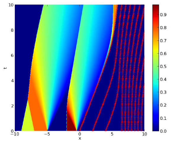
Figure 2: Numerical integration of the LWR–FtL model (2.4)–(3.1)–(3.2). The interplay between the micro- and macroscopic phases is shown by the shock arising at about $t=4$, fully visible from about $t=8$.

The resulting solution is displayed in the $(t,x)$ plane in Figure 2. It was computed with a space mesh size $\Delta x=2.5\times 10^{-3}$ and a time mesh size updated at each time step so that

$$\Delta t=0.9\cdot\Delta x/\Lambda$$ (3.3)

$\Lambda$ being the maximal characteristic speed.

On the left, we see the typical behavior of the solutions to the LWR model, consisting of shocks and rarefaction waves. On the right, the microscopic part yields the trajectories of the single vehicles. Due to the choice (3.2) of the initial datum, the cars in front start very slowly, while the ones in the back have a higher initial speed. After a while these latter vehicles have to brake, according to (1.2). This causes the formation of a shock in the macroscopic phase. Indeed, at about $t=4$, behind the leftmost driver, a shock starts forming and becomes visible at about $t=8$.

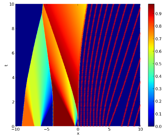
Figure 3: Numerical integration of the LWR–FtL model (2.4)–(3.1)–(3.4). Here, we used the same space and time meshes as in the integration leading to Figure 2.

The same setting (2.4)–(3.1), but with initial datum

$$\begin{array}[]{rcl}\bar{\rho}(x)&=&\mathbf{\chi}_{[-4,-0.5]}(x)+0.6\mathbf{\chi}_{[-6,-7]}(x)+0.8\mathbf{\chi}_{[-9,-7]}(x)\\ \bar{p}&=&\left[0,\,0.5,\,1.,\,1.5,\,2.,\,,\,2.5,\,3.,\,3.5,\,4.,\,4.5,\,5.,\,7.,\,8.,\,9.,\,10.\right]\end{array}$$ (3.4)

leads to the picture in Figure 3. Here, the leftmost drivers in the microscopic phase have a very low initial speed. Hence, the rightmost vehicles in the macroscopic phase have to brake at about $t=0.5$, forming a queue. Later, the drivers in the microscopic phase accelerate and this increase in the speeds reaches also the macroscopic phase.

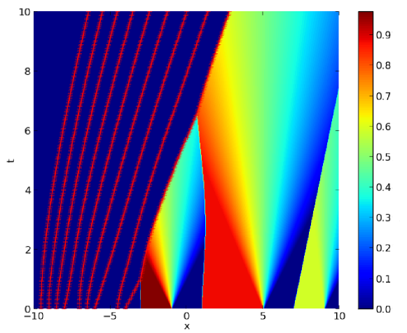
Figure 4: Numerical integration of the FtL–LWR model (2.5)–(3.1)–(3.5). The LWR density in the interval $[-3,\,-1]$ is maximal, hence the traffic speed vanishes there. As a consequence, the first vehicle in the microscopic phase reaches the phase boundary at about $t=2$ and at that time its velocity is discontinuous.

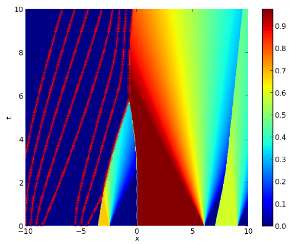
Figure 5: Numerical integration of the FtL–LWR model (2.5)–(3.1)–(3.6). Here, we used the same space and time meshes as in the integration leading to Figure 4. The first vehicle in the macroscopic phase reaches the phase boundary at about $t=1.5$ and at that time its velocity is discontinuous. In the macroscopic phase, at that time, there is an interaction between a shock and a rarefaction curve.

In the other case of the FtL-LWR model (2.5), we keep using the choices (3.1), but with the initial datum

$$\begin{array}[]{rcl}\bar{\rho}(x)&=&\mathbf{\chi}_{[-3,-1]}(x)+0.9\mathbf{\chi}_{[1,5]}(x)+0.6\mathbf{\chi}_{[7,9]}(x)\\ \bar{p}&=&\left[-9.5,-9,-8.5,-8,-7,-6.5,-6,-4.5,-4\right]\end{array}$$ (3.5)

with a mesh $\Delta x=10^{-3}$ and a time mesh chosen as in (3.3). The resulting solution is displayed in the $(t,x)$ plane in Figure 4. Differently from what usually happens in the usual FtL model, here the speed of the first vehicle suffers a discontinuity, clearly visible at about $t=1$, due to its reaching the interface with the LWR phase.

The same setting in (2.5), with the choices (3.1), but with the initial datum

$$\begin{array}[]{rcl}\bar{\rho}(x)&=&0.7\mathbf{\chi}_{[-3.5,-2.5]}(x)+\mathbf{\chi}_{[0,6]}(x)+0.6\mathbf{\chi}_{[7,9]}(x)\\ \bar{p}&=&\left[-11,-10,-9.5,-9,-8.5,-5.5,-5,-4.5\right]\end{array}$$ (3.6)

leads to the representation in Figure 5.

The initial density in the LWR phase is maximal in the interval $\left[0,6\right]$. This situation has consequences also the microscopic phase. First, the speed of the leader suffers a discontinuity, clearly visible at about $t=1.5$, due to its reaching the interface with the LWR phase. Then, the drivers behind the leader have to brake.

The figures above explain how the two micro- and macroscopic descriptions coexist in a single model. There is a clear backward propagating exchange of information between the different phases, although there is no exchange of mass.

4 Technical Details

The following Lemma deals with the ordinary differential system (1.2). Its proof reminds that of [6, Proposition 4.1].

Lemma 4.1.

Let $v$ satisfy (v) and $\ell>0$. Choose $\bar{p}\in\mathcal{P}_{\ell}^{n}$. Let $w\in\mathbf{L^{1}_{loc}}({\mathbb{R}}^{+};{\mathbb{R}}^{+})$. Then, the Cauchy problem

$$\left\{\begin{array}[]{ll}\dot{p}_{i}=v\left(\frac{\ell}{p_{i+1}-p_{i}}\right)\qquad i=1,\ldots,n-1\\ \dot{p}_{n}=w(t)\\ p_{i}(0)=\bar{p}_{i}\end{array}\right.$$ (4.1)

admits a unique solution $p=p(t)$ defined for all $t\in{\mathbb{R}}^{+}$ and attaining values in $\mathcal{P}_{\ell}^{n}$. Moreover, if $w^{\prime}\in\mathbf{L^{1}_{loc}}({\mathbb{R}}^{+};{\mathbb{R}}^{+})$, $\bar{p}^{\prime}\in\mathcal{P}_{\ell}$ and $p^{\prime}=p^{\prime}(t)$ is the corresponding solution to (4.1), the following stability estimate holds

$${\left\|p(t)-p^{\prime}(t)\right\|}\leq\left({\left\|\bar{p}-\bar{p}^{\prime}\right\|}+{\left\|w-w^{\prime}\right\|}_{\mathbf{L^{1}}([0,t])}\right)\exp{\left(2\frac{\mathbf{Lip}(v)}{\ell}t\right)},$$ (4.2)

for every $t\in\left]0,+\infty\right[$.

Proof.

By (v), the function $v$ can be extended to a bounded Lipschitz function $u$ defined on all ${\mathbb{R}}$ setting

$$u(\rho)=\left\{\begin{array}[]{l@{\qquad\mbox{ if}\qquad}r@{\,}c@{\,}l}v(0)&\rho&<&0\\ v(\rho)&\rho&\in&[0,1]\\ 0&\rho&>&1\,.\end{array}\right.$$ (4.3)

Now we consider the Cauchy problem

$$\left\{\begin{array}[]{ll}\dot{p}_{i}=u\left(\frac{\ell}{p_{i+1}-p_{i}}\right)&i=1,\ldots,n-1\\ \dot{p}_{n}=w(t)\\ p_{i}(0)=\bar{p}_{i}&i=1,\ldots,n\,.\end{array}\right.$$ (4.4)

By the standard ODE theory, there exists a $\mathbf{C^{1}}$ solution $p=p(t)$ defined as long as $p_{i+1}-p_{i}>0$ for all $i=1,\ldots,n-1$. We now prove that in fact $p_{i+1}(t)-p_{i}(t)\geq l$ for every $t\geq 0$. To this aim, we assume by contradiction that there exists $t^{*}$ in ${\mathbb{R}}^{+}$, such that $p_{i+1}(t^{*})-p_{i}(t^{*})<l$. Then, since $p_{i+1}(0)-p_{i}(0)=\bar{p}_{i+1}-\bar{p}_{i}\geq l$, there exists $\bar{t}$ in ${\mathbb{R}}^{+}$, with $\bar{t}<t^{*}$, such that $p_{i+1}(\bar{t})-p_{i}(\bar{t})=l$ and $p_{i+1}(t)-p_{i}(t)<l$ for every $t\in\left]\bar{t},t^{*}\right]$. Since $u(\rho)=0$ for every $\rho>1$, for every $t\in\left]\bar{t},t^{*}\right]$, we have

$$p_{i}(t)=p_{i}(\bar{t})+\int_{\bar{t}}^{t}\!\dot{p}_{i}(s)\,ds=p_{i}(\bar{t})+\int_{\bar{t}}^{t}u\left(\frac{\ell}{p_{i+1}(s)-p_{i}(s)}\right)ds=p_{i}(\bar{t}).$$

This yields a contradiction, since for every $t\in\left]\bar{t},t^{*}\right]$ and for $i=1,\ldots,n-1$,

$$p_{i+1}(t)-p_{i}(t)\geq p_{i+1}(\bar{t})-p_{i}(\bar{t})=l,$$

completing the existence proof.

To prove the estimate (4.2), observe that the right hand side in (4.1) is Lipschitz continuous, indeed

$${\left|v\left(\frac{\ell}{p_{i+1}-p_{i}}\right)-v\left(\frac{\ell}{p_{i+1}^{\prime}-p_{i}^{\prime}}\right)\right|}\leq\frac{\mathbf{Lip}(v)}{\ell}\left({\left|p_{i+1}-p_{i+1}^{\prime}\right|}+{\left|p_{i}-p_{i}^{\prime}\right|}\right)\,.$$ (4.5)

for $i=1,\ldots,n-1$. Hence, by (4.5),

$${\left|p_{i}(t)-p_{i}^{\prime}(t)\right|} \leq {\left|\bar{p}_{i}-\bar{p}_{i}^{\prime}\right|}+\int_{0}^{t}{\left|v\left(\frac{\ell}{p_{i+1}-p_{i}}\right)-v\left(\frac{\ell}{p_{i+1}^{\prime}-p_{i}^{\prime}}\right)\right|}\mathinner{\mathrm{d}{s}}$$ (4.6)

$$\leq {\left|\bar{p}_{i}-\bar{p}_{i}^{\prime}\right|}+\frac{\mathbf{Lip}(v)}{\ell}\int_{0}^{t}\left({\left|p_{i+1}-p_{i+1}^{\prime}\right|}+{\left|p_{i}-p_{i}^{\prime}\right|}\right)\mathinner{\mathrm{d}{s}}$$

$$\leq {\left\|\bar{p}-\bar{p}^{\prime}\right\|}+2\frac{\mathbf{Lip}(v)}{\ell}\int_{0}^{t}{\left\|p(s)-p^{\prime}(s)\right\|}\mathinner{\mathrm{d}{s}}\,,$$

On the other hand, For $i=n$, we immediately have

$${\left|p_{n}(t)-p_{n}^{\prime}(t)\right|}\leq{\left\|\bar{p}-\bar{p}^{\prime}\right\|}+{\left\|w-w^{\prime}\right\|}_{\mathbf{L^{1}}\left(\left[0,t\right]\right)}\,.$$ (4.7)

Hence, (4.6) and (4.7) together yield

$${\left\|p(t)-p^{\prime}(t)\right\|}\leq{\left\|\bar{p}-\bar{p}^{\prime}\right\|}+{\left\|w-w^{\prime}\right\|}_{\mathbf{L^{1}}\left(\left[0,t\right]\right)}+2\frac{\mathbf{Lip}(v)}{\ell}\int_{0}^{t}{\left\|p(s)-p^{\prime}(s)\right\|}\mathinner{\mathrm{d}{s}}$$

and an application of the usual Gronwall Lemma gives (4.2). ∎

Lemma 4.2.

Let $v$ satisfy (v). Fix $\gamma\in\mathbf{C^{0,1}}({\mathbb{R}}^{+}{\mathbb{R}})$, $\bar{\rho}\in(\mathbf{L^{1}}\cap\mathbf{BV})({\mathbb{R}};[0,1])$ and $\tilde{\rho}\in(\mathbf{L^{1}}\cap\mathbf{BV})({\mathbb{R}}^{+};[0,1])$. Then, the initial – boundary value problem

$$\left\{\begin{array}[]{l@{\qquad}rcl}\partial_{t}\rho+\partial_{x}\left(\rho\,v(\rho)\right)=0&x&<&\gamma(t)\\ \rho(0,x)=\bar{\rho}(x)&x&<&\gamma(0)\\ \rho\left(t,\gamma(t)\right)=\tilde{\rho}(t)&t&\geq&0\end{array}\right.$$ (4.8)

admits a unique weak entropy solution $\rho\in\mathbf{C^{0,1}}({\mathbb{R}}^{+};(\mathbf{L^{1}}\cap\mathbf{BV})\left({\mathbb{R}};[0,1])\right)$.

Moreover, there exists a constant $L>0$ such that if $\gamma,\gamma^{\prime}\in\mathbf{C^{0,1}}({\mathbb{R}}^{+}{\mathbb{R}})$ with $\mathbf{Lip}(\gamma),\mathbf{Lip}(\gamma^{\prime})\leq V$ for a $V>0$, $\bar{\rho},\bar{\rho}^{\prime}\in(\mathbf{L^{1}}\cap\mathbf{BV})({\mathbb{R}};[0,1])$ and $\tilde{\rho},\tilde{\rho}^{\prime}\in(\mathbf{L^{1}}\cap\mathbf{BV})({\mathbb{R}}^{+};[0,1])$, then, the two solutions $\rho=\rho(t,x)$ and $\rho^{\prime}=\rho^{\prime}(t,x)$ to (4.8) satisfy for all $t\in{\mathbb{R}}^{+}$

$${\left\|\rho(t)-\rho^{\prime}(t)\right\|}_{\mathbf{L^{1}}}\leq L\left({\left\|\bar{\rho}-\bar{\rho}^{\prime}\right\|}_{\mathbf{L^{1}}}+{\left\|\gamma-\gamma^{\prime}\right\|}_{\mathbf{C^{0}}\left(\left[0,t\right]\right)}+(1+2V){\left\|\tilde{\rho}-\tilde{\rho}^{\prime}\right\|}_{\mathbf{L^{1}}\left(\left[0,t\right]\right)}\right).$$ (4.9)

The initial – boundary value problem in (4.8) falls within the framework of [5], see also [8, 11]. Indeed, the scalar conservation law (1.1) is a particular case of a Temple systems, see [5, (H1), (H2) and (H3)]. Hence, [5, Theorem 2.3] applies and Lemma 4.2 follows.

Proof of Proposition 2.2.  In (2.4), the equations for $p_{1},\ldots,p_{n}$ are decoupled from the partial differential equation for $\rho$. Hence, Lemma 4.1 applies and ensures the existence of $p=p(t)$, with $p(t)\in\mathcal{P}_{\ell}^{n}$, solving the ordinary differential system for all $t\in{\mathbb{R}}^{+}$. We then choose $\rho$ as the solution to the initial – boundary value problem

$$\left\{\begin{array}[]{l@{\qquad}rcl}\partial_{t}\rho+\partial_{x}\left(\rho\,v(\rho)\right)=0&(t,x)&\in&\left\{(t,x)\in{\mathbb{R}}^{+}\times{\mathbb{R}}\colon x<p_{1}(t)\right\}\\ \rho(0,x)=\bar{\rho}(x)&x&<&\bar{p}_{1}\\ \rho\left(t,p_{1}(t)\right)=\frac{\ell}{p_{2}(t)-p_{1}(t)}&t&\in&{\mathbb{R}}^{+}\end{array}\right.$$ (4.10)

and we apply Lemma 4.2, obtaining the existence of a map $\rho\in\mathbf{C^{0}}\left([0,T];(\mathbf{L^{1}}\cap\mathbf{BV})({\mathbb{R}};[0,1])\right)$ solving (4.10) in the usual sense of [8, Definition 2.1], [1, Definition C.1] or, equivalently, [5, Definition 2.2]. Therefore, 1. and 2 in Definition 2.1 hold, The requirements 3. and 4. follow from Lemma 4.1.

The stability estimate related to the ordinary differential system follows from Lemma 4.1. Concerning the partial differential equation, by (4.9) we have

$${\left\|\rho(t,\cdot)-\rho^{\prime}(t,\cdot)\right\|}_{\mathbf{L^{1}}} \leq L\left({\left\|\bar{\rho}-\bar{\rho}^{\prime}\right\|}_{\mathbf{L^{1}}}+{\left\|p_{1}-p_{1}^{\prime}\right\|}_{\mathbf{C^{0}}\left(\left[0,t\right]\right)}\right)$$ (4.11)

$$+L(1+2V){\left\|\frac{\ell}{p_{2}(\cdot)-p_{1}(\cdot)}-\frac{\ell}{p_{2}^{\prime}(\cdot)-p_{1}^{\prime}(\cdot)}\right\|}_{\mathbf{L^{1}}\left([0,t]\right)}.$$

Compute the term in parentheses separately

$${\left\|\frac{\ell}{p_{2}(\cdot)-p_{1}(\cdot)}-\frac{\ell}{p_{2}^{\prime}(\cdot)-p_{1}^{\prime}(\cdot)}\right\|}_{\mathbf{L^{1}}([0,t])} \leq \frac{1}{\ell}\int_{0}^{t}\left({\left|p_{2}-p_{2}^{\prime}\right|}+{\left|p_{1}-p_{1}^{\prime}\right|}\right)\mathinner{\mathrm{d}{s}}$$

$$\leq \frac{2}{\ell}\int_{0}^{t}{{\left\|p(s)-p^{\prime}(s)\right\|}ds}$$

$$\leq \frac{2}{\ell}\,t\,{\left\|p-p^{\prime}\right\|}_{\mathbf{C^{0}}\left(\left[0,t\right]\right)}$$

and inserting the above result in (4.11), using (4.2), we obtain:

$${\left\|\rho(t,\cdot)-\rho^{\prime}(t^{\prime},\cdot)\right\|}_{\mathbf{L^{1}}}$$

$$\leq L{\left\|\bar{\rho}-\bar{\rho}^{\prime}\right\|}_{\mathbf{L^{1}}}+L{\left\|p_{1}-p_{1}^{\prime}\right\|}_{\mathbf{C^{0}}\left(\left[0,t\right]\right)}+L\left(1+2V\right)\frac{2}{\ell}t{\left\|p-p^{\prime}\right\|}_{\mathbf{C^{0}}([0,t])}$$

$$\leq L{\left\|\bar{\rho}-\bar{\rho}^{\prime}\right\|}_{\mathbf{L^{1}}}+L\left(1+(1+2V)\frac{2}{\ell}\,t\right){\left\|p-p^{\prime}\right\|}_{\mathbf{C^{0}}([0,t])}$$

$$\leq L{\left\|\bar{\rho}-\bar{\rho}^{\prime}\right\|}_{\mathbf{L^{1}}}+L\left(1+(1+2V)\frac{2}{\ell}\,t\right)\left({\left\|\bar{p}-\bar{p}^{\prime}\right\|}+{\left\|w-w^{\prime}\right\|}_{\mathbf{L^{1}}([0,t])}\right)\exp\left(2\frac{\mathbf{Lip}(v)}{\ell}t\right)$$

completing the proof.   $\square$

Proof of Proposition 2.3.  To construct a solution to (2.5), we first apply [4, Theorem 6.3] to obtain a Kružkov solution $\rho=\rho(t,x)$ to the Cauchy problem for the scalar conservation law

$$\left\{\begin{array}[]{l@{\qquad}rcl}\partial_{t}\rho+\partial_{x}\left(\rho\,v(\rho)\right)=0&(t,x)&\in&{\mathbb{R}}^{+}\times{\mathbb{R}}\\ \rho(0,x)=\left\{\begin{array}[]{l@{\qquad\mbox{ if}\qquad}r@{\,}c@{\,}l}\bar{\rho}(x)&x&>&\bar{p}_{n}\\ 0&x&<&\bar{p}_{n}\,.\end{array}\right.\end{array}\right.$$ (4.12)

Then, we find the free boundary $p_{n}=p_{n}(t)$ solving the Cauchy problem for the ordinary differential equation

$$\left\{\begin{array}[]{l}\dot{p}_{n}=v\left(\rho\left(t,p_{n}(t)\right)\right)\\ p_{n}(0)=\bar{p}_{n}\,.\end{array}\right.$$ (4.13)

The well posedness of (4.13) is ensured by [7, Theorem 2.4], which we can apply due to (v), see also [7, Item 1 in Section 2].

Next we restrict the solution $\rho=\rho(t,x)$ to (4.12) to $\left\{(t,x)\in{\mathbb{R}}^{+}\times{\mathbb{R}}:x>p_{n}(t)\right\}$. Then, we solve the following system of $n-1$ ordinary differential equations

$$\left\{\begin{array}[]{l}\dot{p}_{i}=v\left(\frac{\ell}{p_{i+1}-p_{i}}\right)\qquad i=1,\ldots,n-1\\ p_{i}(0)=\bar{p}_{i}\,.\end{array}\right.$$ (4.14)

By construction, 1. in Definition 2.1 holds. Condition 2. is in this case empty. The requirement 4. is satisfied since $p_{n}$ solves (4.13) and the previous application of Lemma 4.1 to (4.14) ensures 3.

Passing to the stability estimates, using [4, (ii) in Theorem 6.3], we have

$${\left\|\rho(t)-\rho^{\prime}(t)\right\|}_{\mathbf{L^{1}}} \leq \int_{{\mathbb{R}}}{\left|\bar{\rho}(x)\,\mathbf{\chi}_{[\bar{p}_{n}^{\prime},+\infty[}(x)-\bar{\rho}^{\prime}(x)\,\mathbf{\chi}_{[\bar{p}_{n}^{\prime},+\infty[}(x)\right|}\mathinner{\mathrm{d}{x}}$$

$$\leq {\left\|\bar{\rho}-\bar{\rho}^{\prime}\right\|}_{\mathbf{L^{1}}}+{\left|\bar{p}_{n}-\bar{p}_{n}^{\prime}\right|}$$

$$\leq {\left\|\bar{\rho}-\bar{\rho}^{\prime}\right\|}_{\mathbf{L^{1}}}+{\left\|\bar{p}-\bar{p}^{\prime}\right\|}\,,$$

proving (2.6). to prove (2.7), we use [7, Theorem 2.2] to obtain, in the case $\bar{\rho}=\bar{\rho}^{\prime}$,

$${\left|p_{n}(t)-p_{n}^{\prime}(t)\right|}\leq c(t)\,{\left|\bar{p}-\bar{p}^{\prime}\right|}^{\alpha}$$

where $c$ is the constant exhibited in [7, Item (2), Theorem 2.2] with respect to the interval $[0,t]$ and , by [7, formula (2.1)],

$$1-\alpha\geq\max_{\rho\in[0,R]}\frac{v(\rho)-v(0)}{v(0)-v(\rho)-\rho\,v^{\prime}(\rho)}\quad\mbox{or, equivalently}\quad\alpha=\left(1+\max_{[0,R]}\frac{v(\rho)-v(0)}{\rho\,v^{\prime}(\rho)}\right)^{-1}$$

which is finite by (v). Finally, (2.7) directly follows from Lemma 4.1.   $\square$

Proof of Proposition 2.4.  Use the integral form of the conservation law (1.1) in the region

$$\Omega=\left\{(\tau,\xi)\in{\mathbb{R}}^{+}\times{\mathbb{R}}\colon\tau\in[0,t]\mbox{ and }\xi\in[p_{n_{j}}^{j}(t),p_{1}^{j+1}(t)]\right\}$$

and obtain:

$$\int_{p_{n_{j}}^{j}(t)}^{p_{1}^{n_{j+1}}(t)}\rho(t,x)\mathinner{\mathrm{d}{x}}\!\!\! - \!\!\!\int_{\bar{p}_{n_{j}}^{j}}^{\bar{p}_{1}^{j+1}}\bar{\rho}(x)\mathinner{\mathrm{d}{x}}=$$

$$= \int_{0}^{t}\left[\rho\left(\tau,p_{n_{j}}^{j}(\tau)\right)\quad(\rho\,v)\left(\tau,p_{n_{j}}^{j}(\tau)\right)\right]\left[\begin{array}[]{c}-\dot{p}_{n_{j}}^{j}(\tau)\\ 1\end{array}\right]\mathinner{\mathrm{d}{\tau}}$$

$$+\int_{0}^{t}\left[\rho\left(\tau,p_{1}^{j+1}(\tau)\right)\quad(\rho\,v)\left(\tau,p_{1}^{j+1}(\tau)\right)\right]\left[\begin{array}[]{c}\dot{p}_{1}^{j+1}(\tau)\\ -1\end{array}\right]\mathinner{\mathrm{d}{\tau}}$$

$$= \int_{0}^{t}\left[\rho\left(\tau,p_{n_{j}}^{j}(\tau)\right)\quad(\rho\,v)\left(\tau,p_{n_{j}}^{j}(\tau)\right)\right]\left[\begin{array}[]{c}-v\left(\tau,p_{n_{j}}^{j}(\tau)\right)\\ 1\end{array}\right]\mathinner{\mathrm{d}{\tau}}$$

$$+\int_{0}^{t}\frac{\ell}{p_{2}^{j+1}(\tau)-p_{1}^{j+1}(\tau)}\left[1\quad v\left(\frac{\ell}{p_{2}^{j+1}(\tau)-p_{1}^{j+1}(\tau)}\right)\right]\left[\begin{array}[]{c}\dot{p}_{1}^{j+1}(\tau)\\ -1\end{array}\right]\mathinner{\mathrm{d}{\tau}}$$

$$= 0$$

since $(p,\rho)$ solves (2.2) in the sense of Definition 2.1.   $\square$

References

• [1] D. Amadori and R. M. Colombo. Viscosity solutions and standard Riemann semigroup for conservation laws with boundary. Rend. Sem. Mat. Univ. Padova, 99:219–245, 1998.
• [2] B. Argall, E. Cheleshkin, J. M. Greenberg, C. Hinde, and P.-J. Lin. A rigorous treatment of a follow-the-leader traffic model with traffic lights present. SIAM J. Appl. Math., 63(1):149–168 (electronic), 2002.
• [3] A. Aw and M. Rascle. Resurrection of “second order” models of traffic flow. SIAM J. Appl. Math., 60(3):916–938 (electronic), 2000.
• [4] A. Bressan. Hyperbolic systems of conservation laws, volume 20 of Oxford Lecture Series in Mathematics and its Applications. Oxford University Press, Oxford, 2000. The one-dimensional Cauchy problem.
• [5] R. M. Colombo and A. Groli. On the initial boundary value problem for Temple systems. Nonlinear Anal., 56(4):569–589, 2004.
• [6] R. M. Colombo, F. Marcellini, and M. Rascle. A 2-phase traffic model based on a speed bound. SIAM J. Appl. Math., 70(7):2652–2666, 2010.
• [7] R. M. Colombo and A. Marson. A Hölder continuous ODE related to traffic flow. Proc. Roy. Soc. Edinburgh Sect. A, 133(4):759–772, 2003.
• [8] F. Dubois and P. Lefloch. Boundary conditions for nonlinear hyperbolic systems of conservation laws. J. Differential Equations, 71(1):93–122, 1988.
• [9] M. Garavello and B. Piccoli. On fluido-dynamic models for urban traffic. Netw. Heterog. Media, 4(1):107–126, 2009.
• [10] C. Lattanzio and B. Piccoli. Coupling of microscopic and macroscopic traffic models at boundaries. Math. Models Methods Appl. Sci., 20(12):2349–2370, 2010.
• [11] P. G. Lefloch. Explicit formula for scalar nonlinear conservation laws with boundary condition. Math. Methods Appl. Sci., 10(3):265–287, 1988.
• [12] R. J. LeVeque. Numerical methods for conservation laws. Lectures in Mathematics ETH Zürich. Birkhäuser Verlag, Basel, second edition, 1992.
• [13] M. J. Lighthill and G. B. Whitham. On kinematic waves. II. A theory of traffic flow on long crowded roads. Proc. Roy. Soc. London. Ser. A., 229:317–345, 1955.
• [14] P. I. Richards. Shock waves on the highway. Operations Res., 4:42–51, 1956.
• [15] H. Zhang. A non-equilibrium traffic model devoid of gas-like behavior. Transportation Research Part B: Methodological, 36(3):275 – 290, 2002.